Article

A Novel Framework for Portfolio Selection Model Using Modified ANFIS and Fuzzy Sets

by
Chanchal Kumar
* and
Mohammad Najmud Doja
Department of Computer Engineering, Jamia Millia Islamia, New Delhi 110025, India
*
Author to whom correspondence should be addressed.
Computers 2018, 7(4), 57; https://doi.org/10.3390/computers7040057
Submission received: 21 September 2018 / Revised: 17 October 2018 / Accepted: 26 October 2018 / Published: 31 October 2018

Abstract

:
This paper proposes a novel framework for solving the portfolio selection problem. This framework is excogitated using two newly parameters obtained from an existing basic mean variance model. The scheme can prove entirely advantageous for decision-making while using computed values of these significant parameters. The framework combines effectiveness of the mean-variance model and another significant parameter called Conditional-Value-at-Risk (CVaR). It focuses on extracting two newly parameters viz. αnew and βnew, which are demarcated from results obtained from mean-variance model and the value of CVaR. The method intends to minimize the overall cost, which is computed in the framework using quadratic equations involving these newly parameters. The new structure of ANFIS is designed by changing existing structure of ANFIS and this new structure contains six layers instead of existing five-layered structure. Fuzzy sets are harnessed for the design of the second layer of this new ANFIS structure. The output parameter acquired from the sixth layer of the new ANFIS structure serves as an important index for an investor in the decision-making. The numerical results acquired from the framework and the new six-layered structure is presented and these results are assimilated and compared with the results of the existing ANFIS structure.

1. Introduction

The core pursuit in the portfolio selection issue is to seek for an optimal solution that can be used by an investor for making a decision on investing a stipulated amount, provided that a set of assets or securities is disposed. Primarily, a portfolio may be defined in terms of finding a solution among the numerous ways for distributing this invested amount between different assets. A prevalent model named a mean-variance model for finding an appropriate solution of the above-mentioned portfolio selection case has been presented by Markowitz [1]. The overall return of a portfolio is characterized in terms of mean value of the gain of the investments and risk amidst different investments [1]. An eligible optimization solution can be characterized in terms of portfolios, which seek the minimal risk for a disposed of the value of return. Moreover, for a disposed of the mean value of return, an eligible optimization solution confers the excellent optimal way of investing this amount. Nevertheless, a constraint, which will ensure an optimal investment made for a variety of assets, is lacking in the above-mentioned model. A description of another constraint that is capable of binding the limit for the investing amount is also not defined in the above-mentioned model. These constraints play a significant role for an investor; therefore, to overcome these deficiencies, the constraints must be included in the changed framework. An effective way of contriving a new framework is put forward in this paper, so that an efficient solution for this optimization problem may be found that will have an optimal solution, considering the efficacy of the above-mentioned mean-variance model and another significant parameter viz. Conditional-Value-at-Risk (CVaR). The structure of the new framework is demarcated using two newly parameters which are derived from the results obtained from basic mean-variance model and CVaR. The objective of this framework is to minimize the overall cost that is being computed using quadratic equations based on these newly parameters.

1.1. Related Work

Heuristic methods have been employed for the solution of portfolio optimization problem and the majority of researchers have exploited evolutionary algorithms concept for the above-mentioned purpose. Some researchers [2] have used the concept of constraints trustworthiness based on the event for portfolio selection. Real world investments involve multi-criteria decisions, so keeping in mind this fact some researchers [3], have developed a novel multi-objective scheme for portfolio selection based on the concept of reliability where constraints are represented by fuzzy logic. One of the major aspects of portfolio selection problem is that assets returned can be easily realized in terms of fuzzy variables. Keeping in view the above aspect researchers [4] have used the concept of reliability theory, which is formulated using fuzzy logic and the mean-variance model. The above work was further extended based on semi-variance [5] and skewness [6]. There were certain limitations of possibility measures used for portfolio selection in order to overcome the problem risk factor was included. The inclusion of risk in the portfolio selection model using fuzzy logic is given in [7]. A cross breed algorithm based on wise learning for common situations is provided. Using the concept of predicated value in a multiobjective environment based on fuzzy logic is given in [8,9]. A portfolio selection model based on fuzzy-value-at-risk is given in [10] and developed a particle swarm optimization algorithm to find the best solution. An alternative risk measure is given in [11,12], named as Conditional-Value-at-Risk (also known as Expected Shortfall, Expected Tail Loss). CVaR is thoroughly identical to VaR measure of risk for normal distributions and has better attributes than VaR. A multi-period mean-semivariance model is given in [13,14,15] for portfolio selection problem. A significant role of adaptive neuro-fuzzy inference system to stock market prediction is presented in [16,17,18,19]. Type-2 fuzzy sets play a vital role in portfolio selection, which is shown in [20,21]. A metaheuristic solution to complicated futures portfolio optimization problem is presented in [22]. Fuzzy theory based models are given in [23,24,25] to portfolio selection problem. A optimization method based on particle swarm optimization is given in [26], has applied to portfolio selection. Wang et al. [27] proposed a novel model for multiple objectives using fuzzy logic for solving a portfolio selection problem with alternative risk measure and the existing particle swarm optimization is also modified in the model. A multiple stage adaptive optimization model to portfolio optimization problem is introduced in [28]. A predication based mean-variance model to solve the constrained portfolio optimization is given in [29]. A description of methods employing different evolutionary algorithms in [30,31,32,33,34,35]. Some recent new version of the ANFIS are presented in [36,37,38,39]. An approach is proposed in [40,41] against the mean-variance method for portfolio selection problem named as full-scale optimisation. Allowing distributional asymmetries makes it possible to enhance mean-variance portfolio selection [42]. The optimized portfolios are better than weighted portfolio [43]. For the in copula opinion pooling (COP) technique for getting the returns of assets from modelling co-dependence, it has been recommended to use multivariate t-copula. However, for describing the dependence structure in high-dimensional cases, t-copula is not as flexible as vine copula [44]. Problems pertaining to portfolio selection can be optimized with a utility optimization approach known as Full-Scale Optimization (FSO), which is theoretically appealing, but, when it comes to massive scale problems, it gets burdened with computations. Hence, in order to overcome this problem, one heuristic algorithm named as differential evolution is applied in [45]. A comparative study of distance, co-integration, and copula Methods is presented in [46] regarding the pairs trading. A comparative study of mean-variance model and full-scale optimization model is given in [47].

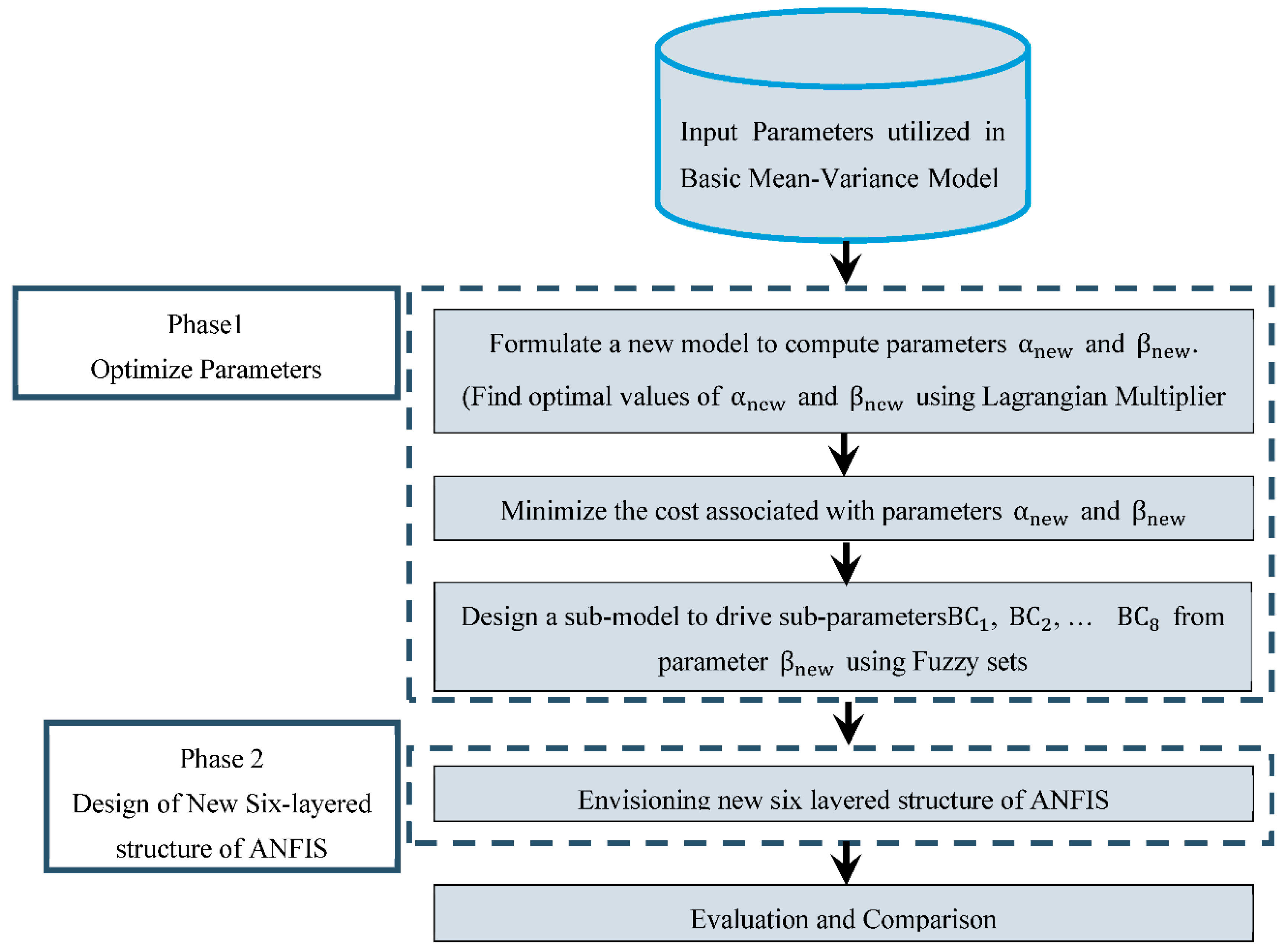
1.2. Concept of the Proposed Framework

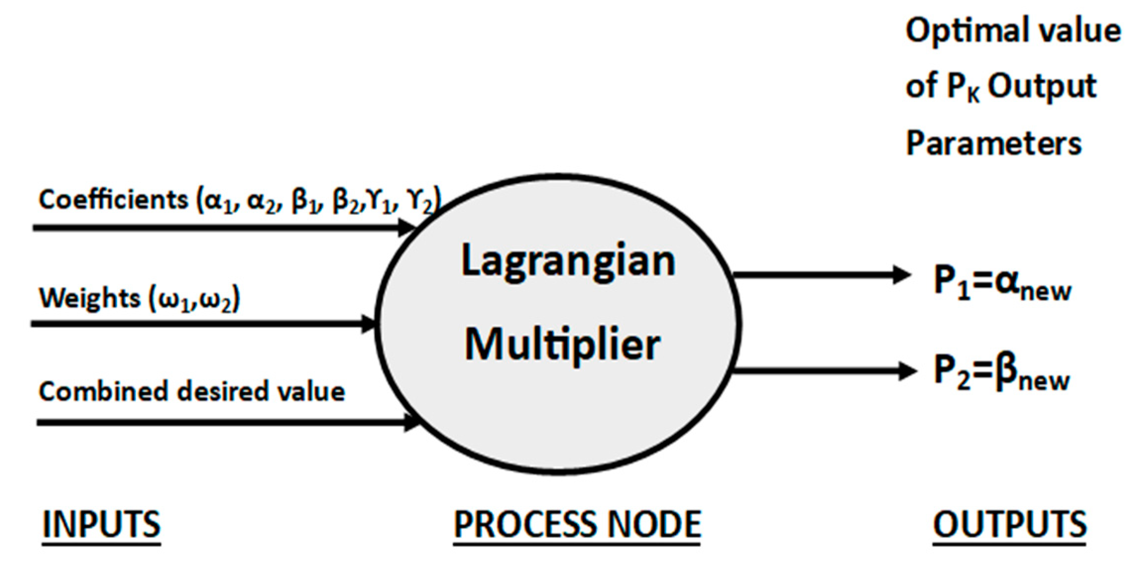
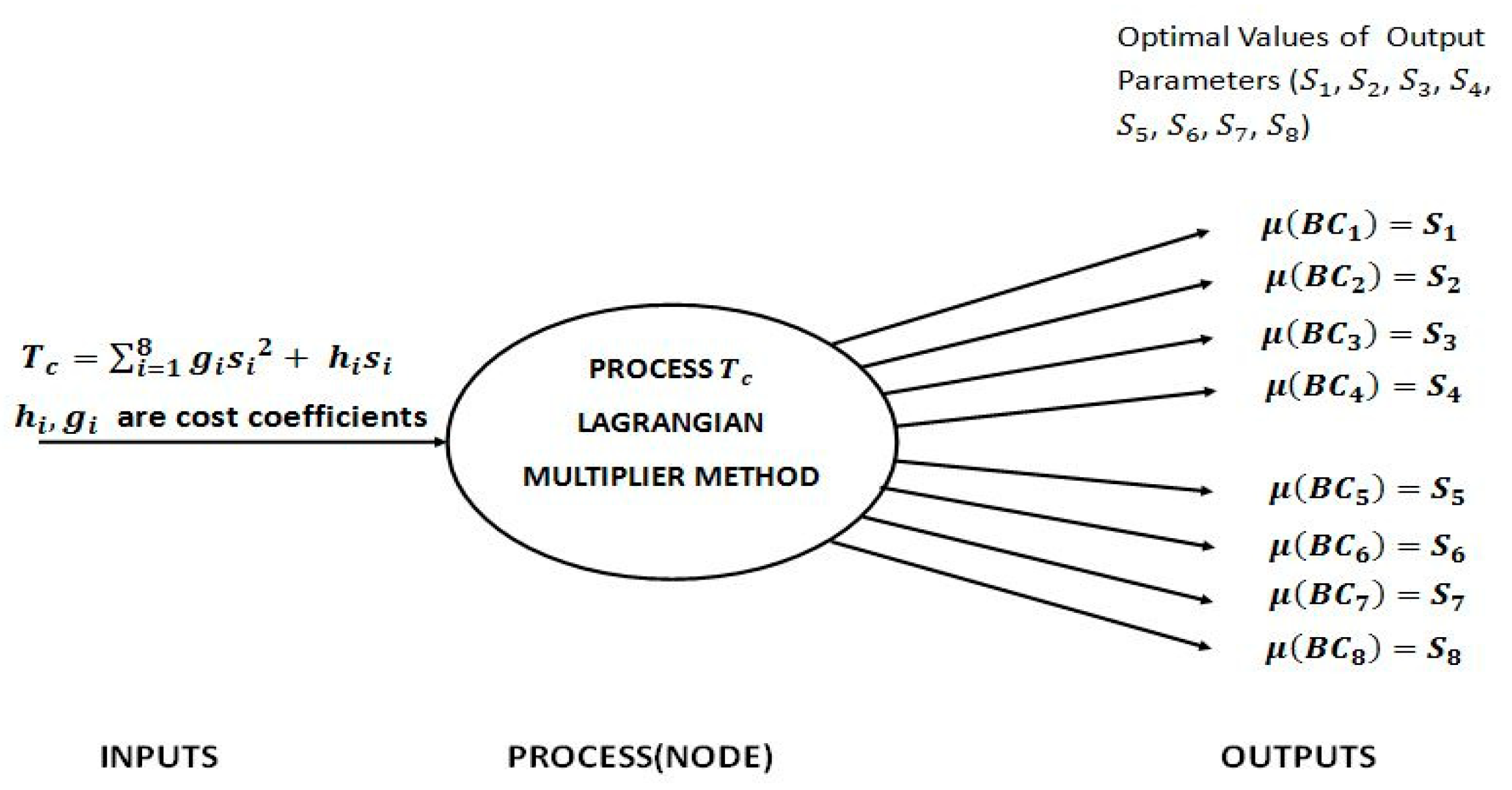
1.2.1. Phase 1. Optimization of Newly Derived Parameters

Formulating a framework of the issue of portfolio selection is completed by minimizing the costs, which are calculated from two newly parameters viz. α new and β new . The first parameter α new is computed from the output values obtained from the basic mean-variance model. The cost calculated from parameter α new is given by quadratic Equation (4). Drafting the value of the parameter β new is made by correlating another significant value, which is Conditional-Value-at-Risk. Thus, the parameter β new has a significant contribution in the framework for depicting variation in the portfolio selection model. The cost calculated from the parameter β new is given by quadratic Equation (5). The computation of the optimal values of the costs is made by using a classical Lagrangian multiplier method. The description of the parameters used in the proposed framework is given below:
Objective function Minimized value of { C 1 + C 2 },
α new First parameter used in the proposed framework whose value is derived from the output values obtained from the basic mean-variance model,
β new The second derived parameter whose value is derived from another important parameter Conditional-Value-at-Risk,
C 1 Cost computed from parameter α new ,
C 2 Cost computed from parameter β new .
This proposed framework has a description of a novel scheme, which is used for computing the values of the parameters α new and β new . The classical Lagrangian multiplier method is used in the proposed framework for finding the optimal values of the costs C 1 and C 2 . Furthermore, a scheme is formulated for generating a model which computes eight new sub-parameters viz. BC 1 , BC 2 , , BC 8 from the computed value of the parameter β new . These sub parameters are essential in the decision-making process related to bounding values of the parameter β new . Therefore, these values can be utilized by a decision maker of portfolio selection, in selecting an appropriate value of the parameter β new . The value of the parameter β new is correlated with Conditional-Value-at-Risk; therefore, it plays a significant role in the decision-making. The amount of risk and the level uncertainty can be controlled by selecting an appropriate value of the parameter β new in the proposed framework. Fuzzy sets are used in the proposed framework for framing the values of the sub parameters. The fuzzy sets are employed so that uncertainty can be included in the proposed framework. Without the inclusion of appropriate level of uncertainty, the accurate modeling of risk in the model can not be achieved. Hence, these sub-parameters, which are described in this paper, has contributed significantly towards accurately depicting risk in the portfolio selection.

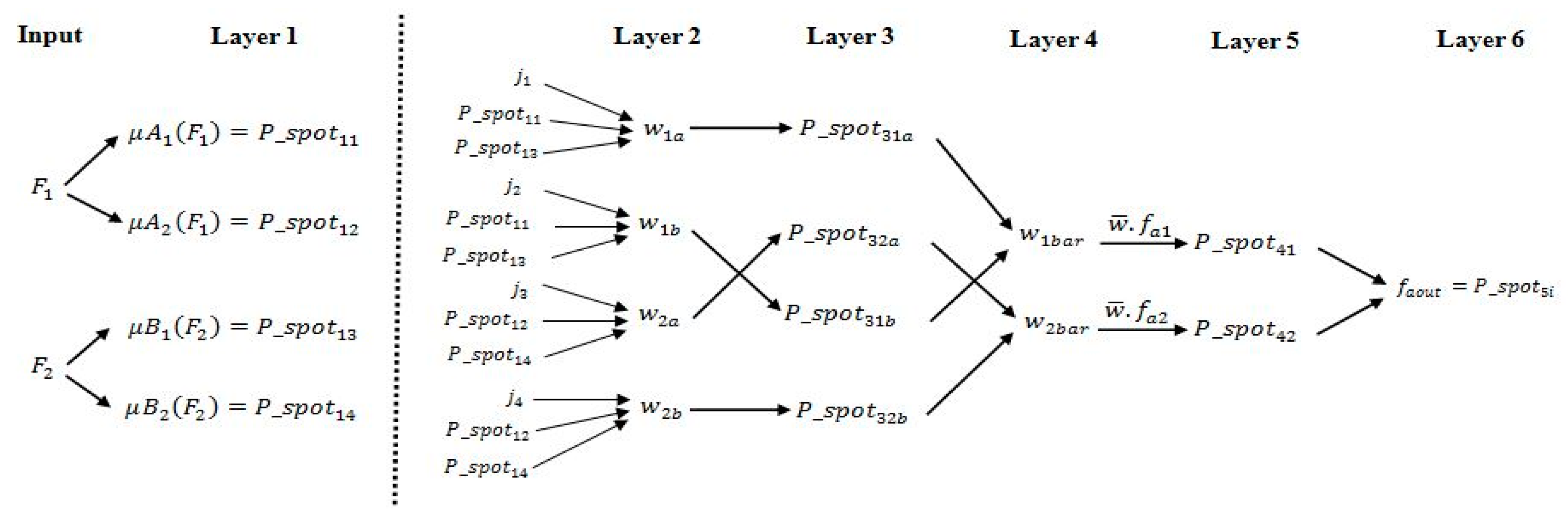
1.2.2. Phase 2. Design of New Six-Layered Structure of ANFIS

As described in Phase 1, a novel scheme for bounding the value of parameter β new using sub-parameters BC 1 , BC 2 , , BC 8 is provided in proposed framework. Furthermore, to depict the role of uncertainty in financial data, a new six-layered structure of ANFIS is formulated. The newly framed structure of ANFIS may be utilized to evaluate the performance of the proposed framework. The output parameter obtained from this structure of ANFIS is a kind of benchmark for the performance of the proposed framework. The basic model of ANFIS is described in [17] and the recent new version of the ANFIS is given in [36,37,38,39]. A modified model is presented in this paper that has a new structure having six layers. Fuzzy sets are being employed for changing the structure of existing second layer (layer 2). In addition, the two rules which are used for computing parameters in fifth layer (layer 5) are optimized using the Cuckoo Intelligence Algorithm. The values of the parameters, which are used in the two rules, are selected from the output obtained from Cuckoo Intelligence Algorithm and the output obtained from this newly structured ANFIS is given in this paper.
The structure of the modified ANIS has six-layered instead of five-layered ANFIS structure. The first–layer nodes are kept the same in the modified ANFIS as well as in the existing ANFIS structure. The modified ANFIS structure uses a new parameter j i , which is employed for assigning weights nodes in second layer.
The modifications in the fifth layer of modified ANFIS is based upon optimizing parameters that are used in two rules that calculate values of nodes in this layer. Quadratic equations are used for calculating these values of optimizing parameters. Along with these optimizing parameters, the third parameter is introduced in the rules. The cuckoo intelligence algorithm is used for calculating these optimal parameters. The structure of different nodes used in the existing ANFIS and modified ANFIS is given in Table 1.

1.2.3. Economic and Statistical Significance of Using the ANFIS Structure

The significance of using ANFIS structure is given below:
  • Statistical Significance: ANFIS structure is utilized for providing a prediction capability in portfolio selection. Since forecast of expected returns may be a desirable feature in view of the investor’s selections. This prediction scheme should be capable of accurately modeling the desired parameters based on existing data points. This can be achieved by means of an ANFIS structure that has a fuzzy inference system. Furthermore, situations where ANFIS with different data points are desirable for selective time duration, an adaptive structure needs to be employed. This adaptive nature is required for a different set of parameters.
Moreover, techniques based on algorithms using artificial intelligence would be highly complex with a large set of rules. Other available techniques might require details of the types of the parameters used for prediction. These parameters would yield to complex equations, which are hard to realize. Hence, utilizing an ANFIS structure is the more practical aspect for modelling and implementation. An efficient method requiring few computations can be easily framed using this ANFIS structure.
  • Economic Significance: Designing of efficient models for portfolio selection can be suitably crafted using the computational index represented by the output of the last node in the ANFIS structure. While obtaining the expected returns in case of multi-assets data, this index can be employed as a decision parameter. The expected returns would correspondingly alter in the view of the selected value of this index. Even though a nominal value of this index is employed while designing, this scheme could substantially alter the values of expected returns. These designs may also be employed for finding an optimal solution in the areas beyond financial applications. The investor would like to select an option that yields lower values of risk.
The scheme based on ANFIS is an appropriate choice for investors, finance companies and corporates that computes risk-based solutions. It can prove useful in the case of multi-asset domains. This usage might provide solutions that depict returns based on simple implementations. In situations where risk is computed by different simulations and investor selects one of the obtained solutions, the design based on ANFIS structure may provide an accurate modelling of risk. This ANFIS structure can be combined with efficient algorithms to provide a rich variety of optimal solutions to investors. An attractive mathematical representation of computation of expected returns can be generated for usage of the investors. The different set of solutions generating by utilizing ANFIS structure will provide a chance for the investor to select an appropriate portfolio based on minimum value of the risk. The most appropriate portfolio selection may be done by the investor, who is intended to make a selective choice of the expected returns. The investor may be interested in selecting solutions that are approximate to the desired solution. Another significant aspect could be having a scheme that has capabilities to modify multiple assets together. These computations can be projected with simple representations to the investor. The structure of the proposed model is illustrated in Figure 1.

1.2.4. Advantageous of Using the Proposed Methodology

The advantage of the methodology adopted in the paper is a more accurate design of computer algorithms by including the effects of uncertain nature of data in the application. Since the randomness of input data needs to be accounted for in the desired solution, a more practical approach has to be implemented for generating an optimal solution. In general, simple gradient search algorithms are prone to slow convergence if the data values are largely varying in nature. These methods rely on computation of the gradient. A suitable algorithm needs to be selected. If the constraints are added, this might yield complex calculations. Computational difficulties may arise if any of the constraints are violated. The quadratic programming approaches may be computationally highly demanding for bigger system. The portfolio selection problem requires frequent recalculation of different application parameters, with only selected computer memory size.
Thus, the methodology applied should be simple in structure and fast at calculation. The inherent advantage of the robust methodology employed is simplicity with rich different computing parameters evaluated and different constraints may be evaluated. An additional major benefit realized by this rigorous methodology is that the optimal solution may be obtained with few computations. These applications require a similar rigorous methodology that is needed for computing various parameters associated with evaluation of the selected solution.
The remaining sections of the paper are arranged as follows. An overview of basic mean-variance model is given in Section 2 and Section 3 describes the formation of a new model for portfolio selection based on two newly derived parameters α new and β new . Section 4 has a description of sub-parameters that are generated from parameter β new . The need for the design of a model using fuzzy logic and an overview of new modified ANFIS is presented in Section 5 and Section 6. A discussion on experiment and comparison is provided in Section 7 and the conclusions is given in Section 8.

2. Overview of the Basic Mean-Variance Model

An evaluation model was proposed by Markowitz to deal with issues of portfolio optimization, which was basically a framework to analyze the nature of investment under uncertainty [1]. Returns obtained from the investment are modeled as stochastic variables and the past data is used to calculate expected values. Similarly, returns obtained from the overall portfolio are analyzed and its variance is calculated to measure risk. The Risk is also analyzed by making a comparative analysis of the returns obtained from individual assets. Joint return distribution is used to calculate a covariance matrix. Thus, a financial portfolio aims to achieve two objectives: minimizing the variance of portfolio return and maximizing the return obtained from the expected portfolio. The aim of this framework was to obtain maximum expected return with the minimum value of adversity [3]:
Min   i = 1 n j = 1 n σ ij x i x j ,
Subject to   i = 1 n r i x i = r 0 ,
i = 1 n x i = 1 ,   x i 0 ,   i = 1 , 2 , , n .
Here, r 0 represents desired return. Equation (3) describes a capital budget constraint on the proportions of the assets and Equation (4) makes sure that there is no short selling of assets. σ ij is the covariance of the returns of assets i and j, and x i is the weight of asset i in the portfolio. A sample output of the mean-variance model is given in Table 2.
The values of portfolio weights are zero for columns 1, 2, 3, 4, 6, 7 and column 9. The portfolio return is computed on a sample data given in [33]. The variations of output values of r 0 and risk are shown in Figure 2.
The different parameters and variables used in formulating the mathematical model are described below:
Combined_desired_valueDesired value of α new , β new (Input).
( weight of objective ) 1 Parameters used while correlating β new with CVaR.
( weight of objective ) 2 Parameters used while correlating β new with CVaR.
w 1 a , w 1 b , w 2 a , w 2 b Nodes of Layer 2 (Modified ANFIS).
P_spot 3 ia , P_spot 3 ib Nodes of Layer 3 (Modified ANFIS).
P_spot 4 i , P_spot 5 i Nodes of Layer 5 (Modified ANFIS).
sum 41 , sum 42 Parameters used while correlating β new with CVaR.
W k Weight associated with α new and β new .
P k The values of parameter of α new or β new .
C k Cost associated with α new or β new .
P L This term is representing loss incurred in the investment process.
w 1 , w 2 Weight associated with α new and β new respectively.
Term 7 This is a control parameter that represents maximal weighted cost associated with ( w 1 α new + w 2 β new ) .
risk max Maximum value of risk.
risk min Minimum value of risk.
SF 1 , SF 2 Scaling parameters.
α i , β i , γ i Cost coefficient used in calculating cost, c i .
sum 4 , sum 5 , sum 7 Parameters used while correlating β new with CVaR.
L Lagrangian Function.
BC i Sub parameters generated from β new using fuzzy sets.
S i Membership values from fuzzy sets associated with sub parameters BC i .
μ ( BC i ) Membership values of fuzzy sets = S i .
T c This parameter represents the total cost associated with parameters S 1 , S 2 , , S 8 .
CS i Values used in minimization equation = W i S i .
g i , h i Cost coefficients used in minimization problem.
F i Input parameter used in ANFIS.
F i min , F i max Minimum and maximum value of F i .
P_spot 1 i Nodes of Layer 1 (Modified ANFIS).

3. Proposed Novel Portfolio Selection Model Based on Costs Associated with α n e w and β n e w

The values of the new parameters α new and β new are computed using the Lagrangian Multiplier method and the minimization problem used in the proposed model utilize these parameters. The minimization problem considers costs C1 and C2, where these costs are associated with parameters α new and β new , respectively.
Cost C 1 is computed using the following equation [30,31]:
C 1 = α 1 α new 2 + β 1 α new + γ 1 .
Cost C 2 is computed using the following equation [30,31]:
C 2 = α 2 β new 2 + β 2 β new + γ 2 , Minimize { C 1 + C 2 } .
It may be represented by the following equations [30,31]:
Minimize   k = 1 M w k C k P k ,
Subject to   k = k = 1 M P k ( combined_desried_value + P L ) ,
where P 1 = α new , P 2 = β new , P L is a term that represents losses incurred in the investment process:
w 1 α new 2 + w 2 2 β new 2 Term 7 .
Term 7 is a control parameter that represents a maximal weighted cost associated with ( w 1 α new + w 2 β new ) :
P k min P k P k min   ( k = 1 , 2 , 3 , , M ) ,
k = 1 M w k = 1   ( w k 0 ) .

3.1. Correlate Parameter α n e w with Parameter r 0 That Is Being Computed from the Basic Mean-Variance Model

Parameter r 0 is obtained from the basic mean-variance model. The value of parameter r 0 has a maximum value of r max and the minimum value of   r min . The value of α new parameter is related to parameter r 0 using the following equation:
α new = ( r max r min ) × 10 2 ( risk max risk min ) × SF 1 .
risk max , risk min are calculated from the mean-variance model. Scaling factor SF 1 is being used to normalize the value of   α new so that it can be used in the proposed minimization problem described above. The values of SF 1 assumed in the proposed method are 1.5, 1.75, 1.85 and 1.95. Corresponding to these values, the computed values of α new are 238.87, 278.69, 294.61 and 310.54, respectively. The proposed framework makes use of classical Lagrangian multiplier method to compute the optimal values of α new as well as β new .

3.2. Correlate Parameter β n e w with Conditional-Value-at-Risk (CVaR)

The parameter β new is correlated with (CVaR) in the proposed model. A scheme is devised for categorizing the value CVaR into four categories viz. category A, B, C, D. The value of β new is computed using the following equation:
β new = Weight_matrix ( i ) × factor_ β new ( i ) × SF 2 .
The value of parameters β new is categorized into four different categories viz. category A, category B, category C and category D. These categories are used while generating sub parameters, which are described in Section 4. Scaling factor SF 2 is being used to normalize the value of   β new so that it can be used in the minimization problem. In the proposed framework, the values of Weight_matrix ( i ) and factor_ β new ( i ) are assumed depending upon the above-mentioned categories and Term 7 is the maximal weighted cost associated with   ( w 1 α new + w 2 β new ) . A description of the scheme for deriving the value of parameter β new is given next. The different parameters used in the proposed algorithm are:
sum 41 = ( weight of objective ) 1 × ( 2 α 1 α new + β 1 ) ,
sum 42 = ( weight of objective ) 2 × ( 2 α 2 β new + β 2 ) ,
( weight of objective ) 1 = ( 0.52 1.0 w 1 10 ) .
The value of parameter ( weight of objective ) 1 is normalized with a constant 0.52, as shown in Equation (13), because the outputs obtained by running with w 1 and w 2 is skewed near the value of weight w 1 = 0.52:
( weight of objective ) 2 = 1 ( weight   of   objective ) 1 ,
sum 4 = sum 41 + sum 42 ,
sum 5 = sum 4 Lagrangian Multiplier ,
sum 7 = α new + β new ,
Term 7 = ( sum 5 ) 2 + ( combined desired value sum 7 ) 2 .
Now, the minimization problem described in Equation (6) can be represented by the following Lagrangian function [35]:
L = w k C k + λ ( Combined desired value + P L i = 1 2 P k ) + λ 2 ( w 1 2 α new 2 + w 2 2 β new 2 Term 7 ) .
The inputs used are:
(a)
Cost coefficient ( α 1 , α 2 , β 1 , β 2 , γ 1 , γ 2 ) as inputs in Lagrangian Multiplier [35]:
C 1 = α 1 α new 2 + β 1 α new + γ 1 ,
C 2 = α 2 β new 2 + β 2 β new + γ 2 ,
(b)
Weights ( W 1 , W 2 ) [35]
Minimize   k = 1 M W k C k P k .
The flow diagram of this scheme depicting output parameters is given in Figure 3.
The weighted-scheme used is given in [30,31,34,35] and the results obtained are described in Table 3.
(c)
Combined_desired_value:
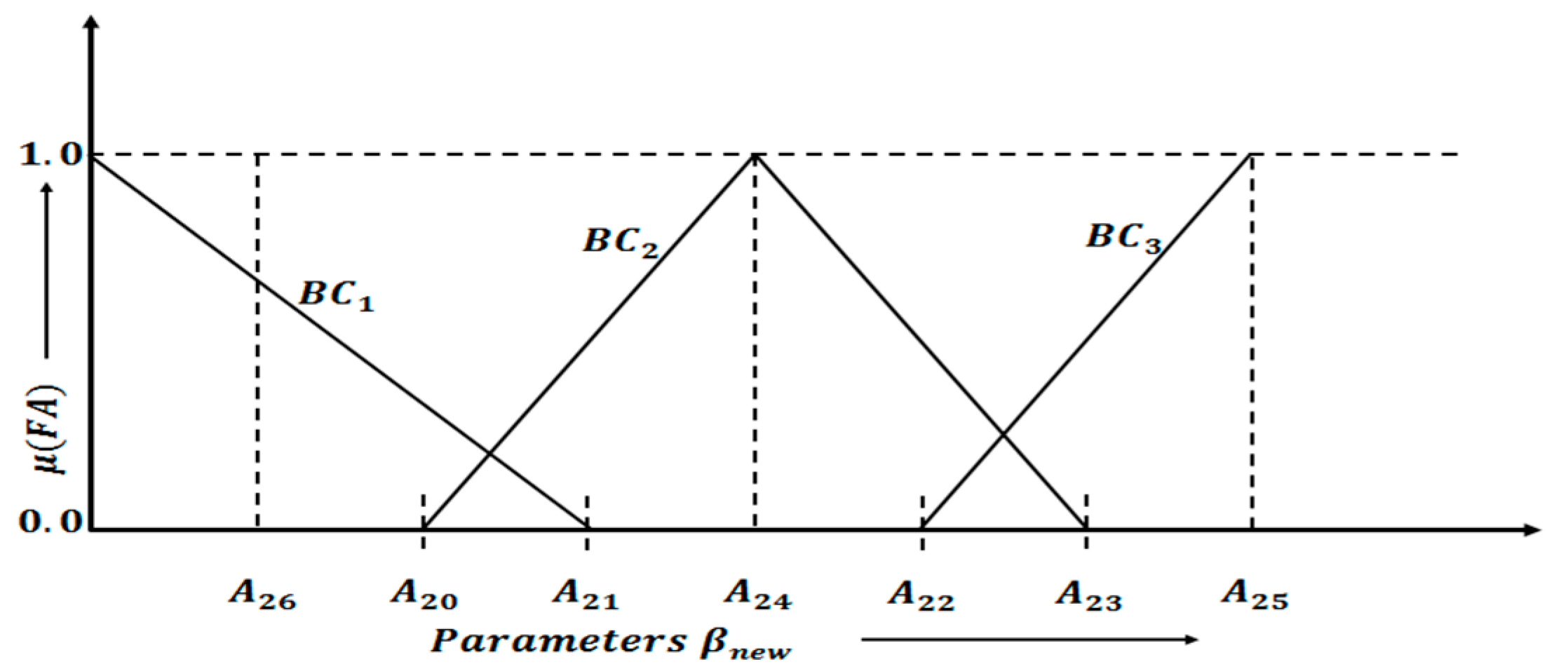
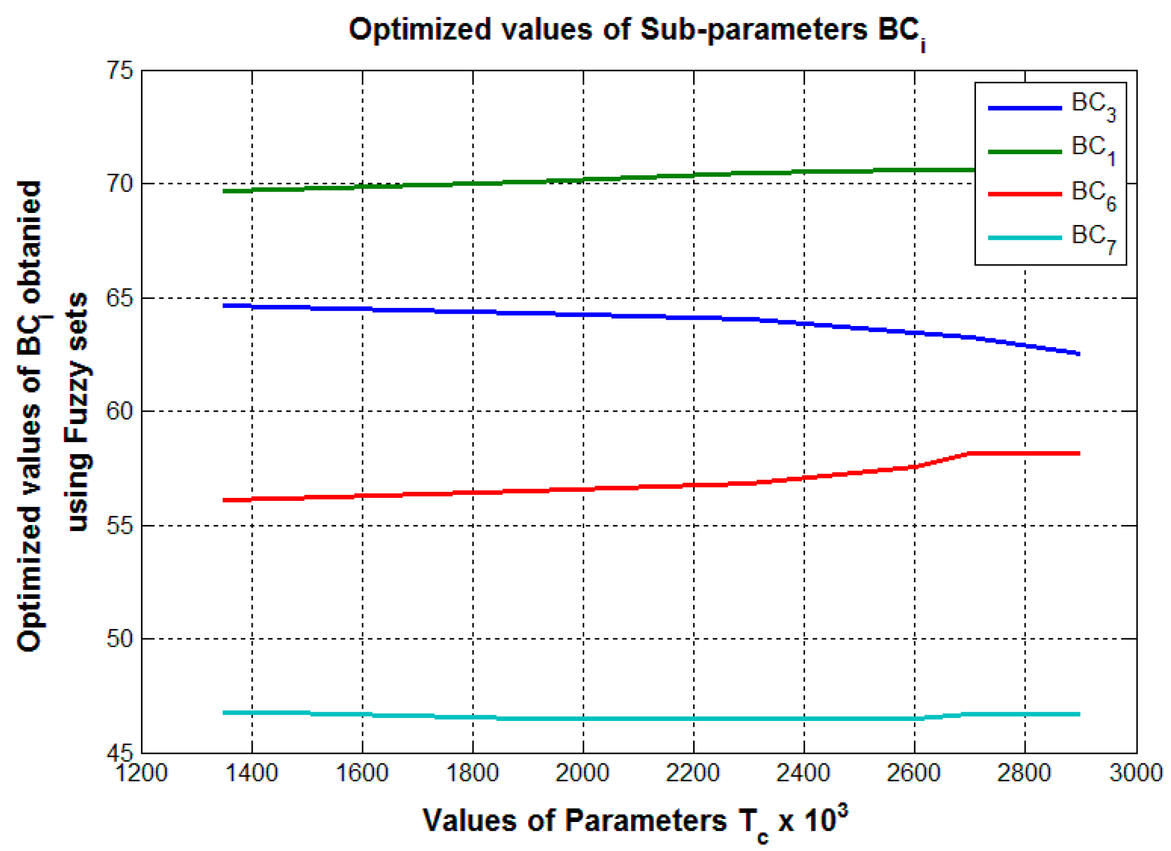
The Combined_desired_value is represented by the following equation [35]:
k = 1 M P k ( combined_desired_value + P L ) .
The classical Lagrangian multiplier method is employed on a sample data, which is assumed for testing purposes as given in [30,31,32,33,35]:
α 1 = 0.0089 α 2 = 0.00741 ,
β 1 = 10.333 β 2 = 10.833 ,
γ 1 = 200.0 γ 2 = 240.0 ,
43.44 α new 119.16 ,
22.22 β new 70.56 ,
combined_desired_value = 150.0 .
The outputs are computed:
The optimal value of   P k : P 1 = α new , P 2 = β new .
The impact of changing weight w 1 (between the ranges 0.1–1.0) on the output values of α new as well as β new is given in Figure 4.

4. Generating Novel Sub-Parameters ( B C 1 , B C 2 , , B C 8 ) from Parameters βnew and Finding Optimal Values of Sub-Parameters Using Fuzzy Sets

The parameter β new is correlated with Conditional-Value-at-Risk (CVaR) in the proposed framework. The parameter β new used in the proposed framework has a significant role, while finding the optimal solution of the system based on the parameters α new and   β new . Since the parameter β new plays a vital role in decision-making for selecting the optimal solution of the proposed framework, it becomes quite essential to bifurcate this parameter into sub parameters. These sub parameters are associated with uncertainty in their values. The representation of these sub parameters using three fuzzy sets is provided, which uses the following sets: Fuzzy Set A, Fuzzy Set B 1 and Fuzzy Set B 2 . There are eight sub parameters viz. BC 1 , BC 2 , , BC 8 . Each of these sub parameters is associated with one of the above-mentioned Fuzzy Sets. A description of association of these sub parameters with fuzzy sets is given below:
The range used for parameter β new as used in the model is 46.5 to 70.56.
  • Fuzzy Set A is used when the value of parameter β_new lies in Category A
    Category A: A0 ≤ βnew ≤ A25,
    where A25 is the value = 70.5697 and A0 is the value = 61.5669.
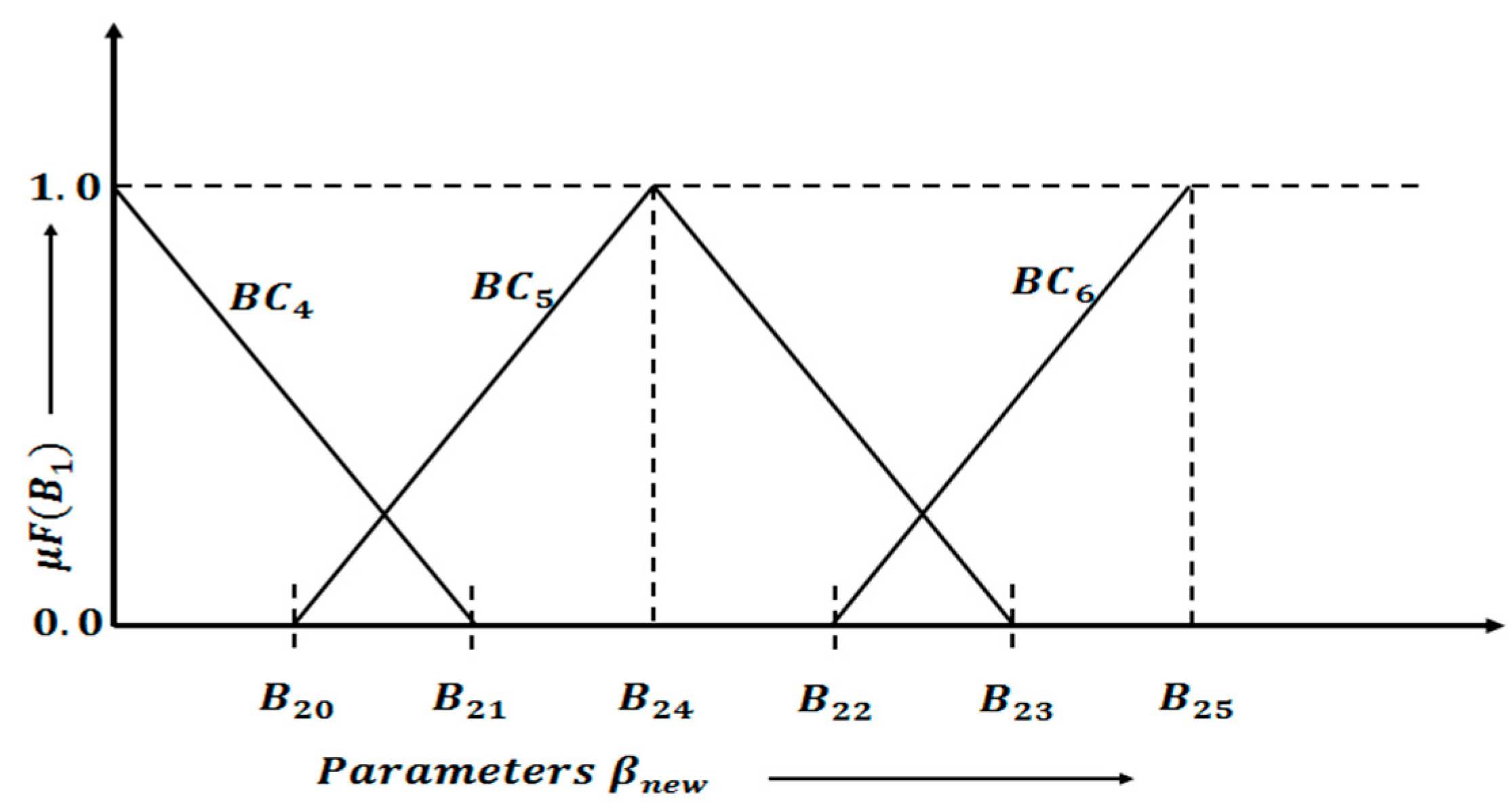
  • Fuzzy Set B1 is used when the value of parameter β n e w lies in Category B
    Category B: B20 ≤ βnew ≤ B25,
    where B20 is the value = 51.3820 and B25 is the value = 58.1558.
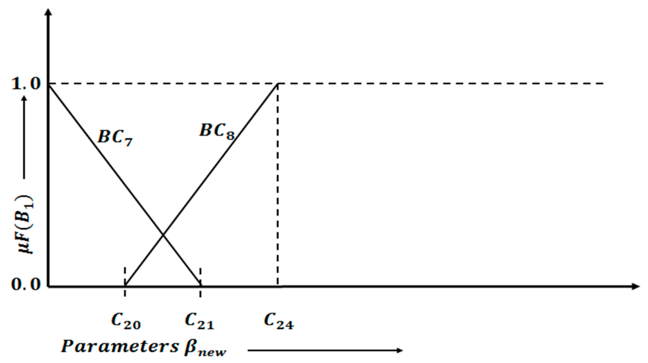
  • Fuzzy Set B2 is used when the value of parameter β n e w lies in Category C
    Category   C :   C 20 β new   C 24 ,
    where C 20 is the value = 47.2518 and B 25 is the value = 48.0185.
Let S 1 , S 2 , , S 8 denote the membership values from these fuzzy sets associated with sub parameters   BC 1 , BC 2 , , BC 8 , respectively, i.e., membership value of sub parameters BC 1 in fuzzy set A is represented by parameter S 1 :
μ ( BC i ) = S i    i = 1 , 2 , , 8 .
To find the optimal values S 1 , S 2 , , S 8 , the Lagrangian Multiplier method is employed. The minimization problem using the Lagrangian Multiplier is formulated below:
T c = Parameter representing total cost associated with parameters S 1 , S 2 , , S 8 ,
T c = i = 1 8 S i    i = 1 , 2 , , 8 ,
S i =   μ ( BC i )    i = 1 , 2 , , 8 .
The Lagrangian Multiplier method is used to find the solution of the above-mentioned minimization problem. The coding of the program is done using C-language. A flow graph for the process Tc is given in Figure 5.
It may be noted that triangular membership functions are used for   μ ( FA ) , μ ( B 1 ) and μ ( B 2 ) . A graphical representation of the triangular membership functions is shown in Figure 6, Figure 7 and Figure 8 and definitions of these membership functions are given in [30,31,32,35]. The selection of triangular membership function in fuzzy sets is justified in view of the data values of the parameters used in the methodology. The parameter has the highest membership value when the value of parameter is near its mean-value. If the value of the parameter deviates from this mean-value, the membership value is assumed to have linear behavior. This selection of triangular membership function is mainly for modeling the membership values with the help of mathematical equations in the methodology, although other types of membership functions may be employed instead of the triangular membership function depending upon the structure of the chosen application.

4.1. Description of Various Equations Used in Fuzzy Sets

The various equations used in describing a fuzzy set for a specific category are given below.

4.1.1. Category A: Fuzzy Set-A

Here, A 2 is representing the value of parameter   β new :
μ ( BC 1 ) = { 1 ; A 2 = 0.0 A 21 A 2 A 21 A 26 ; 0 < A 2 < A 21 0 ; A 2 A 21 ,
μ ( BC 2 ) = { 1 ; A 2 = A 24 A 24 A 2 A 24 A 20 ; A 20 < A 2 < A 24 0 ; A 2 A 20 A 23 A 2 A 23 A 24 ; A 24 < A 2 < A 23 ,
μ ( BC 3 ) = { 1 ; A 2 A 25 A 25 A 2 A 25 A 22 ; A 22 < A 2 < A 25 0 ; A 2 A 22 .

4.1.2. Category B: Fuzzy Set-B1

The equations for membership value of fuzzy set B1 are given next.
μ ( BC 4 ) = { 1 ; A 2 = 0.0 B 21 A 2 B 21 0 ; 0 < A 2 < B 21 0 ; A 2 B 21 ,
μ ( BC 5 ) = { 1 ; A 2 = B 24 B 24 A 2 B 24 B 20 ; B 20 < A 2 < B 24 0 ; A 2 < B 20 B 23 A 2 B 23 B 24 ; B 24 < A 2 < B 23 ,
μ ( BC 6 ) = { 1 B 25 A 2 B 25 B 22 0 ; A 2 B 25 ; B 22 < A 2 < B 25 . ; A 2 B 22  

4.1.3. Category C: Fuzzy Set- B 2

The equations for membership value of fuzzy set B2 are given next.
μ ( BC 7 ) = { 1 ; A 2 = 0.0 C 21 A 2 C 21 0 ; 0 < A 2 < C 21 0 ; A 2 C 21 ,
μ ( BC 8 ) = { 1 ; A 2 = C 24 C 24 A 2 C 24 C 20 ; C 20 < A 2 < C 24 0 ; A 2 C 20 .
The inputs used are:
(a)
The values of cost-coefficients g i , h i as used in the following equation:
Minimize   T c = i = 1 8 g i s i 2 + h i s i = i = 1 8 CS i .
(b)
The values of these coefficients are given in Table 4.
(c)
The specified value of T c .
The outputs computed are:
The optimal values of outputs Parameters ( S 1 , S 2 , , S 8 ) which are computed using the Lagrangian Multiplier method:
S i = μ ( BC i )    i = 1 , 2 , , 8 .

4.2. Mathematical Modeling of Module for Computing Sub Parameters

The maximum and minimum values of S i is represented by the following equation:
S i min     S i     S i max .
Minimize   T c =   w 1 s 1 + w 2 s 2 + + w 8 s 8 ,
T c = i = 1 8 CS i ,
T c = i = 1 8 W i S i CS i = W i S i , i = 1 8 W i S i = Specified_Limit , W = [ 0.89 , 0.75 , 0.75 , 0.4 , 0.4 , 0.4 , 0.1 , 0.1 , 0.1 , 0.1 ] .
The weights used in the program are listed above. The chosen list shows a sample list selected for testing purposes:
Minimize T c = i = 1 8 CS i T c = i = 1 8 g i s i 2 + h i s i , Subject to i = 1 8 W i S i = Specified Limit , where , CS i = g i s i 2 + h i s i .

4.3. Equations for Parameters C S i (i = 1 to 8)

The equations used for parameters CS i are given below.
Parameter   CS i = W i S i ,
CS 1 = ( A 21 BC 1 ) × W 1 J 1 , 0 S 1 0.89 ,
J 1 = ( A 21 A 26 ) ,
CS 2 = ( BC 2 A 20 ) × W 2 J 2 , 0 S 2 0.75 ,
J 2 = ( A 24 A 20 ) ,
CS 3 = ( BC 3 A 22 ) × W 3 J 3 , 0 S 3 0.75 ,
J 3 = ( A 25 A 22 ) ,
CS 4 = ( B 21 BC 4 ) × W 4 J 4 , 0 S 4 0.4 ,
J 4 = ( B 21 B 26 ) ,
CS 5 = ( BC 5 B 20 ) × W 5 J 5 , 0 S 5 0.4 ,
J 5 = ( B 24 B 20 ) ,
CS 6 = ( BC 6 B 22 ) × W 6 J 6 , 0 S 6 0.4 ,
J 6 = ( B 25 B 22 ) ,
CS 7 = ( C 21 BC 7 ) × W 7 J 7 , 0 S 7 0.1 ,
J 7 = ( C 21 C 26 ) ,
CS 8 = ( BC 8 C 20 ) × W 8 J 8 , 0 S 8 0.1 ,
J 8 = ( C 24 C 20 ) .

4.4. Description of Different Outputs of the Module for Sub-Parameters

The parameter T c represents total cost and is defined using Equation (36). Different inputs values of parameter T c are selected and the optimal values of parameters CS i are computed using the Lagrangian Multiplier method. Here, the parameter CS i represents values   W i S i , where W i is weight used in the program. The values of parameters CS 2 and CS 5 are fixed at their maximum values of 0.210 and 0.310 in the program. Now, the values of sub-parameters BC i are computed using Equations (37)–(44). The outputs of sub-parameters are quite helpful for a portfolio optimization decision maker to choose an appropriate value of   BC i , given an input value of   T c . For example, if given input value of T c is 1.9, then the decision maker may choose the value of parameter BC 1 as 64.33. As this value of BC 1 belongs to category-A as shown in Table 5. Thus, the selector may choose category-A for the parameter   β new . The minimum and maximum values of S i are given in Table 6. The output values of CS i computed using the Lagrangian Multiplier method for different input values of parameter   T c are shown in Table 7. The output values of sub-parameters BC i are given in Table 8 and the variations in the values of   BC 1 , BC 3 , BC 6 and BC 7 , with a change in the value of parameter T c (Scale used = Value × 10 3 ) is shown in Figure 9.

5. Need for Design of a Model Using Fuzzy Logic

A decision maker can keep fuzzy or vague objectives for portfolio selection. Since the decision about an objective lacks exactness, it is desirable to contemplate a fuzzy model for selecting an appropriate portfolio. A fuzzy set makes use of equations, which are called membership function in a fuzzy set and the value of this membership function can lie between 0 and 1.
If this membership value is 0, then it implies that the object is impertinent with the given fuzzy set. If this membership value is 1, then it implies that the object is fully compatible with the given fuzzy set. A membership function μ ( F i ) may be considered for the objective, which is used in portfolio selection. We are considering a strictly monotonic decreasing (or monotonic increasing) and continuous membership function μ ( F i ) [31,32,33,36]:
μ ( F i ) = { 1 ; F i F i min F i max F i F i max F i min ; F i min < F i < F i max 0 ; F i F i max .
To analyze the performance of the proposed model for fuzzy inference system, the model is coded in Matlab and results are used in a C program.
We use the following rules in the fuzzy inference system:
  • Input 1 = F 11 , Input 2 = F 12 , Input 3 = F 21 , Input 4 = F 22
  • Rule 1: IF   ( F 11   is Low   &   F 12   is Low   &   F 21   is Low   & F 22   is Low )   THEN   ( Output   is   Low )
  • Rule 2: IF   ( F 11   is Low   &   F 12   is Low   &   F 21   is   Average   & F 22   is   Average )   THEN   ( Output   is   Low )
  • Rule 3: IF   ( F 11   is   Average   &   F 12   is   Average   &   F 21   is Low   &   F 22   is Low )   THEN   ( Output is Average )
  • Rule 4: IF   ( F 11   is Average   &   F 12   is Average   &   F 21   is Average   & F 22   is Average )   THEN   ( Output is Average )
  • Rule 5: IF   ( F 11   is High   &   F 12   is High   &   F 21   is High   &   F 22   is High )   THEN   ( Output is High )
  • Rule 6: IF   ( F 11   is Low   &   F 12   is Average   &   F 21   is Low   & F 22   is Average )   THEN   ( Output is Average )
  • Rule 7: IF   ( F 11   is Low   &   F 12   is High   &   F 21   is Low   & F 22   is High )   THEN   ( Output is High )
  • Rule 8: IF   ( F 11   is Average   &   F 12   is High   &   F 21   is Average   &   F 22   is High )   THEN   ( Output is High ) .

6. New Model Using Modifications in ANFIS: Six-Layered Structure

Fuzzy inference systems require a prior knowledge about the data of a problem. The designing of the complicated rules of fuzzy inference system is arduous in understanding. Similarly, neural networks also have a drawback related to the design of the complicated structure of the network. The design involving this complicated structure is hard to understand. Due to these reasons, the need for neural fuzzy systems came into existence. A neural fuzzy system keeps the advantages of fuzzy systems and neural networks. This system also overbalances the disadvantages of fuzzy systems and neural networks. This system relies on creating information about a problem by a training network in the neural inference system. The drawback of the complicated structure of the neural network is outweighing by defining linguistic variables. These linguistic variables are suitable for explaining the outputs. The proposed model, used in this paper, makes use of modified adaptive neuro-fuzzy inference system and it has six layers.
Layer 1: This Layer contains adaptive nodes with node functions as:
P_spot 1 i = μ A i ( F 1 )   for   i = 1 , 2 ,
P_spot 1 i = μ B i 2 ( F 2 )   for   i = 3 , 4 ,
where F 1 and F 2 are input nodes, A and B are the linguistic labels, and μ ( F 1 ) and μ ( F 2 ) are the membership functions. Different membership functions are used in the model where it is assumed that μ ( F i ) is a strictly monotonically decreasing and continuous function defined as:
a 1 = F 1 max ,   b 1 = F 1 min ,   a 2 = F 2 max ,   b 2 = F 2 min ,
where   c 1 = 1 ,   c 2 = 1 ,
μ ( F 1 ) = { c 1 ; F 1 b 1 a 1 F 1 a 1 b 1 ; b 1 < F 1 < a 2 0 ; F 1 a 2 ,
( F 2 ) = { c 2 ; F 2 b 2 a 2 F 2 a 2 b 2 ; b 2 < F 2 < a 2 0 ; F 2 a 2 ,
where a i , b i , and   c i are the parameters. The membership function varies while the values of parameters are changing.
Layer 2: Every node i in this layer is computed using the product of incoming signals and parameter j i . It outputs the product out by Equations (42) and (43). The weights j 1 , j 2 , j 3 and j 4 are used with T 1 , T 2 , T 3 and T 4 , respectively. Parameters T 1 and T 2 are being used with node μ B 1 _ F 2 , whereas parameters T 3 and T 4 are being used with node μ B 2 _ F 2 .
Case 1: If j 1 has a greater value than j 2 and j 3 has a greater value than j 4 i.e., j 1 > j 2 , j 3 > j 4 .
The assumed values of j 1 and j 2 are given below:
j 1 = 0.6 ,   j 2 = 0.45 , w 1 a = μ A 1 F 1     j 1     μ B 1 _ F 2 ,   w 1 b = μ A 1 F 1     j 2     μ B 1 _ F 2 , T 1 = j 1     μ B 1 _ F 2 ,   T 2 = j 2     μ B 1 F 2 , w 1 = w 1 a + w 1 b .
The assumed values of j 3 and j 4 are given below:
j 3 = 0.56 ,   j 4 = 0.44 , w 2 a = μ A 2 F 1     j 3     μ B 2 _ F 2 ,   w 2 b = μ A 2 F 1     j 4     μ B 2 F 2 , T 3 = j 3     μ B 2 _ F 2 ,   T 4 = j 4     μ B 2 F 2 , w 2 = w 2 a + w 1 b .
Case 2: If j 2 has a greater value than j 1 and j 4 has a greater value than j 3 :
j 1 < j 2 ,    j 1 = 0.45   and   j 2 = 0.59 , j 3 < j 4 ,    j 3 = 0.40   and   j 4 = 0.59 .
Layer 3: Every node i in this layer is a square node labelled P_spot 3ia and P_spot 3ib . The i-th node calculates the ratios w ia i = 1 2 w ia and w ib i = 1 2 w ib for i = 1, 2 by (44) and (46):
P_spot 31 a = w 1 a ( w 1 a + w 2 a ) ,   P_spot 32 a = w 2 a ( w 1 a + w 2 a ) ,
w 1 a   bar = P_spot 31 a ,   w 2 a   bar = P_spot 32 a ,
P_spot 31 b = w 1 b ( w 1 b + w 2 b ) ,   P_spot 32 b = w 2 b ( w 1 b + w 2 b ) ,
w 1 b   bar = P_spot 31 b ,   w 2 a   bar = P_spot 32 b .
Layer 4: Every node i in this layer is a square node with a node function w ibar = w iabar + w ibbar :
w 1   bar = w 1 a   bar + w 1 b   bar ,   w 2   bar = w 2 a   bar + w 2 b   bar .
Layer 5: Every node i in this layer is a square node with a node function ϖ · f ai , for i = 1, 2
P_spot 4 i = ϖ · f ai ,   for   i = 1 , 2 ,
where f a 1 and f a 2 are the fuzzy IF-THEN rules given below:
  • Rule 1: IF   F 1   is   P_spot 11   and   F 2   is   P_spot 13   THEN   f a 1 = p 1 F 1 + q 1 F 2 + r 1 ,
  • Rule 2: IF   F 1   is   P_spot 12   and   F 2   is   P_spot 14   THEN   f a 2 = p 2 F 1 + q 2 F 2 + r 2 ,
where p i , q i and r i are the parameters set, referred to as the consequent parameters. Parameters are P 1 , P 2 and P 3 . Scale used in the layer = Value of the parameter/1000. The following limits are used in the layer:
P 1 min = 0.15 ,   P 1 max = 0.6 ,   P 2 min = 0.1 ,   P 2 max = 0.4 ,   P 3 min = 0.05 ,   P 3 max = 0.2 .

Proposed Modifications in Fifth Layer (Layer 5) for Modified ANFIS Using the Cuckoo Intelligence Algorithm

This portion puts forth the details of the proposed modifications in the fifth layer of modified ANFIS. The modifications are centred around optimizing parameters that are being used in two rules viz. Rule 1 and Rule 2 employed in the existing Fifth layer. A newly framed scheme has been proposed in the following section that optimizes the values of parameters in these two rules by employing cuckoo intelligence algorithm.

General Framework of the Modification

The existing Fifth layer is based upon computing the values of nodes f a 1 and f a 2 as given below:
  • Rule 1: f a 1 = p 1 F 1 + q 1 F 2 + r 1 ,
  • Rule 2: f a 2 = p 2 F 1 + q 2 F 2 + r 2 .
The different parameters identified in these rules are listed below:
Parameters: p 1 , p 2 , q 1 , q 2 , r 1 and r 2 .
The optimization of computed values of these parameters is felt in view of the outputs obtained by abovementioned rules. If we associate cost parameters for the given parameters p 1 and p 2 , then these costs can be modeled accuretly using the following quardatic equations:
Optimized value used in the node   ( p 1 ) = a 1 p 1 2 + b 1 p 1 + c 1 ,
Optimized value used in the node   ( p 2 )   =   a 2 p 2 2 + b 2 p 2 + c 2 .
Here, a new parameter p 3 is assumed that is correlated with sum of three parameters (is that p 1 + p 2 + p 3 ). The cost for the parameter can be specified as:
Optimized   value   used   in   the   node   ( p 3 ) = a 3 p 3 2 + b 3 p 3 + c 3 .
If this sum is specified example 850/1000 in the problem, the value of the p 3 is calculated as given below:
p 3 = 850 1000 ( p 1 + p 2 ) .
This value of parameter sum can be chosen by the user of the portfolio and gives a decision-making capability to the user.
The algorithm will optimize three values viz. ( p 1 , p 2 and p 3 ) if the sum is specified. The optimized model for computing values of p 1 , p 2 and p 3 can be described by Equations (57)–(59).
A new scheme has been put forth as described below:
Rule   1   ( modified ) :   fa 1 = α 1 F 1 + β 1 F 2 + γ 1 ,
where the values of coefficients are specified below:
α 1 = p 1 + p 2 2 ;   β 1 = p 1 p 1 + p 2 + p 3 ;   γ 1 = p 1 p 2 × 0.01 ,
Rule   2   ( modified ) :   fa 2 = α 2 F 2 + β 2 F 2 + γ 2 ,
where the values of coefficients are specified below:
α 2 = p 2 + p 3 2 ;   β 2 = p 2 p 1 + p 2 + p 3 ;   γ 2 = p 2 p 3 × 0.01 .
The optimizied values of the parameters p 1 , p 2 and p 3 are computed by running cuckoo intelligence algorithm and these values are given in Table 9 and Table 10. The coefficients used in modified Fifth layer and described by Equations (60) and (61).
Layer 6: The single node in this layer is a circle node, which computes the summation of all incoming signals as the overall output (see (62)):
P spot 5 i = f aout = ϖ · f ai = overalloutput ,
f aout = ϖ 1 · f a 1 + ϖ 2 · f a 2 = w 1 w 1 + w 2 · f a 1 + w 2 w 1 + w 2 · f a 2 ,
f aout = ( ϖ 1 · F 1 ) P 1 + ( ϖ 1 · F 2 ) q 1 + ( ϖ 1 ) r 1 + ( ϖ 2 · F 1 ) P 2 + ( ϖ 2 · F 1 ) P 2 + ( ϖ 2 · F 2 ) q 2 + ( ϖ 2 ) .
A general architure of the modified ANFIS is given in Figure 10.

7. Performance Analysis and Experimental Results

7.1. Discussion on Modifications of the Range Used within a Cuckoo Intelligence Algorithm (Layer 5 of Modified 6 Layered ANFIS)

The Cuckoo Intelligence algorithm is being used to find the optimal values of three parameters viz. p 1 , p 2 and p 3 . The values of these parameters are used to find the outputs of Rule 1 and Rule 2 , which are currently used in Layer 5 of modified ANFIS model.
Scale used for describing the limits for p 1 , p 2 and p 3 = Actual value/1000.
The following new ranges are used in the cuckoo intelligence algorithm:
  • p 1 min = 0.15 p 1 p 1 max = 0.6,
  • p 2 min = 0.1   p 2 p 2 max = 0.4,
  • P 3 min = 0.05   p 3 P 3 max = 0.2.
The output obtained by executing the cuckoo intelligence algorithm with the first set of ranges is given in Table 9. The output obtained by using new ranges that are mentioned above is given in Table 10. The optimized value obtained with new ranges in the cuckoo intelligence algorithm is 10.3241. Although the optimizied value is more with new ranges, it is justified in view of selecting more accurate limits for parameters p 1 , p 2 and p 3 . Hence, the decision maker may choose an appropriate range of limits for these parameters and may obtain an accurate optimal value.
The computed values of the coefficients used in the fifth layer of modified ANFIS are given in Table 11. The outputs obtained for the first layer (layer 1) of existing ANFIS and modified ANFIS is given in Table 12. As shown in this table membership values of F 1 and F 2 are same as values of A 1 and A 2 in the existing ANFIS whereas, the output values of layer 2 are different in the new modified model. Thus, corresponding output values of layer 3 is also different consequently. The output of existing ANFIS (consisting of layer 5) is given in Table 13. A comparison of different outputs obtained for second layer (layer 2), fifth layer (layer 5) and last layer (layer 6) of modified ANFIS is given in Table 14, Table 15 and Table 16. As evident from the outputs given in Table 15, those changes incorporated in the fifth layer (layer 5) result in a significant change in the outputs of the last layer. If we incorporate changes in multiple layers (second and fifth layers), then the output node value of last layer (layer 6) abruptly deviates and reaches a value of 888.7410. Thus, a modified ANFIS has a significant role in determining the outputs of last layer. The output of layer 6, in a modified ANFIS model, changes drastically with these modifications. Hence, the final output obtained from layer 6 of the modified ANFIS model can be used as an important index for measuring the performance of the proposed framework. This modified ANFIS model is an important tool for establishing the performance index of the proposed framework. This performance index is a significant indicator of evaluating the performance of the framework. The output values of the existing cuckoo intelligence algorithm and new ranges with the same algorithm are shown in Figure 11.

7.2. Computational Results with Analysis of ANFIS

In what follows next, we compare the outputs obtained from modified ANFIS and the existing ANFIS [18].

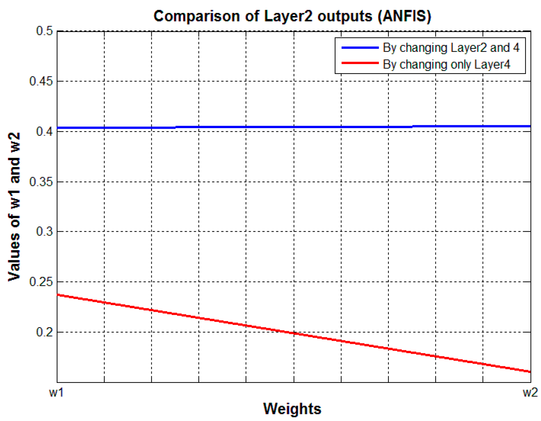
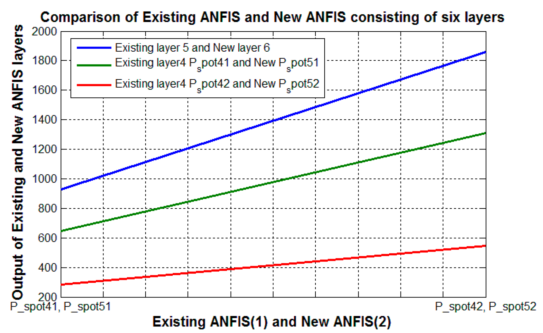
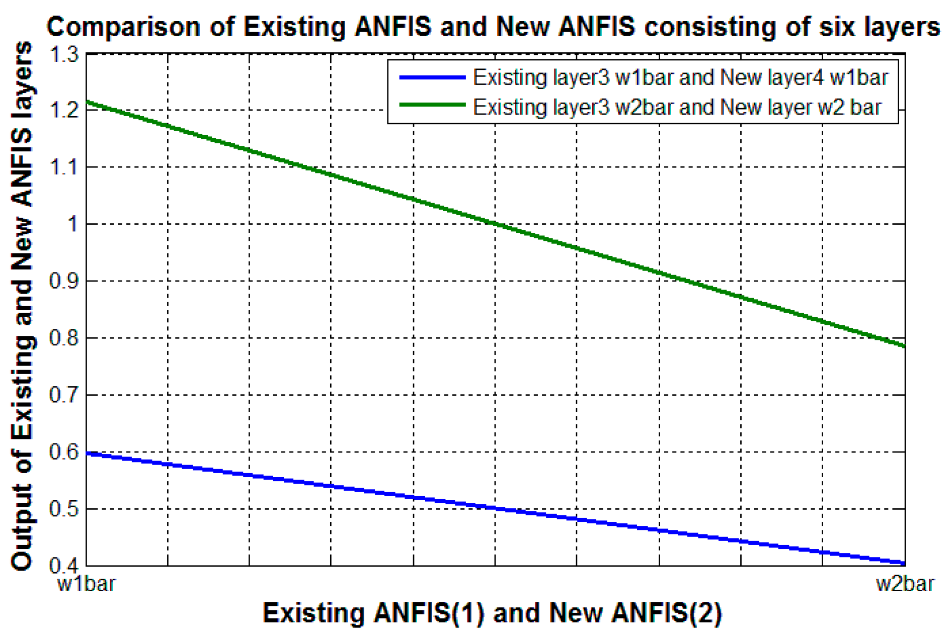
7.2.1. Comparison of Various Outputs Obtained by Changing Different Layers of ANFIS

To test the effectiveness of the ANFIS, we compare the outputs of layer 2 and layer 5 by modifying structure layer 2 and layer 5. It is evident that the output of the last layer is quite different in case we make changes in layer 5. Thus, the modification done in layer 5 has a significant role in changing the structure of the ANFIS model. In Figure 12, the cost computed using a Cuckoo Intelligence algorithm for setting the values of parameters used in layer 5 of the modified ANFIS has been given. Although, the cost is more with new ranges, but it is justified in view of selecting more accurate limits for parameters p 1 , p 2 and p 3 . Hence, the decision maker may choose an appropriate range of limits for these parameters and may obtain an accurate value of fifth layer. The output of modified ANFIS (consisting of six layers) is given in Table 14, Table 15 and Table 16. As it is evident from the data, output values of layer 2, layer 3, layer 4 and layer 5 are different from the output of the existing ANFIS model. The output f aout has a value of 1606.3 in the existing ANFIS model, whereas, in the modified ANFIS, it has values of 925.8, 1527.0 and 888.74.

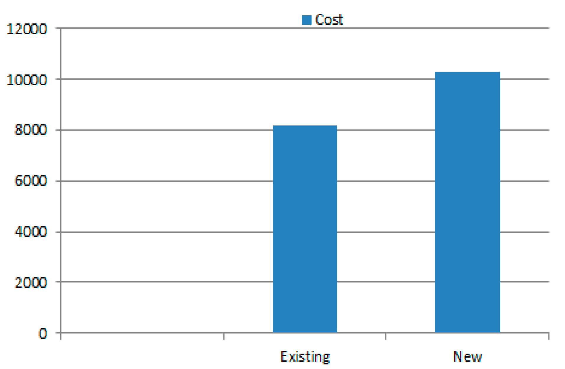
7.2.2. Comparison of Values of Output Nodes of the Last Layer in Existing and Modified ANFIS

Corresponding to the final output of modified ANFIS, as given in Table 14, Table 15 and Table 16 we find that the output of layer 6 is 888.7410 (by changing layer 2 and layer 5 simultaneously) and the output of existing ANFIS layer 5 is 1606.3 (given in Table 13). Since this output is a performance index for the ANFIS model, it can be seen that the modified ANFIS provides a very less value of this index. Hence, it is accurately modeling the different layers of the system. The output of the ANFIS system final by changing only layer 2 is 1527.0. Therefore, it has an impact on the final output compared to the output of existing ANFIS, which is 1606.3. Similarly, the output of ANFIS system by changing only layer 5 is 925.8. It is seen that the modifications done in layer 5 have a greater impact in changing the final output of ANFIS. The impact of changing layer 5 can be seen in Figure 13. The impact of changes made in layer 2 and layer 5 is shown in Figure 14. The existing output values of layer 3 nodes viz. w 1bar , w 2bar and new output values of layer 4 viz. w 1bar , w 2bar are shown in Figure 15. In addition, the new modified ANFIS obtained by changing layer 2 and layer 5 has the best evaluation performance index as the final output of layer 6. A comparison of values of the output node of last layer for modified ANFIS is given in Table 17.
A novel scheme is presented next, which is devised for computing the expected returns for 10 assets [33] after appropriately modifying the basic mean-variance model. Firstly, the return for the next month is forecasting by applying rules of thumb to approximate the trend obtained from 12 months of data [33]:
Modified   value   of   expected   return = ( ( returns   of   12   month ) + forecast   value   of   next   month ) / 13 .
This computation is performed for all the assets, thus providing the expected returns for 10 assets. The variance and co-variance are found using these 10 values of expected returns. The final outputs are obtained using expected returns and covariance. The coding is done in MATLAB The results obtained are given in Table 18, Table 19 and Table 20. The impact of change on expected returns and allocation is depicted in the tables:
Final   value   of   expected   return = Modified   value   of   expected   return + ( Scaling factor 1     Decision parameter ) .
Firstly, the decision parameter used is the value of Tc (Tc = 2.3) and scaling_factor1 is taken as 1 × 10⁻². The output obtained are given in Table 18. Next, the decision parameter used is the value of TA1 (TA1 = 888.7410) and scaling_factor1 is taken as 1 × 10⁻⁴. The output obtained are given in Table 19. Here, TA1 is representing the output of modified ANFIS by changing Layer 2 and Layer 5 simultaneously. Lastly, the decision parameter used is the value of TA2 (TA2 = 1606.3) and scaling_factor1 is taken as 1 × 10⁻⁵. The output obtained are given in Table 20. Here, TA2 is representing the output of existing ANFIS. As shown in Table 18, Table 19 and Table 20, the values of expected returns as well as the allocation of 10 assets is changed even though the decision parameter is chosen to be nominally based upon either Tc, TA1 or TA2. While comparing the values of expected returns and allocation of assets, it is observed that these values are more with decision parameter TA1 as compared with values obtained with values obtained with Tc, whereas these values are less with decision parameter TA2 when compared with values obtained with Tc. It is evident from these observed values that the proposed framework provides a necessary model for including uncertainty in the form of newly parameters given by α new and β new . Furthermore, the modified ANFIS has the ability to modify the expected returns based upon its output.

7.2.3. Economic Significance of the ANFIS Methodology for Additional Constraints

The additional constraints permit optimization algorithms to account for the random nature of the risk, which unavoidably affects the expected return and which can cause significant changes in the values of expected returns for the multi-asset data set. A comparison of the expected return is provided in Table 21. As evident from the values given in the table, the inclusion of additional constraints allows the investor with more accurate modelling for risk-based portfolio selection, thus generating better values of the expected returns. Hence, this modified ANFIS increases the accuracy of the presently available ANFIS structure, in terms of the risk-based approach.

8. Conclusions

This paper has formulated, in a formal way, the portfolio based on two newly parameters. The minimization model is further framed by considering optimal values of the costs associated with these newly parameters. Here, a modern scheme is presented, in order to correlate the derived parameters with output parameters of the basic mean-variance model and Conditional-Value-at-Risk. This recent technique is quite advantageous for finding optimal values of the newly parameters as well as helping the investor in selecting an optimal portfolio. Another useful attribute of the scheme is that it can be easily implemented online. Another significant scheme is contemplated to formulate sub parameters, which are used for selecting an appropriate value of parameter β new . This scheme is framed by making use of fuzzy sets, which are appropriate in accommodating uncertainty in the values of sub parameters. Such a novel scheme is thoroughly adaptable for the decision-making process of the investor in order to select a more accurate value of parameter β new . Finally, a six-layered structure of ANFIS model is given in the paper. The changes incorporated in the existing ANFIS model are described here and the outputs obtained from the modified ANFIS are provided in the paper. The obtained result signifies contribution of the new structure as well as the impact of modifications made in different layers. Lastly, a comparison is made between the existing ANFIS model and the modified ANFIS model. The output of the modified model is drastically different from the output of the existing model. This can be harnessed as an indicator for estimating the performances of the models. Thus, the designer has an essential tool to appraise the performance of the model.
The solution obtained for the proposed model with respect to multiobjective functionals can be investigated with this methodology and additional objectives can be added as future work. Nowadays, big data analytics play a vital role in handling information. Thus, this is another dimension for investigating the methodology. The role of user-satisfaction might be studied along with the methodology.

Author Contributions

All authors have devised and put forth the main structure of the framework. C.K. provided the basic details of the framework and implemented different algorithms. C.K. and M.N.D. analyzed, compared and plotted the different outputs.

Funding

This publication is an outcome of the R&D work undertaken project under the Visvesvaraya PhD Scheme of Ministry of Electronics and IT, Government of India, being implemented by Digital India Corporation.

Conflicts of Interest

The authors declare no conflicts of interest.

References

  1. Markowitz, H.M. Portfolio Selection. J. Financ. 1952, 7, 77–91. [Google Scholar]
  2. Huang, X. Fuzzy chance-constrained portfolio selection. Appl. Math. Comput. 2006, 177, 500–507. [Google Scholar] [CrossRef]
  3. Gupta, P.; Inuiguchi, M.; Mehlawat, M.K.; Mittal, G. Multiobjective credibilistic portfolio selection model with fuzzy chance-constraints. Inf. Sci. 2013, 229, 1–17. [Google Scholar] [CrossRef]
  4. Huang, X. Portfolio selection with fuzzy returns. J. Intell. Fuzzy Syst. 2007, 18, 383–390. [Google Scholar]
  5. Huang, X. Mean-semivariance models for fuzzy portfolio selection. J. Comput. Appl. Math. 2008, 217, 1–8. [Google Scholar] [CrossRef]
  6. Li, X.; Qin, Z.; Kar, S. Mean-variance-skewness model for portfolio selection with fuzzy returns. Eur. J. Oper. Res. 2010, 202, 239–247. [Google Scholar] [CrossRef]
  7. Huang, X. Risk curve and fuzzy portfolio selection. Comput. Math. Appl. 2008, 55, 1102–1112. [Google Scholar] [CrossRef]
  8. Gupta, P.; Mittal, G.; Mehlawat, M.K. Multiobjective expected value model for portfolio selection in fuzzy environment. Optim. Lett. 2012, 7, 1765–1791. [Google Scholar] [CrossRef]
  9. Mehlawat, M.K.; Gupta, P. Fuzzy Chance-Constrained Multiobjective Portfolio Selection Model. IEEE Trans. Fuzzy Syst. 2014, 22, 653–671. [Google Scholar] [CrossRef]
  10. Wang, B.; Wang, S.; Watada, J. Fuzzy-Portfolio-Selection Models with Value-at-Risk. IEEE Trans. Fuzzy Syst. 2011, 19, 758–769. [Google Scholar] [CrossRef]
  11. Rockafellar, R.T.; Uryasev, S. Optimization of conditional value-at-risk. J. Risk 2000, 2, 21–41. [Google Scholar] [CrossRef] [Green Version]
  12. Yao, H.; Li, Z.; Lai, Y. Mean–CVaR portfolio selection: A nonparametric estimation framework. Comput. Oper. Res. 2013, 40, 1014–1022. [Google Scholar] [CrossRef]
  13. Yan, W.; Miao, R.; Li, S. Multi-period semi-variance portfolio selection: Model and numerical solution. Appl. Math. Comput. 2007, 194, 128–134. [Google Scholar] [CrossRef]
  14. Yan, W.; Li, S. A class of multi-period semi-variance portfolio selection with a four-factor futures price model. J. Appl. Math. Comput. 2008, 29, 19–34. [Google Scholar] [CrossRef]
  15. Najafi, A.A.; Mushakhian, S. Multi-stage stochastic mean–semivariance–CVaR portfolio optimization under transaction costs. Appl. Math. Comput. 2015, 256, 445–458. [Google Scholar] [CrossRef]
  16. Freitas, F.D.; Souza, A.F.D.; Almeida, A.R.D. Prediction-based portfolio optimization model using neural networks. Neurocomputing 2009, 72, 2155–2170. [Google Scholar] [CrossRef]
  17. Alizadeh, M.; Rada, R.; Jolai, F.; Fotoohi, E. An adaptive neuro-fuzzy system for stock portfolio analysis. Int. J. Intell. Syst. 2010, 26, 99–114. [Google Scholar] [CrossRef]
  18. Svalina, I.; Galzina, V.; Lujic, R.; Šimunovic, G. An adaptive network-based fuzzy inference system (ANFIS) for the forecasting: The case of close price indices. Expert Syst. Appl. 2013, 40, 6055–6063. [Google Scholar] [CrossRef]
  19. Chen, Y.-S.; Cheng, C.-H.; Chiu, C.-L.; Huang, S.-T. A study of ANFIS-based multi-factor time series models for forecasting stock index. Appl. Intell. 2016, 45, 277–292. [Google Scholar] [CrossRef]
  20. Hasuike, T.; Ishii, H. A portfolio selection problem with type-2 fuzzy return based on possibility measure and interval programming. In Proceedings of the IEEE International Conference on Fuzzy Systems, Jeju Island, South Korea, 20–24 August 2009. [Google Scholar]
  21. Pai, G.A.V. Fuzzy Decision Theory Based Metaheuristic Portfolio Optimization and Active Rebalancing Using Interval Type-2 Fuzzy Sets. IEEE Trans. Fuzzy Syst. 2017, 25, 377–391. [Google Scholar] [CrossRef]
  22. Pai, G.V.; Michel, T. Metaheuristic multi-objective optimization of constrained futures portfolios for effective risk management. Swarm Evol. Comput. 2014, 19, 1–14. [Google Scholar] [CrossRef]
  23. Pai, G.A.V.; Michel, T. Fuzzy decision theory based optimization of constrained portfolios using metaheuristics. In Proceedings of the IEEE International Conference on Fuzzy Systems, Hyderabad, India, 7–10 July 2013. [Google Scholar]
  24. Hassanzadeh, F.; Collan, M.; Modarres, M. A Practical Approach to R&D Portfolio Selection Using the Fuzzy Pay-Off Method. IEEE Trans. Fuzzy Syst. 2012, 20, 615–622. [Google Scholar]
  25. Nguyen, T.T.; Gordon-Brown, L.; Khosravi, A.; Creighton, D.; Nahavandi, S. Fuzzy Portfolio Allocation Models Through a New Risk Measure and Fuzzy Sharpe Ratio. IEEE Trans. Fuzzy Syst. 2015, 23, 656–676. [Google Scholar] [CrossRef]
  26. Zhu, H.; Wang, Y.; Wang, K.; Chen, Y. Particle Swarm Optimization (PSO) for the constrained portfolio optimization problem. Expert Syst. Appl. 2011, 38, 10161–10169. [Google Scholar] [CrossRef]
  27. Wang, B.; Watada, J. Multiobjective particle swarm optimization for a novel fuzzy portfolio selection problem. IEEJ Trans. Electr. Electron. Eng. 2012, 8, 146–154. [Google Scholar] [CrossRef]
  28. Wang, S.; Wang, B.; Watada, J. Adaptive budget-portfolio investment optimization under risk tolerance ambiguity. IEEE Trans. Fuzzy Syst. 2017, 25, 363–376. [Google Scholar] [CrossRef]
  29. Mishra, S.K.; Panda, G.; Majhi, B. Prediction based mean-variance model for constrained portfolio assets selection using multiobjective evolutionary algorithms. Swarm Evol. Comput. 2016, 28, 117–130. [Google Scholar] [CrossRef]
  30. Brar, Y.; Dhillon, J.; Kothari, D. Genetic fuzzy logic based weightage pattern search for multiobjective load dispatch problem. Asian J. Inf. Technol. 2003, 4, 365–373. [Google Scholar]
  31. Brar, Y.; Dhillon, J.S.; Kothari, D. Multiobjective load dispatch by fuzzy logic based searching weightage pattern. Electr. Power Syst. Res. 2002, 63, 149–160. [Google Scholar] [CrossRef]
  32. Tapia, C.G.; Murtagh, B.A. Interactive fuzzy programming with preference criteria in multiobjective decision-making. Comput. Oper. Res. 1991, 18, 307–316. [Google Scholar] [CrossRef]
  33. Gupta, P.; Mehlawat, M.K.; Inuiguchi, M.; Chandra, S. Fuzzy Portfolio Optimization Advances in Hybrid Multi-Criteria Methodologies; Springer: Berlin, Germany, 2016. [Google Scholar]
  34. Padhy, N.P.; Simon, S.P. Soft Computing with MATLAB Programming; Oxford University Press: New Delhi, India, 2015. [Google Scholar]
  35. Kothari, D.P.; Dhillon, J.S. Power System Optimization; PHI Learning Private Ltd.: New Delhi, India, 2012. [Google Scholar]
  36. Rubio, J.D.J. Error convergence analysis of the SUFIN and CSUFIN. Appl. Soft Comput. 2018, in press. [Google Scholar]
  37. Lughofer, E.; Pratama, M.; Skrjanc, I. Incremental Rule Splitting in Generalized Evolving Fuzzy Systems for Autonomous Drift Compensation. IEEE Trans. Fuzzy Syst. 2018, 26, 1854–1865. [Google Scholar] [CrossRef]
  38. Rubio, J.D.J. USNFIS: Uniform stable neuro fuzzy inference system. Neurocomputing 2017, 262, 57–66. [Google Scholar] [CrossRef]
  39. Pratama, M.; Lughofer, E.; Er, M.J.; Anavatti, S.; Lim, C.-P. Data driven modelling based on Recurrent Interval-Valued Metacognitive Scaffolding Fuzzy Neural Network. Neurocomputing 2017, 262, 4–27. [Google Scholar] [CrossRef]
  40. Alder, T.; Kritzman, M. Mean–Variance versus Full-Scale Optimisation: In and Out of Sample. J. Asset Manag. 2007, 7, 302–311. [Google Scholar]
  41. Cremers, J.N.; Kritzman, M.; Page, S. Optimal Hedge Fund Allocations. J. Portf. Manag. 2005, 31, 70–81. [Google Scholar] [CrossRef]
  42. Low, R.K.Y.; Faff, R.; Aas, K. Enhancing mean–variance portfolio selection by modeling distributional asymmetries. J. Econ. Bus. 2016, 85, 49–72. [Google Scholar] [CrossRef]
  43. Kritzman, M.; Page, S.; Turkington, D. In defense of Optimization: The faculty of 1/N. Financ. Anal. J. 2010, 66, 31–39. [Google Scholar] [CrossRef]
  44. Low, R.K.Y. Vine copulas: Modelling systemic risk and enhancing higher-moment portfolio optimisation. Account. Financ. 2017. [Google Scholar] [CrossRef]
  45. Hagströmer, B.; Binner, J.M. Stock portfolio selection with full-scale optimization and differential evolution. Appl. Financ. Econ. 2009, 19, 1559–1571. [Google Scholar] [CrossRef]
  46. Rad, H.; Low, R.K.Y.; Faff, R.W. The Profitability of Pairs Trading Strategies: Distance, Cointegration, and Copula Methods. SSRN Electron. J. 2016, 16, 1541–1558. [Google Scholar] [CrossRef]
  47. Anderson, R.G.; Binner, J.M.; Elger, T.; Hagströmer, B.; Nilsson, B. Mean-Variance vs. Full-Scale Optimization: Broad Evidence for the UK; Department of Economics, Lund Universtiy: Lund, Sweden, 2008. [Google Scholar]
Figure 1. Research flowchart of the proposed framework.
Computers 07 00057 g001
Figure 2. Output of the mean-variance model.
Computers 07 00057 g002
Figure 3. Data flow graph (DAG) of optimal value of P k output parameters.
Computers 07 00057 g003
Figure 4. Output of the Lagrangian multiplier method.
Computers 07 00057 g004
Figure 5. Data flow graph (DFG) of process T c (Lagrangian multiplier method).
Computers 07 00057 g005
Figure 6. Fuzzy Set A used for computing fuzzy membership in process T c .
Computers 07 00057 g006
Figure 7. Fuzzy Set B 1 used for computing fuzzy membership in process T c .
Computers 07 00057 g007
Figure 8. Fuzzy Set B 2 used for computing fuzzy membership in process T c .
Computers 07 00057 g008
Figure 9. Optimize values of sub-parameters BC i .
Computers 07 00057 g009
Figure 10. General architecture of a new modified ANFIS.
Computers 07 00057 g010
Figure 11. Output of the cuckoo intelligence algorithm with existing ranges and new selected ranges.
Computers 07 00057 g011
Figure 12. Optimal values computed using the cuckoo intelligence algorithm.
Computers 07 00057 g012
Figure 13. Comparison of modified ANFIS (by changing the different layers).
Computers 07 00057 g013
Figure 14. Comparison of existing ANFIS and modified ANFIS consisting of six layers. (Layer 4 referred in the diagram is the fifth layer (layer 5) in the modified ANFIS).
Computers 07 00057 g014
Figure 15. Comparison of existing ANFIS and modified ANFIS consisting of six layers.
Computers 07 00057 g015
Table 1. Nodes available in different layers of existing ANFIS and modified ANFIS.
Existing ANFIS
(Number of Layers = 5)
Modified ANFIS
(Number of Layers = 6)
Inputs = F 1 , F 2
S. NoLayerNodes of Existing ANFISNodes of Modified ANFIS
1.First (Layer 1) P_spot 11 Q 11 = μ A 1 ( F 1 )
P_spot 12 Q 12 = μ A 2 ( F 1 )
P_spot 21   Q 21 = μ B 1 ( F 2 )
P_spot 22 Q 22 = μ B 2 ( F 2 )
P_spot 11 Q 11 = μ A 1 ( F 1 )
P_spot 12 Q 12 = μ A 2 ( F 1 )
P_spot 21   Q 21 = μ B 1 ( F 2 )
P_spot 22 Q 22 = μ B 2 ( F 2 )
2.Second (Layer 2) P_spot 21 Q 21 w 1 = μ A 1     μ B 2
P_spot 21 Q 21 w 2 = μ A 2     μ B 2
w 1 a = μ A 1 F 1     j 1     μ B 1 _ F 2
w 1 b = μ A 1 F 1     j 2     μ B 1 _ F 2
w 2 a = μ A 2 F 1     j 3     μ B 2 _ F 2
w 2 b = μ A 2 F 1     j 4     μ B 2 _ F 2
w 1 = w 1 a + w 1 b
w 2   = w 2 a + w 2 b
3.Third (Layer 3) P_spot 31 w 31 w ¯ 1 = w 1 ( w 1 + w 2 )
P_spot 31 w 31 w ¯ 2 = w 2 ( w 1 + w 2 )
P_spot 31 a = w 1 a ( w 1 a + w 2 a )
P_spot 32 a = w 2 a ( w 1 a + w 2 a )
P_spot 31 b = w 1 b ( w 1 b + w 2 b )
P_spot 32 b = w 2 b ( w 1 b + w 2 b )
4.Fourth (Layer 4) P spot 41 Q 41 = w ¯ 1 ( f 1 )
P spot 41 Q 42 = w ¯ 2 ( f 2 )
w 1   bar = w 1 a   bar + w 1 b   bar
w 2   bar = w 2 a   bar + w 2 b   bar
5.Fifth (Layer 5) f aout = w ¯ i · f i P_spot 41 = ϖ · f a 1
P_spot 42 = ϖ · f a 2
6.Last layerNone P spot 5 i = f aout = ϖ · f ai
Table 2. Output of the mean-variance model on sample data.
S. NoPortfolio ReturnPortfolio Weights
r 0 RiskCol.5Col.8Col.10
10.25720.16220.563000.4370
20.27750.16410.500500.4995
30.29790.16970.437900.5621
40.31830.17870.375400.6246
50.33870.19050.312800.6872
60.35900.20470.250200.7498
70.37940.22070.15540.05800.7866
80.39980.23760.04850.13760.8139
90.42020.255700.11240.8876
100.44050.2773001.000
Table 3. Output of the classical Lagrangian multiplier method (optimal values of α new and β new ).
S. No Weight   ( w 1 ) Weight   ( w 2 ) α new β new
1.1.00.0001 0 95.879970.5697
2.0.90.195.879970.5697
3.0.70.395.880070.5667
4.0.510.4997.819368.4395
5.0.50.5101.035364.9947
6.0.490.51104.329361.5669
7.0.480.52107.702758.1558
8.0.470.53111.157854.7610
9.0.460.54114.699251.3820
10.0.450.55118.320248.0185
11.0.40.6119.160647.2520
12.0.10.9119.160647.2518
Table 4. Values of the coefficient used in Lagrangian Multiplier method.
S. No g i h i
10.010.8
20.0150.9
30.020.96
40.0110.85
50.0090.88
60.0080.80
70.0070.81
80.0060.87
Table 5. Depicting the association of parameter β new with parameter BC 1 , BC 2 , , BC 8 .
S. NoCategoryRange of Values of βnewParameter BCi
1A70.56–70.56 BC 3
2A68.43–70.56 BC 2
3A61.56–64.99 BC 1
4B55.00–58.15 BC 6
5B51.52–54.76 BC 5
6B49.00–51.38 BC 4
7C47.25–48.01 BC 8
8C46.50–47.25 BC 7
Table 6. Depicting the maximum and minimum values of parameter S i .
S. No.ParameterSi minSi max
1 S 1 0.050.8
2 S 2 0.210.21
3 S 3 0.010.75
4 S 4 0.150.4
5 S 5 0.310.31
6 S 6 0.10.4
7 S 7 0.050.1
8 S 8 0.050.15
Table 7. Output values of parameters CS i computed using Lagrangian multiplier method.
S. No T c C S 1 C S 2 C S 3 C S 4 C S 5 C S 6 C S 7 C S 8
12.90.5790.2100.7500.4000.3100.4000.1000.150
22.70.4140.2100.7500.4000.3100.3650.1000.150
32.60.3550.2100.7500.4000.3100.3240.1000.150
42.30.2210.2100.6760.4000.3100.2320.1000.150
51.90.1550.2100.3930.4000.3100.1880.920.150
61.450.990.2100.1530.3360.3100.1490.700.120
71.350.880.2100.1040.3140.3100.1420.660.113
Table 8. Computed values of parameter BC i for specified value of T c .
S. No T c B C 1 B C 2 B C 3 B C 4 B C 5 B C 6 B C 7 B C 8
12.962.5169.570.5749.054.5658.1546.548.01
22.763.2269.570.5749.054.5657.8746.548.01
32.663.4769.570.5749.054.5657.5546.548.01
42.364.0569.570.4649.054.5656.8246.548.01
51.964.3369.570.0649.054.5656.4846.548.01
61.4564.5769.569.7149.3854.5656.1746.7247.82
71.3564.6169.569.6449.5154.5656.1246.7547.82
Table 9. Optimized values of parameters obtained using the cuckoo intelligence algorithm.
S. NoParametersLower LimitUpper Limit CoefficientsOptimized Values by Executing Cuckoo Intelligence Scaled Optimized ValuesOptimized Value of Fifth Layer (Layer 5)
1. p 1 150600 a 1 0.001562338.8589 8.1945
b 1 7.92 0.3388589
c 1 300
2. p 2 100400 a 2 0.00194333.7502
b 2 7.85 0.3337502
c 2 320
3. p 3 50200 a 3 0.00482127.3909
b 3 7.97 0.1273909
c 3 329
Table 10. Optimized values of parameters obtained using a cuckoo intelligence algorithm with different values of upper and lower limits.
S. NoParametersLower LimitUpper Limit CoefficientsOptimized Values by Executing Cuckoo Intelligence Scaled Optimized ValuesOptimized Value of Fifth Layer (Layer 5)
1. p 1 500800 a 1 0.001562529.70670.529706710.3241
b 1 7.92
c 1 300
2. p 2 200600 a 2 0.00194377.0130.377013
b 2 7.85
c 2 320
3. p 3 50300 a 3 0.00482171.22190.1712219
b 3 7.97
c 3 329
Table 11. Computed values of the coefficients used in the Fifth layer of the modified ANFIS.
S. NoCoefficients Used in Modified Fifth LayerValues
1. α 1 0.45335985
2. α 2 0.27411745
3. β 1 0.49140574
4. β 2 0.34975271
5. γ 1 0.01405009
6. γ 2 0.02201897
Table 12. Output of the first layer (layer 1) in existing and modified ANFIS.
Selected Layer in Existing and Modified ANFISNodes Used in the Selected Layer Chosen Values of the Selected Nodes
First layer (layer 1) P_spot 11 0.3477
P_spot 12 0.1944
P_spot 13 0.6811
P_spot 14 0.8250
Table 13. Case 1: Output of Existing ANFIS.
Selected Layer in Existing ANFISNodes Used in the Selected Layer Output
Second layer (Layer 2) w 1 0.2368
w 2 0.1604
Third layer (Layer 3) w ¯ 1 0.5963
w ¯ 2 0.4037
Fourth layer (layer 4) P_spot 41 1154.7
P_spot 42 451.52
Last output layer (layer 5)Output node of Existing ANFIS 1606.3
Table 14. Case 2: Outputs of different layers by incorporating changes in a single layer of modified ANFIS.
Selected Layer in Modified ANFISNodes Used in the Selected Layer Output
Second layer (layer 2) w 1 *0.4040
w 2 *0.4050
Fifth layer (layer 5) P_spot 41 967.1194
P_spot 42 559.8678
Last output layer (layer 6)Output node of Modified ANFIS1527.0
Outputs are obtained by incorporating changes in second layer. The following range is employed for second layer: range (second layer) = 0.1–0.5, range (fifth layer) = 100–1000 and range (output layer) = 1–2000. (* Values of w 1 and w 2 are chosen for simulation purpose).
Table 15. Case 3: Outputs of different layers by incorporating changes in a single layer of modified ANFIS.
Selected Layer in Modified ANFISNodes Used in the Selected Layer Output
Second layer (layer 2) w 1 0.2368
w 2 0.1604
Fifth layer (layer 5) P_spot 41 644.3709
P_spot 42 281.5149
Last output layer (layer 6)Output node of Modified ANFIS925.8858
Outputs are obtained by incorporating changes in fifth layer. The following range is employed for fifth layer: range (second layer) = 0.1–0.5, range (fifth layer) = 100–1000 and range (output layer) = 1–2000.
Table 16. Case 4: Outputs of different layers by incorporating changes in multiple layers of modified ANFIS.
Selected Layer in Modified ANFISNodes Used in the Selected layer Output
Second layer (layer 2) w 1 *0.4040
w 2 *0.4050
Fifth layer (layer 5) P_spot 41 539.6790
P_spot 42 349.0620
Last output layer (layer 6)Output node of Modified ANFIS888.7410
Outputs are obtained by incorporating changes in second and fifth layers. (* Values of w 1 and w 2 are chosen for simulation purpose).
Table 17. Comparison of values of output node of last layer in the Modified ANFIS structure for different cases.
S. No.Particular Case Selected Layers in Which Changes Are IncorporatedValue of Output Node of the Last LayerANFIS Structure Used
1.Case 1No layer changed (Existing ANFIS)1606.3Existing ANFIS
2.Case 2Second layer (layer 2)1527.0Modified ANFIS
3.Case 3Fifth layer (layer 5)925.8858Modified ANFIS
4.Case 4Second and Fifth layer888.7410Modified ANFIS
Range used for output node of last layer: 1–3000.
Table 18. Expected return for 10 assets using forecast for the 13th month and using the value of Tc (Tc = 0.023).
Portfolio Returns (r0)Allocation Portfolio Risk
B1B2B3B4B5
PP10.2560----0.56280.1622
PP20.2786----0.50020.1641
PP30.3012----0.43770.1698
PP40.3238----0.37520.1788
PP50.3464----0.31260.1907
PP60.3690----0.25010.2050
PP70.3916----0.18760.2212
PP80.4142----0.12510.2390
PP90.4368----0.04380.2579
PP100.4594----0.00.2779
B6B7B8B9B10
----0.4372
----0.4998
----0.5623
----0.6248
----0.6874
----0.7499
----0.8124
----0.8749
----0.9259
----1.0
Where PPi is representing the particular portfolio (i = 1 to 10). The sign of the hyphen (-) is representing zero and Bi represents the name of a particular company (i = 1 to 10).
Table 19. Expected return for 10 assets using a forecast for the 13th month ((TA1 = 0.08887) modified ANFIS).
Portfolio Returns (r0)Allocation Portfolio Risk
B1B2B3B4B5
PP10.2606----0.56390.1622
PP20.2833----0.50120.1642
PP30.3059----0.43860.1698
PP40.3286----0.37590.1789
PP50.3512----0.31330.1908
PP60.3739----0.25060.2052
PP70.3965----0.18800.2215
PP80.4192----0.12530.2393
PP90.4418----0.04110.2583
PP100.4645----0.00.2783
B6B7B8B9B10
----0.4361
----0.4988
----0.5614
----0.6241
----0.6887
----0.7494
----0.8120
----0.8747
----0.9240
----1.0
Table 20. Expected return for 10 assets using the forecast for the 13th month ((TA2 = 0.01606) existing ANFIS).
Portfolio Returns (r0)Allocation Portfolio Risk
B1B2B3B4B5
PP10.2555----0.56260.1622
PP20.2781----0.50010.1641
PP30.3007----0.43760.1698
PP40.3233----0.37510.1788
PP50.3459----0.31260.1907
PP60.3685----0.25010.2050
PP70.3911----0.18750.2212
PP80.4137----0.12500.2390
PP90.4363----0.04410.2579
PP100.4589----0.00.2779
B6B7B8B9B10
----0.4374
----0.4999
----0.5624
----0.6249
----0.6874
----0.7499
----0.8125
----0.8750
----0.9261
----1.0
Table 21. Details of expected returns obtained using existing ANFIS and modified ANFIS.
PortfolioExpected Return with Existing ANFISExpected Return with Modified ANFIS
PP10.25550.2606
PP20.27810.2833
PP30.30070.3059
PP40.32330.3286
PP50.34590.3512
PP60.36850.3739
PP70.39110.3965
PP80.41370.4192
PP90.43630.4418
PP100.45890.4645

