A Two-Stage Embedded Detect-to-Cut Vision Pipeline for Date Palm Branch Analysis on Jetson Orin NX

Abstract

Date palm harvesting requires reliable localization of anatomically appropriate cutting sites under cluttered orchard conditions, variable illumination, and frequent occlusion. This study presents an embedded two-stage detect-to-cut vision pipeline for date palm branch analysis on NVIDIA Jetson Orin NX. In the first stage, a YOLOv8-based detector localizes candidate fruit-bearing branches in the full image. In the second stage, a YOLOv8-Pose model operates on cropped regions of interest to estimate four harvest-relevant anatomical keypoints, namely the peduncle base, cut point, rachis base, and rachis tip. Under the reported evaluation setting, the detection stage achieved a precision of 0.893, a recall of 0.881, an mAP@0.5 of 0.942, and an mAP@0.5:0.95 of 0.669. For keypoint localization, the pose stage achieved a Pose mAP@0.5 of 0.952 and a Pose mAP@0.5:0.95 of 0.840, while cut-point accuracy, assessed using peduncle-normalized PCK, reached 0.605, 0.801, and 0.871 at $\alpha =0.1$, $0.2$, and $0.5$, respectively. On-device evaluation further showed a mean end-to-end latency of 380.34 ms per frame (4.00 FPS) across multi-ROI scenes and 135.01 ms per frame (7.79 FPS) in a continuous single-bunch video scenario. Taken together, these results support the feasibility of the proposed pipeline as a leakage-controlled within-domain embedded perception prototype for cut-point localization in the studied Deglet Nour orchard setting, rather than as a broadly validated field-ready harvesting solution.

1. Introduction

The deployment of intelligent perception systems on embedded platforms has become a central topic in modern computer science, driven by the growing demand for real-time decision-making at the edge. Advances in deep learning, together with increasingly capable low-power hardware, have enabled complex vision tasks, including object detection, pose estimation, and scene understanding, to be executed directly on embedded devices without reliance on cloud computing. This paradigm shift is particularly relevant for autonomous systems operating in unstructured or connectivity-limited environments, where low latency, reliability, and data privacy are critical [1].

Within this context, agriculture has emerged as a challenging and representative application domain for embedded vision systems. Agricultural environments are characterized by strong variability in illumination conditions, complex and cluttered backgrounds, frequent occlusions, and significant intraclass variability in object appearance, all of which place stringent requirements on the robustness of perception algorithms. Among agricultural applications, automated harvesting presents particularly demanding constraints, as it requires not only reliable detection of target objects but also precise localization of action-relevant points to effectively guide physical manipulation [2,3]. In tree crops such as date palms, harvesting operations involve cutting fruit-bearing bunches at anatomically appropriate locations. This task traditionally depends on skilled human labor and exposes workers to considerable safety risks due to tree height, unstable working conditions, and dense foliage [4].

From a computer vision perspective, harvesting-oriented perception extends beyond classical object detection. While the detection of fruit clusters or branches provides coarse spatial localization, robotic harvesting systems additionally require geometrically meaningful cues that indicate where cutting or grasping actions should be executed. Keypoint localization offers a natural and expressive representation for such cues, as it enables the explicit encoding of structural landmarks and functionally relevant points on detected objects. Nevertheless, the joint integration of object detection and keypoint estimation within a single perception pipeline remains non-trivial, particularly under the computational constraints imposed by embedded and edge devices, as does the real-time performance requirements of autonomous harvesting systems.

Recent years have witnessed significant progress in embedded vision systems enabled by deep learning, particularly through the adoption of YOLO-based architectures for real-time perception on edge platforms [5]. Several studies have demonstrated that modern YOLO variants can effectively balance accuracy and efficiency when deployed on embedded hardware such as the NVIDIA Jetson series.

In industrial robotics, Ariaux et al. [6] present a real-time vision pipeline for robotic screwing in timber construction, deploying a YOLOv8-based segmentation model on a Jetson AGX Orin to detect hole patterns and estimate tool pose with low latency. Similarly, De Guia and Deveraj [7] propose a unified YOLOv8-based framework that combines object detection, pose estimation, and tracking for autonomous driving applications, achieving real-time multi-task perception on the same embedded platform. These works demonstrate the feasibility of running integrated detection and pose estimation pipelines on edge devices under real-time constraints.

Within agricultural contexts, YOLO-based models have been extensively explored for fruit detection and harvesting-related perception. Karacaoglu and Sahin [8] benchmark YOLOv8–YOLOv11 variants for kiwifruit detection on a Jetson TX2, highlighting the trade-offs between detection accuracy and inference latency on resource-constrained hardware. In contrast, You et al. [9] focus on lightweight model design, proposing a pruned YOLOv8n architecture for apple detection that achieves high frame rates on a Jetson Orin Nano, demonstrating the potential of model compression for high-speed agricultural robots. Du et al. [10] and Lin et al. [11] further show that task-specific architectural modifications to YOLO backbones and necks can significantly improve detection robustness under occlusion while maintaining real-time performance on embedded devices. Beyond architecture-level lightweight design, deployment-oriented edge AI increasingly emphasizes system-level trade-offs among inference quality, latency, energy consumption, and computation placement. Recent work on embodied and collaborative inference has shown that practical edge deployment is not limited to a single backend choice, but may also involve compression strategies such as pruning, quantization, and distillation, as well as adaptive hybrid inference between local and remote resources. In particular, quantization-aware collaborative inference studies have highlighted that quantization should be analyzed not only in terms of model compactness, but also in relation to inference distortion and quality–energy–delay trade-offs [12]. Likewise, uncertainty-aware hybrid inference studies have shown that selective computation and adaptive invocation can improve throughput under resource constraints [13]. Although the present work focuses on a practical FP16 TensorRT deployment of a harvesting-oriented vision pipeline on Jetson Orin NX, these broader directions are highly relevant to the future evolution of embedded agricultural perception systems. Beyond object detection, several studies address the localization of action-relevant points for agricultural manipulation. Teng et al. [14] apply Faster R-CNN and Mask R-CNN models to identify pruning regions in grapevines, enabling automated pruning decisions under varying visibility conditions. Liang et al. [15] propose an end-to-end YOLOv5-based pipeline for tomato pruning that integrates branch detection with geometric cut-point computation, directly targeting robotic pruning actions. Wang et al. [16] combine YOLO-based cluster detection with geometric optimization to estimate cutting points for green Sichuan pepper harvesting, achieving centimeter-level localization accuracy.

Recent YOLO-family research continues to evolve through application-specific detector refinements and deployment-oriented adaptations. Examples include FP-YOLO [17] for floating-plastic detection, HRS-YOLOv13 [18] for improved detection under challenging sensing conditions, and Mussel-YOLO [19] for ecological monitoring with domain-specific enhancement pipelines. These works illustrate the ongoing diversification of YOLO-based design strategies across real-world application domains.

Parallel to agricultural applications, advances in joint detection and keypoint estimation have been reported in the broader computer vision and robotics literature. YOLO-Pose [20] demonstrates that YOLO-style single-stage architectures can jointly regress bounding boxes and keypoints in real time, while YOLOPoseV2 [21] extends this paradigm to 6D object pose estimation using transformer-based attention mechanisms. These works confirm that unified or tightly coupled detection–keypoint pipelines are viable for robotic perception tasks.

Despite these advances, existing studies typically emphasize either detection accuracy, lightweight model design, or isolated localization strategies. System-level investigations that integrate object detection and keypoint-based localization into a complete embedded vision pipeline for harvesting-oriented applications remain limited.

This work addresses the above gap by formulating date palm branch analysis as a harvesting-oriented detect-to-cut perception problem, where visual inference must support not only branch detection but also the localization of an anatomically meaningful cutting point intended to support future harvesting or pruning actions. Rather than viewing the task as generic object detection or generic pose estimation, we focus on actionable cut-point localization under cluttered orchard conditions, where the relevant peduncle structure is often small relative to the full image and affected by occlusion, background complexity, and strong illumination variability.

The proposed system follows a two-stage ROI-based detect-to-cut strategy. In Stage 1, an object detector identifies candidate fruit-bearing branch regions in the full scene. In Stage 2, a keypoint estimation model operates on the cropped ROI to infer anatomically meaningful landmarks that collectively define the cutting location. This decomposition is motivated by the need to separate coarse target localization from fine landmark regression in visually complex orchard imagery. This paper clearly extends our prior dataset publication. The earlier work focused on dataset construction and release, whereas the present manuscript develops, deploys, and experimentally evaluates a complete embedded perception pipeline built on top of that dataset. Accordingly, the contribution of this work is not merely the deployment of YOLOv8 models with TensorRT on Jetson hardware, but the formulation and evaluation of a task-oriented embedded detect-to-cut perception pipeline for leakage-controlled within-domain analysis in the studied Deglet Nour orchard setting.

The main contributions of this paper can be summarized as follows:

• We formulate date palm branch analysis as a detect-to-cut perception problem, where visual inference must support not only branch detection but also the localization of an anatomically meaningful cutting point relevant to harvesting or pruning guidance.
• We introduce a task-specific four-keypoint anatomical representation composed of the peduncle base, cut-point, rachis base, and rachis tip. This representation is intended as a minimal but sufficient geometric description for cut-point localization and plausibility assessment.
• We develop a two-stage ROI-based perception strategy that separates coarse branch localization from fine landmark regression, motivated by the small size of the target anatomical structure relative to the full image and the challenging clutter/occlusion conditions of orchard scenes.
• We implement and evaluate the complete pipeline on an NVIDIA Jetson Orin NX platform using TensorRT acceleration, and assess it from both perception and embedded deployment perspectives.

The remainder of this paper is organized as follows: Section 2 describes the proposed system structure and methodology, including the dataset creation workflow, the two-stage detect-to-cut pipeline, and the YOLOv8-based detection and pose models, along with the embedded deployment setup. Section 3 presents the experimental results and discussion, covering branch detection performance, cut-point localization accuracy, and runtime benchmarking. Section 4 compares our approach with related work on embedded YOLO-based perception and harvesting-oriented localization. Finally, Section 5 concludes the paper and outlines directions for future work.

2. Proposed System Structure and Methodology

The proposed harvesting-oriented perception system is structured as a two-stage vision pipeline, illustrated in Figure 1. In the first stage, each input image is processed by a YOLOv8-based object detector to identify and localize date palm fruit-bearing branches in the scene. This detection stage provides coarse spatial localization by predicting bounding boxes around candidate branches.

In the second stage, each detected branch region is cropped and forwarded to a YOLOv8-Pose network, which regresses four anatomically meaningful keypoints along the branch. One of these keypoints is explicitly designated as the optimal cutting point, corresponding to the location where harvesting or pruning actions should be performed. In our implementation, the first stage employs a YOLOv8-medium model to robustly detect branch instances, while the second stage uses YOLOv8-Pose to precisely localize the cut-point within each detected region.

Both models are optimized for real-time inference on an embedded NVIDIA Jetson Orin NX platform, enabling the complete detect-to-cut pipeline to operate fully onboard without external computation. The models are trained and evaluated on a custom dataset of Deglet Nour date palm images, collected and manually annotated under realistic orchard conditions, including varying illumination, background clutter, and occlusions.

2.1. Dataset Creation Workflow

The dataset used in this study was constructed through a structured multi-stage workflow, originally described in detail in our prior data publication [22]. A concise summary is provided here for completeness and to contextualize the training and evaluation protocol adopted in this work.

Data acquisition: Images and videos of Deglet Nour date palm fruit-bearing branches were collected during the peak harvesting season across 14 oases in the Kebili region of southern Tunisia. Data were captured under natural field conditions using both DSLR and smartphone cameras, with the goal of covering diverse viewpoints, illumination conditions, background clutter, and occlusion levels.

Data cleaning: The raw collection was manually curated through visual inspection to remove duplicated samples, severely blurred frames, and other unusable images. This step ensured that only clear and representative samples were retained for downstream annotation and model training.

Annotation: Annotations were produced using the Roboflow platform (stable release, May 2025). For the object detection task, bounding boxes were drawn around each fruit-bearing branch. For the cut-point localization task, four anatomically meaningful keypoints were annotated per instance: the peduncle base, the mid-peduncle (designated cut-point), the rachis base, and the rachis tip.

Data augmentation: To improve robustness and increase variability in the training data, geometric augmentations were applied to the training subsets, including random rotations, scaling, and horizontal flipping. Augmentations were selected to preserve biological plausibility while reflecting realistic variations encountered in orchard environments.

Data export and availability: The curated dataset was exported in both YOLOv8 (TXT) and COCO (JSON) formats, using fixed train/validation/test splits of 70%, 20%, and 10%, respectively. The final dataset includes 5530 images annotated for branch detection and 387 images annotated with four keypoints per branch for cut-point localization. To support reproducibility and further research, the complete dataset has been publicly released on Zenodo [23].

For the experiments reported in this paper, we used the released train/validation/test partition, which follows an image-level split. Although the dataset spans 14 oases and includes natural variability in acquisition conditions through multiple imaging devices and manual removal of duplicate or unusable samples, the present study targets a relatively narrow deployment domain, namely cut-point localization for the Deglet Nour cultivar under Tunisian orchard conditions. Therefore, the reported results should be interpreted as within-domain performance on the released split rather than as a strict cross-oasis or cross-session generalization benchmark.

Split construction and leakage control: The reported 70%/20%/10% train/validation/test partitions correspond to the fixed image-level split provided in the released dataset export, rather than to a strict oasis-, date-, or camera-separated protocol. To rule out direct leakage from duplicated or derived captures, we additionally audited the exported pose subset at the source-image level by removing the Roboflow export/hash suffixes and grouping samples by their original source identifiers. This audit yielded 161 unique source IDs and 0 source groups shared across the train, validation, and test partitions, confirming that images derived from the same original capture were not distributed across multiple pose splits. The pose subset was curated as a task-specific subset from the same broader acquisition campaign for cutting-point localization, but it is not a strict subset of the released detection corpus. Accordingly, the reported pose results should be interpreted as leakage-controlled within-domain performance on the released image-level split, rather than as a formal cross-oasis or cross-session generalization benchmark.

The four keypoints were defined using a fixed anatomical protocol consisting of the peduncle base, the cut-point, the rachis base, and the rachis tip. In particular, the cut-point was annotated as the intended harvesting-oriented severing location along the visible peduncle rather than as an arbitrary point. The annotations were produced manually by a single primary annotator, then reviewed twice, followed by iterative correction to improve consistency and anatomical plausibility. A formal inter-annotator agreement study was not conducted in the present version and remains an important step for future dataset refinement and quality assessment.

2.2. Two-Stage Detect-to-Cut Pipeline

The proposed perception module adopts a two-stage detect-to-cut pipeline that decouples coarse target localization from fine, anatomically grounded cutting guidance. Given an RGB image $I\in {\mathbb{R}}^{H\times W\times 3}$ acquired in the palm crown, Stage 1 performs object detection to localize candidate fruit-bearing branches (date-bunch branches and/or the supporting peduncle structure) and outputs a set of detections. As shown in Equation (1).

$$\mathcal{B}={\left\{(b_i,s_i)\right\}}_{i=1}^N$$

(1)

where $b_i=(x_i,y_i,w_i,h_i)$ denotes the bounding box (top-left coordinates and size) and $s_i$ is the associated confidence score. From $\mathcal{B}$, the system selects either the top-1 region of interest (ROI) $\widehat{b}$ or the top-K ROIs in multi-bunch scenes, based on confidence and simple visibility constraints (e.g., minimum area and non-truncated boxes). Each selected ROI is cropped from the original image with a small padding margin to preserve local context, and then resized to the pose input resolution to form $I_{\widehat{b}}$.

Stage 2 performs harvest-oriented keypoint localization on $I_{\widehat{b}}$ and predicts four landmarks

$$\mathcal{K}={\left\{K_j\right\}}_{j=0}^3,K_j=(x_j,y_j)$$

(2)

corresponding to: (0) peduncle base, (1) cutting point (mid-peduncle), (2) rachis base, and (3) rachis tip. The final cutting command is obtained by mapping the predicted cutting-point coordinate from ROI coordinates back to full-image coordinates and, optionally, validating it through geometric consistency with the remaining landmarks (e.g., ordering and plausible distances along the peduncle/rachis axis). This decomposition improves robustness in cluttered canopy scenes: Stage 1 reduces the search space to relevant ROIs, while Stage 2 focuses model capacity on precise landmark placement within the anatomically meaningful region.

2.2.1. Date-Bunch Detection with YOLOv8-m

Stage 1 uses YOLOv8-m as the backbone detector due to its favorable speed–accuracy trade-off for embedded deployment. The detector is trained to localize the target class (Branch/DateBranch) using bounding-box supervision. During training, images are resized to $640\times 640$ and fine-tuning is performed from a pretrained Ultralytics checkpoint. Standard augmentations are applied to increase robustness to field variability, including geometric transforms (scaling, rotation, and horizontal flipping) and photometric perturbations that emulate outdoor illumination changes. At inference time, non-maximum suppression (NMS) is applied to remove redundant overlapping predictions, yielding a compact set of ROIs for the downstream pose stage.

2.2.2. Cut-Point-Centered Localization with YOLOv8-Pose

Stage 2 uses YOLOv8-Pose to regress harvest-specific landmarks within the detected ROI. For each cropped input $I_{\widehat{b}}$, the model predicts a refined bounding box together with four keypoints that encode the local peduncle–rachis structure relevant to harvesting. In this formulation, the mid-peduncle landmark (keypoint 1) is the actual cutting point and therefore the primary task-critical output, whereas the remaining landmarks provide auxiliary anatomical and directional context. Let the predicted keypoints in ROI coordinates be denoted by $K_j^{\mathrm{roi}}=(x_j^{\mathrm{roi}},y_j^{\mathrm{roi}})$. The predicted cutting point is then defined directly as

$$P_c^{\mathrm{roi}}=K_1^{\mathrm{roi}},$$

and mapped back to full-image coordinates through the inverse crop–resize transform

$$P_c=T\left(P_c^{\mathrm{roi}};\widehat{b}\right),$$

where $T(·)$ applies the ROI-specific scale and offset.

The auxiliary landmarks are retained to preserve structural interpretability around the target cut point. In particular, keypoint 0 indicates the peduncle base, while keypoints 2 and 3 represent the rachis base and rachis tip, respectively. These points provide a compact anatomical reference for interpreting branch layout and local directionality within the ROI. For example, the vector

$$\overrightarrow{v}=K_3^{\mathrm{roi}}-K_2^{\mathrm{roi}}$$

describes the local rachis direction and can be used to estimate branch orientation or to perform lightweight plausibility checks on the predicted landmark configuration. However, the harvesting decision itself remains centered on the direct prediction of $K_1$, since this point corresponds to the intended cutting location.

In the current implementation, these geometric relations are not imposed as hard constraints during training, nor are they used as a mandatory correction layer during inference. The pose model is trained in the standard supervised manner on the annotated landmarks, and the final cutting point is obtained directly from the predicted $K_1$. Accordingly, geometric plausibility is treated as an optional anatomical consistency and interpretation framework rather than as a strict optimization or deployment constraint.

Because this geometric validation is not activated as a deployed post-prediction filtering step in the present implementation, the reported results do not include a separate with/without geometric-consistency benchmark.

The four-keypoint configuration was selected to represent the minimal harvest-oriented anatomical structure required for practical cut-point localization. The peduncle base (0) provides the proximal attachment reference, while the rachis base (2) and rachis tip (3) define the bunch axis and its visible extent. The mid-peduncle point (1) is annotated as the intended cutting point and is therefore the primary task-critical landmark (Figure 2). This design makes the learning objective directly centered on the operational target while preserving anatomical and directional context for consistency analysis.

Figure 3 highlights the architectural and output differences between the two YOLOv8 variants used in this work. Both models share a backbone–neck feature extractor, but differ at the prediction head. YOLOv8-Detection uses a detect headthat predicts bounding boxes and class labels, typically represented as $[x_1,y_1,x_2,y_2,\mathrm{cls}]$, and is optimized with classification and bounding-box regression losses. In contrast, YOLOv8-Pose replaces the detect head with a pose head that jointly predicts bounding boxes, class labels, and keypoints, producing outputs of the form $[x_1,y_1,x_2,y_2,\mathrm{cls},\mathrm{kpts}]$ and introducing an additional keypoint regression term. In our setting, detection localizes candidate Branch/DateBranch ROIs under clutter and occlusion, while pose estimation provides the anatomical structure required for cutting guidance by predicting four landmarks (peduncle base, cutting point, rachis base, and rachis tip), enabling cut-point localization beyond coarse object detection.

2.2.3. Cut-Point-Centered Evaluation Under Varying Working Distance

Since the middle peduncle landmark (keypoint 1) corresponds to the actual cutting point, the evaluation is centered on the localization accuracy of $K_1$, rather than on the auxiliary landmarks alone. However, under field conditions, the camera-to-target distance varies across samples, making direct interpretation of pixel-domain error in fixed physical units unreliable without full metric calibration. To obtain a more distance-robust assessment, we therefore complement PCK with a scale-normalized cut-point error defined relative to the visible peduncle extent.

Let ${\widehat{K}}_1$ denote the predicted cutting point and $K_1$ its ground-truth location in image coordinates. Using the reference length between the peduncle base and the rachis base, the normalized cut-point error is defined as:

$$E_{\mathrm{rel}}={\displaystyle \frac{{\parallel {\widehat{K}}_1-K_1\parallel }_2}{{\parallel K_2-K_0\parallel }_2}},$$

(3)

where $K_0$ denotes the peduncle base and $K_2$ denotes the rachis base. This metric expresses the cut-point localization error as a fraction of the branch structure itself, making it more comparable across varying apparent scales than raw pixel error alone.

To further characterize the practical quality of the predicted cutting point, we also report tolerance-based success rates under relative error thresholds. For a tolerance $\tau$, the success rate is defined as:

$$\mathrm{Success}@\tau ={\displaystyle \frac{1}{N}}{\displaystyle \sum _{i=1}^N}\mathbb{I}\left(E_{\mathrm{rel}}^{\left(i\right)}\le \tau \right),$$

(4)

where $\mathbb{I}(·)$ is the indicator function, and $\tau \in \{0.05,0.10,0.15\}$ in our experiments. These thresholds correspond to progressively relaxed cut-point tolerances expressed relative to the peduncle length. This choice is operationally motivated because the cutting point lies on the peduncle itself; therefore, tolerance is more meaningfully expressed relative to the visible peduncle extent than to whole-bunch scale or image-level geometry.

2.2.4. End-to-End Pipeline Latency Measurement on Jetson Orin NX

To characterize the practical runtime of the deployed detect-to-cut system, we measured the latency of the complete pipeline on Jetson Orin NX rather than reporting the detection and pose stages in isolation. For each input frame, the total runtime was decomposed into: (i) Stage 1 detection, (ii) ROI filtering and selection, (iii) crop–resize preprocessing for each selected ROI, (iv) Stage 2 pose inference, (v) coordinate remapping to the full image, and (vi) final post-processing. If $N_{\mathrm{ROI}}$ candidate regions are forwarded to the pose stage, the total latency is expressed as

$$T_{\mathrm{total}}=T_{\det }+T_{\mathrm{roi}}+{\displaystyle \sum _{i=1}^{N_{\mathrm{ROI}}}}\left(T_{\mathrm{crop},i}+T_{\mathrm{pose},i}+T_{\mathrm{remap},i}\right)+T_{\mathrm{post}}.$$

Because Stage 2 is executed sequentially for each selected ROI, the total frame latency depends on scene complexity and, in particular, on the number of bunch candidates present in the image. Effective throughput is reported as

$$\mathrm{FPS}={\displaystyle \frac{1000}{T_{\mathrm{total}}\left(\mathrm{ms}\right)}}.$$

2.3. Embedded System Setup

All experiments were conducted on an embedded edge-AI computer (reComputer J4012 (Figure 4)) equipped with an NVIDIA Jetson Orin NX module (16 GB); the platform ran Ubuntu 22.04.5 LTS (Jammy) on Jetson Linux (L4T) R36.4.7 with kernel 5.15.148-tegra, and was configured for sustained performance and repeatable measurements by selecting the 25 W nvpmodel power profile and locking clocks using jetson clocks (we evaluated both MAXN and 25 W, and report sustained results for 25 W). The acceleration stack used CUDA and TensorRT (JetPack meta package nvidia-jetpack 6.2.1 + b38; nvcc reporting CUDA 12.6 (V12.6.68); TensorRT runtime 10.3; cuDNN 9.3). The FP32 baseline was executed in PyTorch (V2.10) using the .pt model, while deployment used a TensorRT .engine exported with half = True (FP16). Power/thermal telemetry was collected using tegrastats during benchmarking to monitor sustained behavior under the locked-clock configuration.

In the present study, we adopt FP16 TensorRT acceleration as a practical deployment-oriented baseline for embedded vision on Jetson Orin NX. We note, however, that broader optimization directions such as pruning, lower-bit quantization, knowledge distillation, and explicit power–latency–accuracy co-design remain important extensions beyond the scope of the current implementation.

Unless otherwise stated, the stage-level timings reported in

Table 1. Detection-stage accuracy and runtime comparison between PyTorch (FP32) and TensorRT (FP16) backends.

Backend	P	R	mAP@0.5	mAP@0.5:0.95	Pre (ms)	Infer (ms)	Post (ms)	Total (ms)	FPS
PyTorch (FP32)	0.893	0.881	0.942	0.669	0.4	22.6	1.4	24.4	41.0
TensorRT (FP16)	0.888	0.876	0.933	0.642	1.1	7.8	2.3	11.2	89.3

and

Table 2. Pose-stage accuracy and runtime under different inference backends.

Backend	Box P	Box R	Box mAP@0.5	Box mAP@0.5:0.95	Pose P	Pose R	Pose mAP@0.5	Pose mAP@0.5:0.95	Pre (ms)	Infer (ms)	Post (ms)	Total (ms)	FPS
PyTorch (FP32)	0.951	0.828	0.934	0.615	0.969	0.844	0.952	0.840	0.7	13.1	6.5	20.3	49.3
TensorRT (FP16)	0.854	0.917	0.926	0.601	0.887	0.922	0.953	0.824	1.8	5.1	6.4	13.3	75.2

were measured on-device on Jetson Orin NX (16 GB) under the sustained 25 W profile with jetson_clocks enabled, using batch size 1 and input resolution $640\times 640$. Timing was recorded after warm-up using GPU-synchronized measurements, and the reported preprocessing, inference, post-processing, total latency, and FPS exclude dataset loading and disk I/O.

3. Experimental Results and Discussion

3.1. Branch Detection Performance

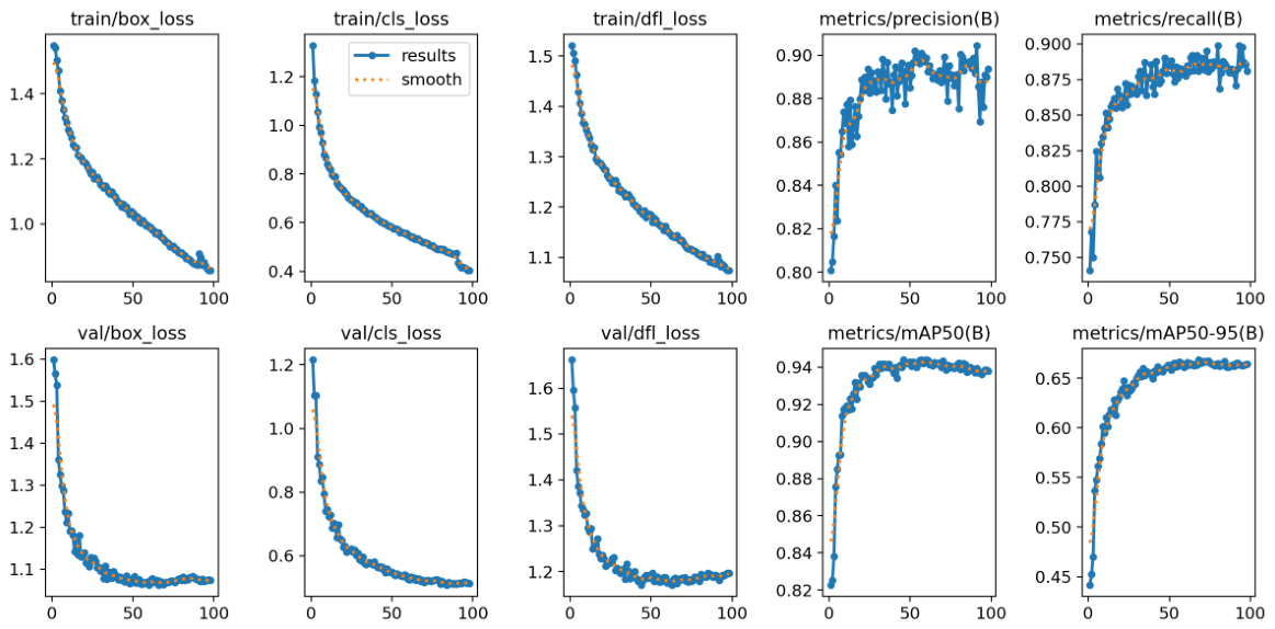
Training of the YOLOv8-based branch detector employed an early-stopping strategy to prevent overfitting. Early stopping was triggered when no improvement was observed for 30 consecutive epochs. The best-performing checkpoint was obtained at Epoch 68 and saved as best.pt, while training terminated at Epoch 98. The total training time was 30.202 h. After stripping the optimizer state, the resulting model size was 22.5 MB.

Figure 5 shows stable convergence of the detector. All training loss components decrease smoothly, while validation losses drop sharply during early epochs and then flatten, indicating that the model learns the main appearance cues quickly and subsequently refines localization. Precision and recall increase rapidly and stabilize around the final operating regime, consistent with the plateau observed in both $\mathrm{mAP}@0.5$ and the stricter mAP@0.5:0.95. Importantly, validation curves track the training trends without divergence, suggesting good generalization and confirming that early stopping is appropriate once mAP saturates. The remaining gap between $\mathrm{mAP}@0.5$ and mAP@0.5:0.95 indicates that further improvements are more likely to come from tighter box regression in difficult cases (e.g., partial occlusion and ambiguous branch boundaries) rather than from additional epochs.

Table 1 summarizes the quantitative detection results on the evaluation set, which contains 461 images and 1990 annotated instances. The detector achieves a precision of 0.893 and a recall of 0.881, corresponding to $\mathrm{mAP}@0.5=0.942$ and mAP@0.5:0.95 = 0.669. These results indicate strong localization accuracy at IoU0.5 and a moderate drop under the stricter COCO-style averaging protocol, as expected in cluttered outdoor scenes with frequent occlusions.

In addition to accuracy, we benchmarked detector runtime under a single standardized on-device protocol on Jetson Orin NX, as described in Section 2.3. Under this protocol, the PyTorch FP32 detector achieved a total latency of 24.4 ms per image (0.4 ms preprocessing, 22.6 ms inference, and 1.4 ms postprocessing), corresponding to approximately 41.0 FPS. Exporting the detector to TensorRT with FP16 precision (best.engine) reduced the total latency to 11.2 ms per image (1.1 ms preprocessing, 7.8 ms inference, and 2.3 ms postprocessing), corresponding to approximately 89.3 FPS, while maintaining comparable detection accuracy. These values are reported under the same consolidated benchmarking protocol and are directly comparable (precision 0.888, recall 0.876, $\mathrm{mAP}@0.5=0.933$, mAP@0.5:0.95 = 0.642). Overall, these results show that TensorRT FP16 provides a strong speed–accuracy trade-off for embedded deployment, with only a small reduction in mAP relative to PyTorch.

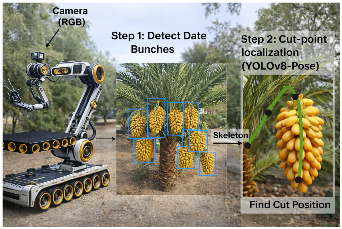
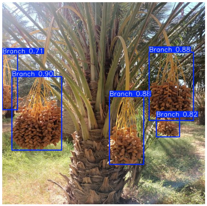
Figure 6 illustrates the detector behavior in a realistic scenario where multiple bunches coexist within the same frame and are surrounded by dense fronds and high-texture background. The model successfully produces multiple consistent detections with high confidence, while also retaining moderate-confidence boxes for partially visible targets. This qualitative evidence supports the quantitative results (high precision/recall and $\mathrm{mAP}@0.5$) and indicates that the detector can handle the multi-target nature of harvesting/pruning scenes, where selecting the best candidate for the second-stage pose estimation may require a top-K strategy or a task-specific ranking criterion (e.g., proximity, visibility, or geometric plausibility).

3.2. Pose (Cut-Point Keypoint Localization)

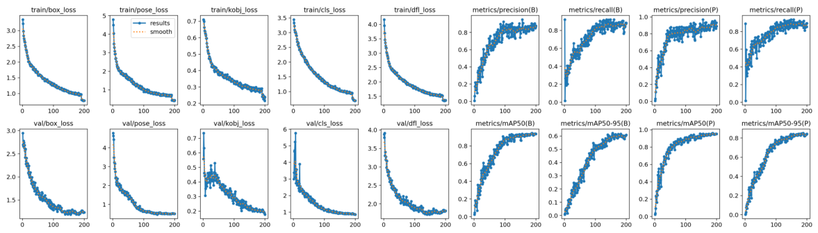
Figure 7 indicates consistent optimization behavior for both detection and keypoint regression. All major loss terms decrease smoothly on the training set, and the validation losses follow the same downward trend, suggesting good generalization and no severe overfitting. The precision and recall for both the box head (B) and the pose head (P) increase rapidly during early epochs and then progressively saturate, which is consistent with the observed plateau in mAP curves (mAP@0.5 and mAP@0.5:0.95). The gradual improvement of the stricter mAP@0.5:0.95 metrics demonstrates that the model continues to refine localization quality beyond coarse alignment, even after mAP@0.5 begins to stabilize.

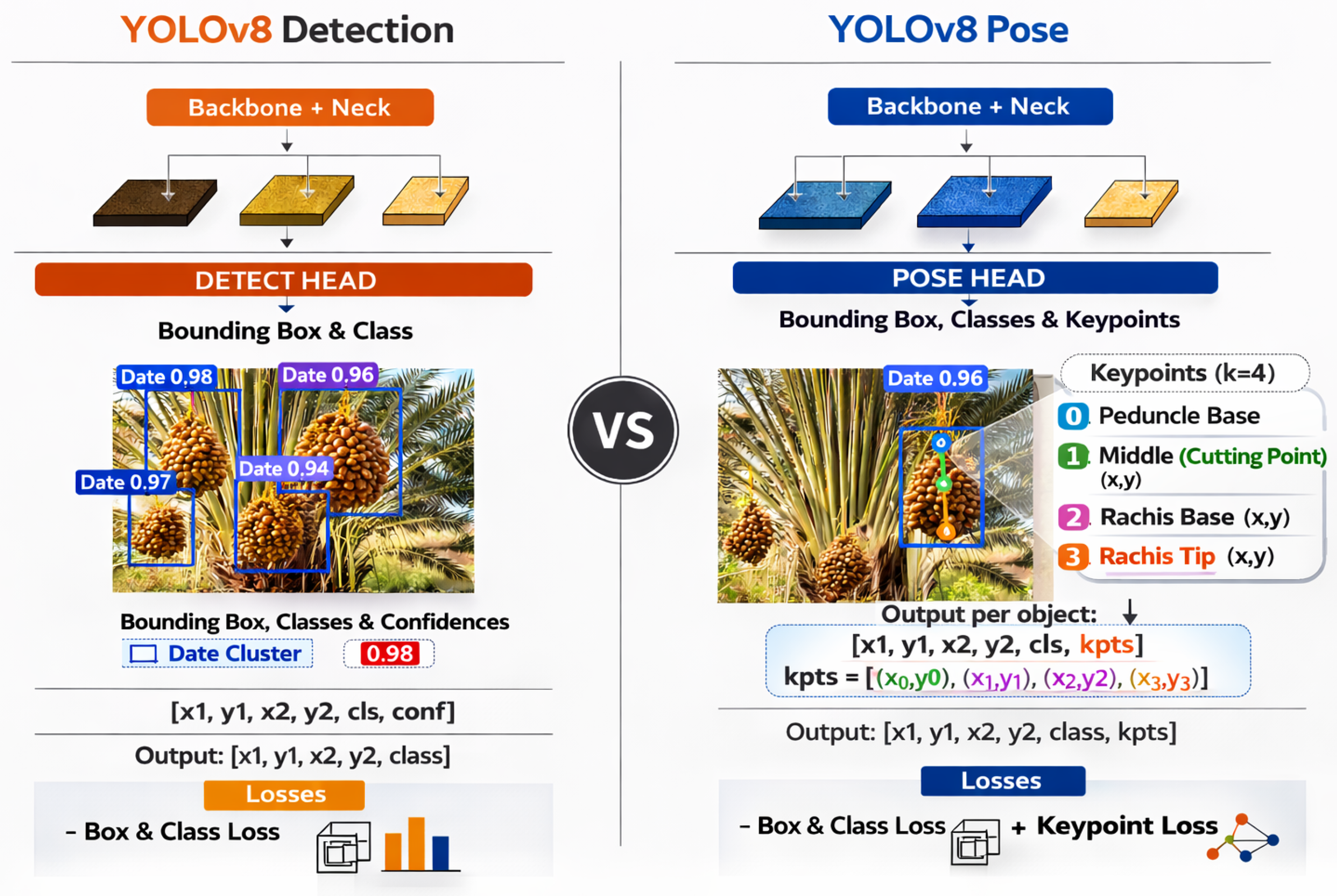
Table 2 reports the performance of the YOLOv8-Pose model for cutting-point localization under two inference backends (PyTorch FP32 and TensorRT FP16). In addition to pose metrics, we also report the internal detection head metrics (Box P/R/mAP) produced by the pose model, since this stage includes both ROI detection and landmark regression.

Under PyTorch (FP32), the model achieves strong pose accuracy with $\mathrm{Pose}P=0.969$ and $\mathrm{Pose}R=0.844$, corresponding to $\mathrm{Pose}\mathrm{mAP}@0.5=0.952$ and PosemAP@0.5:0.95 = 0.840. The associated bounding-box performance is BoxmAP@0.5 = 0.934 and BoxmAP@0.5:0.95 = 0.615 (with $P=0.951$, $R=0.828$). Runtime on the embedded platform is 20.3 ms per image (0.7 ms preprocessing, 13.1 ms inference, 6.5 ms postprocessing), yielding 49.3 FPS.

Exporting the model to TensorRT with FP16 precision accelerates inference while maintaining comparable pose accuracy. TensorRT achieves $\mathrm{Pose}\mathrm{mAP}@0.5=0.953$ and $\mathrm{Pose}\mathrm{mAP}@0.5:0.95=0.824$ with $\mathrm{Pose}P=0.887$ and $\mathrm{Pose}R=0.922$. The box head reports $\mathrm{Box}\mathrm{mAP}@0.5=0.926$ and BoxmAP@0.5:0.95 = 0.601 (with $P=0.854$, $R=0.917$). In terms of latency, TensorRT reduces total runtime to 13.3 ms per image (1.8 ms preprocessing, 5.1 ms inference, 6.4 ms postprocessing), corresponding to 75.2 FPS.

Overall, these results indicate that the pose stage achieves strong within-domain landmark localization performance under the released evaluation split, while a broader robustness characterization across annotation uncertainty, scene subgroups, and explicit correction mechanisms remains outside the scope of the present study.

The pose model achieves consistently high landmark accuracy across both backends, with $\mathrm{Pose}\mathrm{mAP}@0.5\approx 0.95$ and strong $\mathrm{Pose}\mathrm{mAP}@0.5:0.95$ values (0.840 in PyTorch and 0.824 in TensorRT). The small decrease under TensorRT FP16 is expected due to reduced numerical precision, but it remains negligible for practical cutting-point guidance. Interestingly, the backend change alters the precision–recall balance: PyTorch exhibits higher pose precision (0.969) whereas TensorRT increases pose recall (0.922). For harvesting-oriented operation, higher recall is often preferable because missed keypoint predictions translate into missed cutting opportunities; false positives can be mitigated downstream by geometric plausibility checks using the four-keypoint configuration.

Although the pose-stage results are strong under the released evaluation split, they should be interpreted as leakage-controlled within-domain performance rather than as a formal robustness benchmark across systematically stratified occlusion levels, illumination regimes, or cross-oasis acquisition groups. The pose subset remains relatively modest in size (387 images), and the present study does not yet report seed-based confidence intervals or acquisition-group subgroup evaluation across cross-device, cross-session, or cross-oasis variation. However, to provide a more limited robustness characterization within the released split, additional condition-based subgroup analysis for apparent scale, occlusion severity, and illumination difficulty is reported later in Section 3.2.2.

To further examine whether emphasizing individual anatomical landmarks during training improves the task-critical cut-point prediction, we conducted additional single-keypoint weighting ablations centered on direct K1 evaluation (

Table 3. Direct K1 evaluation under the separate matched-prediction ablation protocol for the baseline, K0-weighted, and K1-weighted models.

Model	Split	Count	Mean ${\mathit{E}}_{\mathbf{rel}}$	Median ${\mathit{E}}_{\mathbf{rel}}$	PCK@0.1	PCK@0.2	PCK@0.5
Baseline	Valid	63	0.1227	0.0870	0.556	0.841	0.984
K0-weighted	Valid	64	0.1500	0.1007	0.500	0.797	0.969
K1-weighted	Valid	63	0.1463	0.1078	0.444	0.794	0.968
Baseline	Test	30	0.1388	0.0764	0.600	0.800	0.967
K0-weighted	Test	27	0.1438	0.0839	0.630	0.889	0.889
K1-weighted	Test	26	0.1611	0.1145	0.346	0.808	0.962

Note: These results are reported under a separate direct-K1 matched-prediction ablation protocol for comparative model analysis only. Because the matched prediction sets and counts differ across variants, these values are not directly interchangeable with the primary manuscript metrics reported under the main evaluation protocol.

). Three variants were compared: the baseline model, a K0-weighted variant, and a K1-weighted variant. On the validation split, the baseline provided the strongest overall direct-K1 performance, achieving the lowest relative cut-point error (mean $E_{\mathrm{rel}}=0.1227$, median $=0.0870$) and the highest PCK values (PCK@0.1/0.2/0.5 $=0.556/0.841/0.984$), compared with the K0-weighted model ($0.1500$, $0.1007$, $0.500/0.797/0.969$) and the K1-weighted model ($0.1463$, $0.1078$, $0.444/0.794/0.968$). On the test split, the baseline again achieved the lowest direct-K1 error (mean $E_{\mathrm{rel}}=0.1388$, median $=0.0764$), whereas the K1-weighted model degraded further ($0.1611$, $0.1145$). The K0-weighted model showed higher PCK at $\alpha =0.1$ and $\alpha =0.2$ on its own matched test subset (PCK@0.1/0.2 $=0.630/0.889$), but this occurred with fewer matched predictions (27 vs. 30 for the baseline), higher relative error ($0.1438$ vs. $0.1388$), and lower PCK@0.5 ($0.889$ vs. $0.967$). Overall, under this matched-prediction ablation protocol, the results do not support a consistent benefit from single-keypoint reweighting, and the baseline remains the most consistent direct K1 estimator across the evaluated validation and test conditions.

Latency profiling shows that post-processing is a non-trivial component (6.4–6.5 ms), comparable to or exceeding inference time under TensorRT. This suggests that further speedups may come not only from accelerating the network but also from optimizing the post-processing pipeline (e.g., faster decoding/NMS, batch processing of ROIs, and minimizing CPU–GPU synchronization). Overall, TensorRT FP16 improves throughput from 49.3 to 75.2 FPS (+52%) while maintaining essentially the same pose mAP, making it the recommended backend for embedded deployment of the keypoint stage.

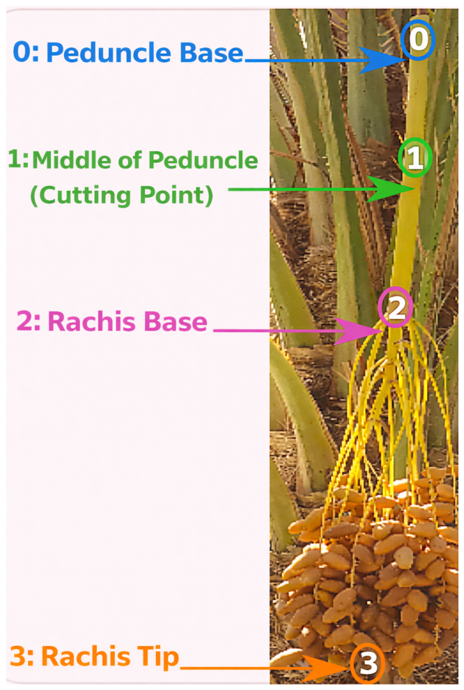
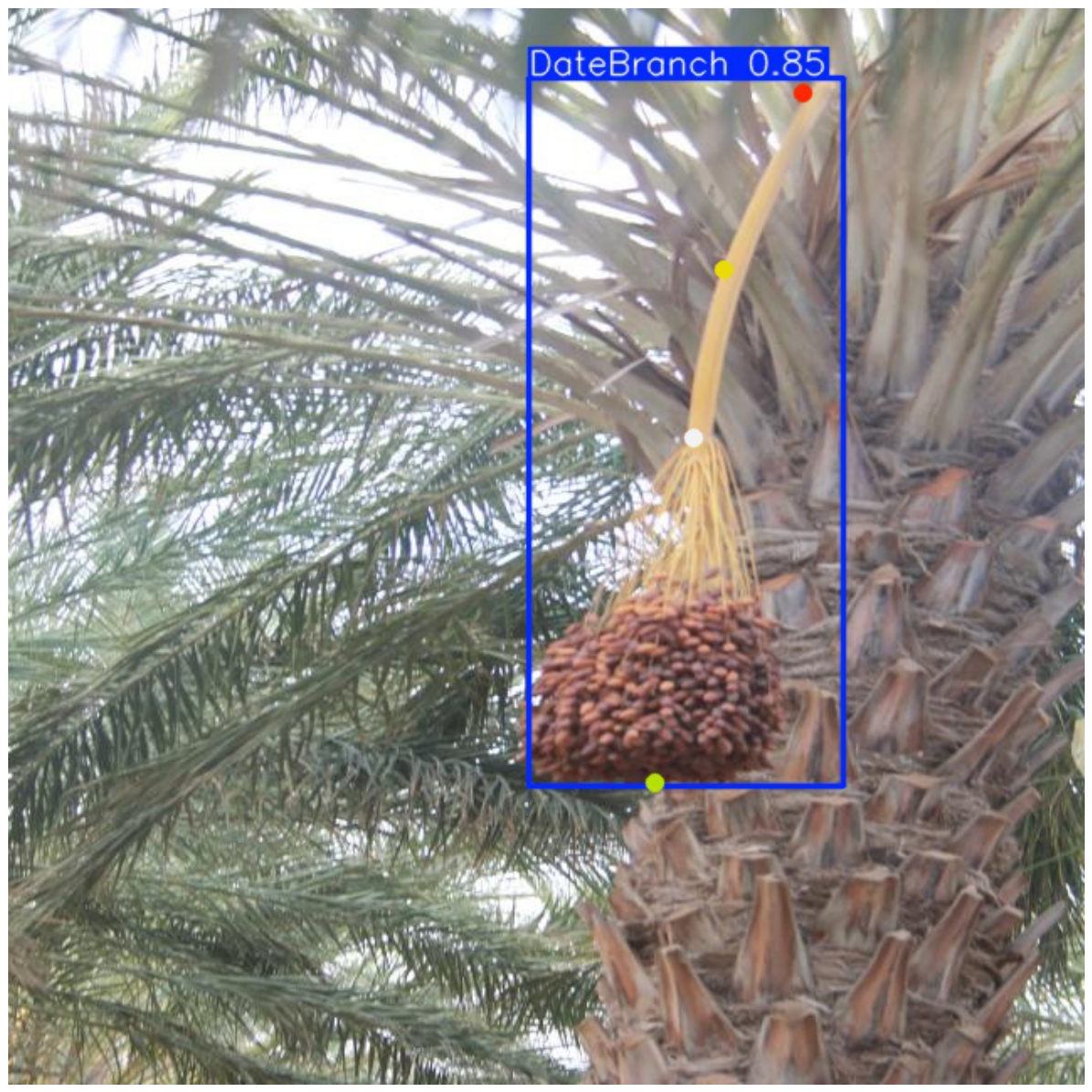
Figure 8 illustrates a representative prediction in a challenging outdoor scene with dense fronds, complex background texture, and non-uniform illumination. Despite the clutter, the detector localizes the target branch with high confidence (0.85), and the pose model places the anatomical landmarks along the branch/peduncle structure in a geometrically consistent configuration. Importantly, the predicted cutting point lies on the peduncle region rather than on the fruit mass, which is consistent with the intended anatomical cutting region. Such examples are consistent with the quantitative results and show that the system can produce anatomically interpretable, task-relevant outputs under challenging within-domain orchard conditions. However, they should not be interpreted as validation of downstream robotic execution or physical cutting performance.

3.2.1. Cut-Point Localization Accuracy (PCK)

To complement mAP-based pose evaluation, we report Percentage of Correct Keypoints (PCK) for the cutting-point landmark under multiple normalized tolerance thresholds $\alpha \in \{0.1,0.2,0.5\}$. PCK measures the fraction of predicted cutting-point keypoints that fall within a distance threshold defined as $\alpha$ times the peduncle reference length

$$L_{\mathrm{ref}}={\parallel K_2-K_0\parallel }_2,$$

where $K_0$ denotes the peduncle base and $K_2$ denotes the rachis base. This reference was chosen because it represents the visible peduncle extent most directly related to the operational cutting point, and is therefore more task-relevant than a generic global scale such as the bounding-box diagonal. Over 256 evaluated cutting-point keypoints, the method achieves $\mathrm{PCK}@\alpha =0.1$ of 0.605 (155/256), $\mathrm{PCK}@\alpha =0.2$ of 0.801 (205/256), and $\mathrm{PCK}@\alpha =0.5$ of 0.871 (223/256) (

Table 4. PCK results for cutting-point localization under different tolerance thresholds.

$\mathit{\alpha }$	Evaluated Keypoints	Correct Keypoints	PCK
0.1	256	155	0.605
0.2	256	205	0.801
0.5	256	223	0.871

). These results indicate that a majority of predictions fall within strict tolerances, and accuracy increases as the tolerance radius relaxes, which is consistent with field conditions where partial occlusions and motion blur can perturb landmark placement.

The PCK analysis provides an image-based interpretation of cut-point localization quality under normalized tolerance thresholds. Under the strict threshold $\alpha =0.1$, approximately 60.5% of predictions are sufficiently close to the ground-truth cut point, reflecting the difficulty of precise landmark placement in cluttered canopy imagery where the peduncle and rachis boundaries may be only partially visible. At $\alpha =0.2$, performance increases to 80.1%, suggesting that many remaining errors are moderate rather than catastrophic. However, no downstream controller, manipulator, or physical cutting validation was performed in the present study. Therefore, these findings should be interpreted strictly as image-based localization results under the reported evaluation protocol, rather than as evidence of execution-level harvesting reliability. In addition, geometric plausibility is not enforced as a hard correction mechanism during inference in the current implementation. The lower gain from $\alpha =0.2$ to $\alpha =0.5$ (0.801 to 0.871) indicates that the remaining failures are not merely small displacements, but correspond to harder cases such as heavy occlusion, ambiguous branch appearance, or incorrect ROI selection.

From a practical standpoint, the strict-threshold result should be interpreted with caution. A PCK@0.1 of 0.605 indicates that the method often localizes the cutting point near the correct peduncle region, but it does not by itself establish that the predicted point is sufficiently precise for autonomous cutting without additional safeguards. The moderate and relaxed thresholds suggest that many errors remain local rather than catastrophic, which is encouraging from a perception perspective; however, the remaining miss rate under the strictest tolerance is still substantial for any deployment scenario that would require direct tool actuation from a single image estimate alone. Accordingly, what has been validated in the present study is image-based cut-point localization under a within-domain evaluation protocol, whereas execution-safe harvesting would require additional steps such as controller integration, geometric or temporal stabilization, metric calibration, and physical cutting trials.

3.2.2. Normalized Cut-Point Accuracy and Tolerance-Based Success

To complement the PCK analysis, we further evaluated the harvest-critical cutting point ($K_1$) using the scale-normalized error defined in the Section 3.2.1. Over all evaluated samples, the normalized cut-point error achieved a median of 0.0866 and a mean of 0.1279. The corresponding tolerance-based success rates were 29.03%, 56.99%, and 73.12% at relative thresholds of 5%, 10%, and 15%, respectively. On the test split, the median normalized error was 0.0764 and the mean was 0.1388, with success rates of 26.67%, 60.00%, and 76.67% at 5%, 10%, and 15% tolerance, respectively.

Table 5. Scale-normalized cut-point error and tolerance-based success rates across dataset splits.

Split	Mean (${\mathit{E}}_{\mathbf{rel}}$)	Median (${\mathit{E}}_{\mathbf{rel}}$)	Success@5%	Success@10%	Success@15%
All	0.1279	0.0866	29.03%	56.99%	73.12%
Valid	0.1227	0.0870	30.16%	55.56%	71.43%
Test	0.1388	0.0764	26.67%	60.00%	76.67%

summarizes the scale-normalized cut-point error and tolerance-based success rates across the validation and test splits, as well as over the full evaluated set.

These results complement strict-tolerance PCK by providing a scale-aware and task-centered view of cut-point localization performance within the studied dataset. They indicate that, while precise localization under the strictest tolerance remains challenging, a substantial proportion of predictions fall within moderate relative error bounds when evaluated with respect to peduncle geometry. This supports the usefulness of the proposed method as an embedded perception module for image-based cut-point localization under the reported within-domain protocol. However, the present results do not by themselves establish physical cutting safety margins, closed-loop controller feasibility, or field-level harvesting reliability, since no downstream execution or physical cutting experiments were conducted.

To further characterize robustness within the released evaluation split, we conducted a subgroup analysis of direct K1 localization with respect to apparent branch scale, occlusion severity, and illumination difficulty. The scale-based results are summarized in

Table 6. Direct K1 subgroup analysis by apparent branch scale under the baseline matched-prediction evaluation protocol.

Scale	Count	Mean ${\mathit{E}}_{\mathbf{rel}}$	Median ${\mathit{E}}_{\mathbf{rel}}$	PCK@0.1	PCK@0.2	PCK@0.5
Small	31	0.2039	0.1598	0.419	0.645	0.935
Medium	31	0.0825	0.0538	0.677	0.903	1.000
Large	31	0.0973	0.0870	0.613	0.935	1.000

Note: These subgroup results are derived from the baseline matched-prediction direct-K1 evaluation subset and are intended to characterize relative robustness trends within the released split, not to replace the primary manuscript metrics reported under the main protocol.

, while the occlusion- and illumination-stratified results are reported in

Table 7. Direct K1 subgroup analysis by occlusion severity and illumination condition under the baseline matched-prediction evaluation protocol.

Factor	Group	Count	Mean ${\mathit{E}}_{\mathbf{rel}}$	Median ${\mathit{E}}_{\mathbf{rel}}$	PCK@0.1	PCK@0.2	PCK@0.5
Occlusion	Low	14	0.0557	0.0657	1.000	1.000	1.000
Occlusion	Moderate	60	0.0928	0.0792	0.617	0.933	1.000
Occlusion	Severe	19	0.2920	0.2676	0.105	0.368	0.895
Illumination	Normal	48	0.0884	0.0625	0.792	0.938	0.979
Illumination	Difficult	45	0.1700	0.1454	0.333	0.711	0.978

Note: These subgroup results are derived from the baseline matched-prediction direct-K1 evaluation subset and are intended to characterize relative robustness trends within the released split, not to replace the primary manuscript metrics reported under the main protocol.

. The scale-based results showed that performance degraded most strongly for the smallest visible branch extent, with mean $E_{\mathrm{rel}}=0.2039$ and PCK@0.1 $=0.419$, compared with $0.0825$ and $0.677$ for the medium-scale group and $0.0973$ and $0.613$ for the large-scale group. This confirms that cut-point localization becomes substantially more difficult when the visible peduncle structure occupies fewer pixels. A similar trend was observed for visibility conditions: severe occlusion produced the weakest performance (mean $E_{\mathrm{rel}}=0.2920$, PCK@0.1 $=0.105$), whereas low-occlusion cases were substantially easier (mean $E_{\mathrm{rel}}=0.0557$, PCK@0.1 $=1.000$). Illumination also had a clear effect, with difficult lighting conditions degrading performance relative to normal illumination (mean $E_{\mathrm{rel}}=0.1700$ vs. $0.0884$; PCK@0.1 $=0.333$ vs. $0.792$). Taken together, these subgroup results indicate that localization reliability remains strongest under medium-to-large apparent scale, low-to-moderate occlusion, and normal illumination, while the principal failure modes are concentrated in small-scale, severely occluded, and difficult-illumination cases.

These subgroup results refine the interpretation of the aggregate normalized-error analysis by showing that the strongest degradation is concentrated in small-scale, severely occluded, and difficult-lighting cases. This further supports the within-domain validity of the proposed perception module while clarifying the main practical conditions under which localization reliability decreases.

A closer reading of these failure patterns suggests that the dominant error modes are not uniform across all samples. In small-scale cases, the visible peduncle structure occupies relatively few pixels, reducing the amount of anatomical detail available to the pose model and making the predicted cut point more sensitive to small localization shifts. Under severe occlusion, the visible peduncle segment may be truncated or partially merged with surrounding fronds, which can distort both landmark ordering and the apparent branch geometry. Difficult illumination introduces a related problem: strong highlights, shadows, or local contrast loss can reduce the visual separability of the peduncle from nearby background structures. In addition, some residual errors are likely attributable not only to landmark regression itself, but also to upstream ROI-selection effects, since the second stage operates on detector-derived crops and may therefore inherit imperfect framing or partial truncation from Stage 1. These observations indicate that the remaining failures are better understood as a combination of visibility limitations, reduced anatomical resolution, and ROI propagation effects, rather than as isolated keypoint-regression noise alone.

A further consideration is annotation uncertainty. Although the four-keypoint protocol was defined using a fixed anatomical convention and the annotations were reviewed iteratively, the present study did not include a formal inter-annotator agreement analysis. This is particularly relevant for the cut-point landmark, since the visible peduncle segment may be partially occluded, weakly contrasted, or only partly exposed in some images, leaving limited visual evidence for an exact point-wise annotation. As a result, part of the residual error near the strictest thresholds may reflect not only model imprecision, but also uncertainty in the target annotation itself. The reported results should therefore be interpreted as performance relative to the current annotation protocol, while a dedicated inter-annotator study remains an important step for future refinement of both the benchmark and the interpretation of fine-grained localization error.

3.2.3. End-to-End Pipeline Latency in Realistic Multi-ROI Scenes

While Table 2 reports the runtime of the pose stage in isolation, practical deployment requires profiling of the complete detect-to-cut pipeline. We therefore additionally measured the end-to-end latency on Jetson Orin NX, including Stage 1 detection, ROI filtering/selection, crop resize preprocessing, Stage 2 pose inference over all selected ROIs, coordinate remapping, and final post-processing (

Table 8. End-to-end latency breakdown of the deployed detect-to-cut pipeline on Jetson Orin NX under realistic multi-ROI scenes.

Scene Type	Avg. ROIs/Frame	Detection (ms)	ROI Select (ms)	Crop/Resize (ms)	Pose Total (ms)	Remap/Post (ms)	Total (ms)	FPS
Single ROI	1	47.27	0.09	3.94	99.48	0.24	151.03	6.65
Two ROIs	2	48.10	0.10	7.79	197.78	0.95	254.72	3.94
Three ROIs	3	187.30	0.11	11.90	532.15	2.72	734.19	2.15
Seven ROIs	7	55.82	0.12	19.83	684.50	1.35	761.62	1.31
Overall	–	83.18	0.10	8.61	287.22	1.24	380.34	4.00

).

Across the evaluated scenes, the complete pipeline achieved a mean total latency of 380.34 ms per frame, with a median of 256.47 ms and a 90th-percentile latency of 582.39 ms. The corresponding mean effective throughput was 4.00 FPS. On average, the latency contribution of each component was 83.18 ms for Stage 1 detection, 0.10 ms for ROI selection, 8.61 ms for crop–resize preprocessing, 287.22 ms for Stage 2 pose inference, and 1.24 ms for coordinate remapping and final post-processing. These results show that the pose stage dominates the end-to-end runtime of the embedded system.

Because Stage 2 is executed sequentially for each selected ROI, the total latency increased with the number of bunch candidates in the scene. Single-ROI scenes required 151.03 ms per frame (6.65 FPS), while two-ROI scenes required 254.72 ms (3.94 FPS). In more crowded scenes, the latency rose to 734.19 ms for three-ROI images (2.15 FPS) and 761.62 ms for a seven-ROI image (1.31 FPS). This behavior provides a more realistic characterization of deployment performance than isolated stage-level timing alone.

This gap between isolated model-stage speed and full pipeline throughput is important for practical interpretation. Although the pose stage alone reaches high throughput under standardized single-image benchmarking, the deployed detect-to-cut system operates under a different constraint regime: Stage 2 must be executed sequentially over the selected ROIs, and the total runtime therefore scales with scene complexity rather than with the nominal FPS of the pose model alone. In practical terms, this means that the reported TensorRT stage-level acceleration should not be interpreted as implying equivalent end-to-end harvesting speed in crowded orchard scenes. Instead, the current system is better understood as a perception prototype whose real-time suitability depends strongly on how many candidate bunches are forwarded to the second stage. This distinction is especially important because the pipeline remains substantially more feasible in sparse or single-target scenarios than in multi-ROI scenes with high target density.

In the deployed implementation, Stage 2 is executed sequentially for each selected ROI; therefore, the total frame latency depends directly on the number of bunch candidates present in the scene. These results should be interpreted cautiously in terms of practical harvesting feasibility. While the isolated detector and pose-stage benchmarks indicate that both modules can run efficiently on Jetson Orin NX, the complete deployed pipeline is substantially slower in realistic multi-ROI scenes because Stage 2 is executed sequentially for each selected region. In particular, the mean end-to-end throughput of 4.00 FPS, together with the drop to 3.94 FPS for two-ROI scenes and 2.15 FPS for three-ROI scenes, suggests that the current implementation is better viewed as an embedded perception prototype than as a fully deployment-ready harvesting solution for crowded orchard conditions. From a practical perspective, these results support onboard feasibility for perception-guided branch analysis, but they also indicate that additional system-level optimization will be necessary before claiming robust real-time operation in multi-target harvesting scenarios.

3.2.4. Video-Based Runtime and Temporal Stability

To further assess deployment behavior beyond still-image inference, we evaluated the complete pipeline on a continuous video sequence captured under a single-bunch scenario. Over 448 processed frames, the system selected one ROI in 445 frames and no ROI in only 3 frames, indicating stable target acquisition throughout the sequence. As summarized in

Table 9. Video-based runtime and temporal stability of the deployed detect-to-cut pipeline on Jetson Orin NX under a single-bunch scenario.

Metric	Mean	Median
Detection latency (ms)	36.27	33.72
Crop/Resize latency (ms)	4.94	5.19
Pose latency (ms)	93.70	93.01
Total latency (ms)	135.01	131.69
Effective FPS	7.79	7.59
Raw $k_1$ displacement (px)	111.11	57.65
Smoothed $k_1$ displacement (px)	39.96	24.99

, the complete pipeline achieved a mean total latency of 135.01 ms per frame (median 131.69 ms), corresponding to an average effective throughput of 7.79 FPS. The mean latency contributions were 36.27 ms for Stage 1 detection, 4.94 ms for crop–resize preprocessing, and 93.70 ms for Stage 2 pose inference, again confirming that the pose stage dominated the runtime.

We additionally examined the temporal stability of the harvest-critical cutting point $k_1$ across consecutive frames. Without temporal filtering, the frame-to-frame displacement of the predicted cut point had a mean of 111.11 px and a median of 57.65 px. After applying exponential moving average smoothing, these values decreased to 39.96 px and 24.99 px, respectively, corresponding to an approximate reduction of 64.0% in the mean displacement and 56.6% in the median displacement. This indicates that lightweight temporal smoothing can substantially reduce frame-to-frame fluctuation of the predicted cut point in video deployment. Since the evaluated sequence was not frame-wise annotated, these results should be interpreted as temporal stability indicators rather than absolute localization accuracy.

During sustained locked-clock execution on Jetson Orin NX, the system exhibited stable operating behavior, with an average power draw of 10.28 W, a peak power draw of 14.82 W, an average peak-per-sample temperature of 61.66 °C, a peak temperature of 66.22 °C, and no observed thermal throttling. To complement the runtime analysis with a basic embedded-systems characterization, we monitored power and thermal telemetry using tegrastats during sustained execution under the locked-clock 25 W Jetson Orin NX configuration described in Section 2.3.

Table 10. Power and thermal behavior during sustained embedded execution on Jetson Orin NX under the locked-clock 25 W configuration.

Scenario	Avg. Power (W)	Peak Power (W)	Avg. Temp. (°C)	Peak Temp. (°C)	Throttling
Sustained deployed run	10.28	14.82	61.66	66.22	No

reports the average power draw, peak power draw, average peak-per-sample temperature, peak temperature, and whether thermal throttling was observed during the monitored run. These values provide an operational indication of sustained deployment behavior beyond latency alone.

4. Comparison Study

To position our contribution within the recent literature,

Table 11. Comparison with related work on embedded YOLO-based perception and harvesting oriented localization.

Work	Application/Task	Model/Approach	Hardware (Edge)	Output	Performance	Notes
Ariaux et al. [6] (2025)	Timber screwing: target pose	YOLOv8 seg. + pose	Jetson AGX Orin	Seg./pose	Acc. 94.6%; ∼50 ms/frame	Real-time edge pose for robotic action.
De Guia & Deveraj [7] (2025)	AV: det. + pose + tracking	Unified YOLOv8 multi-task	Jetson AGX Orin	BBoxes + 17 kpts + tracks	∼20 Hz; ∼50 ms; $640\times 640$	Integrated multi-task perception.
Karacaoglu & Sahin [8] (2025)	Kiwi detection (occlusion)	YOLOv8–YOLOv11 benchmark	Jetson TX2	BBoxes	mAP@0.5 ≈ 0.956; ∼0.3 FPS	Accuracy/latency trade-offs on TX2.
You et al. [9] (2025)	Apple detection (weather)	Pruned YOLOv8n	Jetson Orin Nano	BBoxes	mAP50 89.0%; 102.6 FPS	Compression enables high-speed detection.
Du et al. [10] (2025)	Pomegranate monitoring	YOLOv8n + DPDM/CCFM	Embedded (n/r)	BBoxes	mAP 92.6%; ∼14.3 FPS	Task-specific lightweight design.
Lin et al. [11] (2025)	Peach detection (occlusion)	YOLOv11n + attention/AMFP	Embedded (n/r)	BBoxes	mAP@0.5:0.95 ≈ 62.7%	Robustness under occlusion.
Teng et al. [14] (2023)	Vineyard pruning targets	Faster R-CNN + Mask R-CNN	n/r	Regions/masks	Up to 0.97 detection rate	Pruning perception (not embedded-focused).
Liang et al. [15] (2025)	Tomato pruning points	YOLOv5 + geometric cut rule	n/r	Masks + cut-point	n/r	Actionable cut-point coordinates.
Wang et al. [16] (2025)	Pepper cut-point localization	YOLO + clustering + geometry	n/r	Det. + cut-point	∼28 FPS; ∼20 mm error	Learned det. + geometry hybrid.
Maji et al. [20] (2022)	Joint det. + 2D pose	YOLO-Pose (OKS loss)	n/r	BBoxes + kpts	AP50∼90.2	One-stage detection + keypoints.
Periyasamy et al. [21] (2023)	Robotics 6D pose	YOLOPose V2 (transformer)	n/r	6D pose/kpts	Real-time (n/r)	End-to-end pose for robotics.
This work	Two-stage branch detection and cut-point localization	YOLOv8-m + YOLOv8-Pose (4 kpts)	Jetson Orin NX	Boxes + 4 kpts + cut-point	Det. mAP@0.5 0.942; Pose mAP@0.5 0.952; Stage-level TRT FP16: 89/75 FPS; End-to-end: 4.00 FPS overall, 7.79 FPS single-bunch video	PCK@$\alpha =0.1/0.2/0.5$: 0.605/0.801/0.871.

Note: Reported values are reproduced from the cited works; differences in datasets, evaluation protocols, and hardware configurations should be considered when interpreting cross-study comparisons.

summarizes representative works that employ YOLO-based perception on embedded/edge hardware and/or produce action-oriented outputs such as keypoints, poses, or cut-point estimates for robotic manipulation and harvesting. Overall, prior studies follow two dominant directions: (i) improving detection robustness in challenging agricultural scenes (occlusion, clutter, and variable illumination), and (ii) accelerating inference through model compression and deployment optimizations (e.g., TensorRT) to achieve real-time performance on resource-constrained platforms. However, many embedded-oriented works remain limited to bounding-box detection without converting perception outputs into an operational decision (e.g, a cutting point), while several localization approaches report limited on-device runtime characterization. In this context, our system combines fast Stage 1 Branch/DateBranch detection with Stage 2 keypoint-based cut-point localization tailored to harvesting, and reports both accuracy and end-to-end latency on a Jetson Orin NX platform.

Compared with prior embedded agricultural perception studies, the main strength of the present work is not merely detector-level speed or landmark regression in isolation, but the integration of a two-stage detect-to-cut pipeline that produces an anatomically meaningful cutting point and reports both embedded stage-level timing and realistic end-to-end deployed latency. At the same time, the comparison also highlights several limitations. Relative to detector-oriented embedded studies, our end-to-end throughput is substantially more constrained in crowded multi-ROI scenes because the second stage is executed sequentially over the selected ROIs. Relative to systems that combine learned perception with explicit geometric decision rules, the present implementation remains more conservative, since geometric plausibility is used only as an interpretation framework and not yet as an activated correction layer. Moreover, while the proposed system advances beyond coarse object detection by producing a task-relevant cut point, it is still evaluated as an image-based perception module rather than as a fully validated harvesting controller.

Accordingly, the evidence established in this study should be interpreted in a balanced way. What has been validated is that, under a leakage-controlled within-domain evaluation protocol, the proposed embedded pipeline can localize candidate bunches, estimate harvest-relevant landmarks, produce a task-centered cut-point prediction, and operate onboard Jetson Orin NX with clearly quantified runtime trade-offs. What has not yet been validated is execution-level harvesting feasibility, cross-group generalization across oases, sessions, or devices, or the practical benefit of activating geometry-based correction within the deployed inference loop. These aspects remain important next steps and motivate future work on controller integration, physical cutting trials, group-aware robustness evaluation, and system-level optimization for multi-ROI operation.

5. Conclusions

This paper presented a two-stage embedded detect-to-cut perception prototype for date palm branch analysis, combining YOLOv8-based branch detection with YOLOv8-Pose keypoint localization to infer an anatomically meaningful cutting point. Quantitative evaluation shows that the detector achieves high performance ($P=0.893$, $R=0.881$, $\mathrm{mAP}@0.5=0.942$, mAP@0.5:0.95 = 0.669), while the pose model provides accurate landmark estimation (Pose $\mathrm{mAP}@0.5\approx 0.95$) and reliable cut-point localization measured by PCK (0.605 at $\alpha =0.1$, 0.801 at $\alpha =0.2$, and 0.871 at $\alpha =0.5$). Embedded benchmarking on Jetson Orin NX demonstrates the feasibility of leakage-controlled within-domain on-device perception for the studied setting. However, the reported results should be interpreted as evidence for an embedded perception prototype under the released evaluation protocol, not as validation of a field-ready harvesting system or of cross-domain generalization across oases, sessions, cultivars, or deployment conditions.

A natural extension of the present work is to incorporate geometric plausibility more explicitly, either as a soft regularization term during training or as a lightweight post-prediction consistency filter during inference.

From a deployment perspective, the current system should be interpreted as a practical FP16 embedded realization rather than a full compression study. Future work will therefore examine whether additional optimization strategies, such as pruning, INT8 quantization, distillation, or adaptive selective computation, can further improve the balance among cut-point accuracy, latency, and power consumption on embedded agricultural platforms.

Future work will also include detector-scale ablations (e.g., YOLOv8-n/s/m) and systematic analysis of ROI crop resolution and padding, particularly for the pose stage, where cut-point localization is sensitive to the spatial representation of the peduncle region.