Application of Machine Learning Methods for Predicting Susceptibility to Lung Cancer and Identifying Predictors Influencing the Risk of Lung Cancer Development

Abstract

Lung cancer is still one of the major contributors to cancer-related mortality. Treatment effectiveness depends directly on early diagnosis and accurate prediction of disease progression. This study focuses on the application of classical machine learning algorithms —including Logistic Regression, Support Vector Machine, Random Forest, and XGBoost —for questionnaire-based lung cancer risk assessment. A comparative study of six machine learning algorithms used to predict lung cancer based on survey data was conducted. According to the ROC-AUC metric, Random Forest model achieved the best result. In terms of F1-score and precision for the positive class, the support vector machine (SVM) demonstrated the highest efficiency. However, gradient boosting provided the most balanced results across key clinical metrics. SHAP (SHapley Additive exPlanations) analysis identified three preliminary predictors potentially associated with lung cancer risk in this sample: seeing a pulmonologist, unexplained weight loss, and loss of appetite. These preliminary results are consistent with clinical observations and suggest the potential interpretability of ensemble machine learning approaches in medical diagnostics, though confirmation on larger datasets is required. Overall, the preliminary results suggest the potential of using machine learning methods for lung cancer screening based on questionnaire data, particularly with an expanded training sample. Potential applications of early lung cancer diagnosis are discussed. Further research in this area will be conducted in conjunction with image recognition of computed tomography scans.

1. Introduction

The increase in cancer incidence is one of the most relevant problems in the modern world. Early diagnosis of lung cancer significantly increases patient survival. The application of artificial intelligence in this field represents a promising direction for further development. While deep learning methods have shown promise in automating image analysis, classical machine learning approaches offer practical advantages for questionnaire-based screening due to their interpretability and lower data requirements.

According to the World Health Organization [1], lung cancer is the leading cause of cancer mortality worldwide, with approximately 2.5 million new cases and 1.8 million deaths were registered in 2022. The study by Cao M. et al. [2] presents current data on the global burden of lung cancer from the GLOBOCAN 2022 database, as well as long-term incidence projections through 2050. Mikubo M. et al. [3] found that the five-year survival rate for lung cancer does not exceed 25% and remains critically low due primarily to late detection of the disease. This underscores the high medical and social significance of developing early diagnostic tools.

The work of Hosseini M.S. et al. [4] presents a systematic review of lung cancer diagnostic methods based on computed tomography, conducted prior to the advent of deep learning techniques, including radiography, bronchoscopy, and biopsy. Alzubaidi M.A. et al. [5] showed that interpreting CT scans using traditional methods largely depends on the specialist’s qualifications and incurs significant time costs. The study by Zhan X. et al. [6] developed an intelligent medical system based on CNNs to support clinical decision-making in the diagnosis of non-small cell lung cancer, opening a new direction for integrating neural networks into medical decision-making systems.

At the same time, traditional approaches have several significant limitations. Shen D. et al. [7] found that deep learning algorithms require significant computational resources and large labeled datasets, which substantially limit their application in routine clinical practice. In their work, Obermeyer Z. and Emanuel E.J. [8] showed that traditional clinical decision-making models are significantly inferior to machine learning methods in processing large volumes of unstructured medical data. Callender T. et al. [9] reported that expert systems based on predefined rules are unable to adapt to new patterns without manual updates to the knowledge base.

The study by Dritsas E. and Trigka M. Reference [10] compared machine learning algorithms for lung cancer prediction and demonstrated the high robustness of ensemble methods to class imbalance. Li Y. et al. [11], in a review of machine learning methods in oncological diagnostics, showed that ML algorithms can automatically extract informative features from multidimensional clinical datasets and model nonlinear dependencies that are inaccessible to traditional statistical methods. Oentoro J. et al. [12], in a systematic review of machine learning implementations for lung cancer prediction, confirmed that ensemble and hybrid approaches demonstrate the most consistent results on imbalanced medical datasets. Alsinglawi B. et al. [13] developed an interpretable framework based on the SHAP method and the Random Forest algorithm, with SMOTE-based class balancing, achieving an AUC of 98%, thereby confirming the promise of explainable models in clinical diagnostics.

The work of Faruqui N. et al. [14] proposed a hybrid model, LungNet, that combines deep convolutional neural networks with medical IoT data for lung cancer diagnosis, achieving 96.8% accuracy. Alsheikhy A.A. et al. [15] developed an automated diagnostic system based on a hybrid VGG-19 and LSTM architecture for early lung cancer detection from CT scans, achieving over 98.8% accuracy. Ali A. et al. [16], in a review of deep learning methods for lung cancer diagnosis, showed that integrating CNNs with transformers and multimodal data achieves the highest accuracy for malignant neoplasm classification. In a systematic review, Zahid A.B. et al. analyzed 70 studies published from 2014 to 2025 on deep and hybrid learning for lung nodule detection and classification. At the same time, most of the reviewed works focus on image analysis, whereas screening models based on clinical questionnaires remain understudied [17].

At the same time, as established by Pan Z. et al. [18], predictive models based on questionnaire data and clinical predictors, applicable at the preclinical screening stage, remain insufficiently studied despite their practical availability.

Similar to the work of Yang R. et al. [19], which applied RF, XGBoost, and SHAP to predict EGFR mutations in lung cancer, the present study conducted a comparative analysis of six ML algorithms with SHAP interpretation, while also developing an expert system for early lung cancer diagnosis based on clinical predictors. Callender T. et al. [20] demonstrated the effectiveness of machine learning applied to real-world clinical data for lung cancer risk prediction, emphasizing the importance of model validation on independent population samples.

Su M.C. proposed using neural networks as medical diagnosis expert systems, demonstrating how trained networks can extract knowledge in the form of production rules applicable to clinical diagnostics [21]. The work of Lisboa P.J.G. et al. presented a systematic review of the application of ANNs in oncological diagnostics and decision support [22]. Cruz J.A. et al. reviewed ML models for cancer prediction and diagnosis and described additional possible applications of these methods [23].

In the studies by Kourou K. et al., practical examples of the use of artificial intelligence in oncological diagnostics were provided [24]. Karabatak M. et al. proposed a hybrid system combining rules with a neural network [25]. Polat K. et al. compared intelligent methods for cancer diagnosis [26].

Akay M.F. et al. proposed using patient symptom features for early cancer diagnosis [27]. Abbass H.A. proposed an evolutionary artificial neural network approach based on Pareto-differential evolution for breast cancer diagnosis [28]. Ahmed F.E. reviewed the application of ANNs for diagnosis and survival prediction in colon cancer, demonstrating the advantages of neural networks over traditional statistical methods in oncological prognosis [29].

Delen D. et al. proposed using clinical tabular patient data as predictors for a neural network model for cancer prediction [30].

In the work of Street W.N. et al., the Wisconsin Breast Cancer dataset—a classic benchmark in the field—was proposed for early breast cancer diagnosis [31]. Yan Y. et al. reviewed the development and use of CNNs for tumor diagnosis [32].

Keles A. et al. proposed an expert system based on neuro-fuzzy rules for breast cancer diagnosis, demonstrating the effectiveness of interpretable rule-based neural systems in oncological diagnostics [33]. Jang J.S.R. et al. proposed a basic architecture of neuro-fuzzy systems for early diagnosis of oncological diseases [34]. Setiono R. et al. proposed rule extraction from a trained network to improve cancer diagnosis accuracy [35].

In the studies of Kononenko I. et al., the use of structured symptoms and patient responses for disease diagnosis is proposed [36]. Lavrač N. et al. proposed a diagnosis based on questionnaires and medical databases using neural networks [37].

Podgorelec V. et al. proposed a rule-based question-answering system for clinical systems [38]. Bibault J.E. et al. proposed the use of AI in personalized oncology [39]. In their work of Esteva A. et al. reviewed the use of AI in medical diagnostics [40]. In studies by Topol E.J. et al., prospects for implementing AI in healthcare were proposed [41].

Elinor Nemlander et al. used an adaptive electronic questionnaire, the PEX-LC, in which patients answered questions about symptoms, feelings, and risk factors. Machine learning algorithms were then applied to predict lung cancer in never smokers, former smokers, and current smokers. The results showed the model’s good predictive ability and the importance of stratifying patients by smoking status [42].

In the work by Songjing Chen et al., large-scale web-based questionnaires were administered to elderly patients. A deep neural network identified hidden risk factors for the development of lung cancer. The study confirmed that neural networks can identify nonlinear relationships between questionnaire parameters that are difficult to detect with classical statistics [43].

The literature review confirms the high relevance of developing an expert system for early cancer diagnosis based on question-and-answer interactions using neural networks. This approach is particularly promising for lung, breast, stomach, and colorectal cancers, where early detection significantly increases survival.

Despite the growing body of research on machine learning for lung cancer prediction, most existing studies rely on CT imaging data, which requires expensive equipment and specialist interpretation. Questionnaire-based screening models applicable at the preclinical stage remain understudied. Furthermore, few studies combine multiple ML algorithms with SHAP-based interpretability analysis on survey data. The present study addresses this gap by developing and comparing six machine learning models for lung cancer risk prediction based on a clinical questionnaire, and using SHAP analysis for feature interpretation and threshold optimization to improve model evaluation.

2. Materials and Methods

This study aims to develop and evaluate machine learning models to predict lung cancer risk from patient questionnaire data. To prepare the inputs for the cancer prediction model, a questionnaire was created with questions on lung cancer diagnosis, based on the protocol ‘Lung Cancer—Clinical Protocols of the Ministry of Health of the Republic of Kazakhstan, dated 1 July 2022, Protocol No. 164.’ A total of 219 respondents completed the questionnaire. All participants provided informed consent, and the questionnaire was anonymous, since the processed data does not include respondents’ names and surnames. Approval from the ethics committee was obtained.

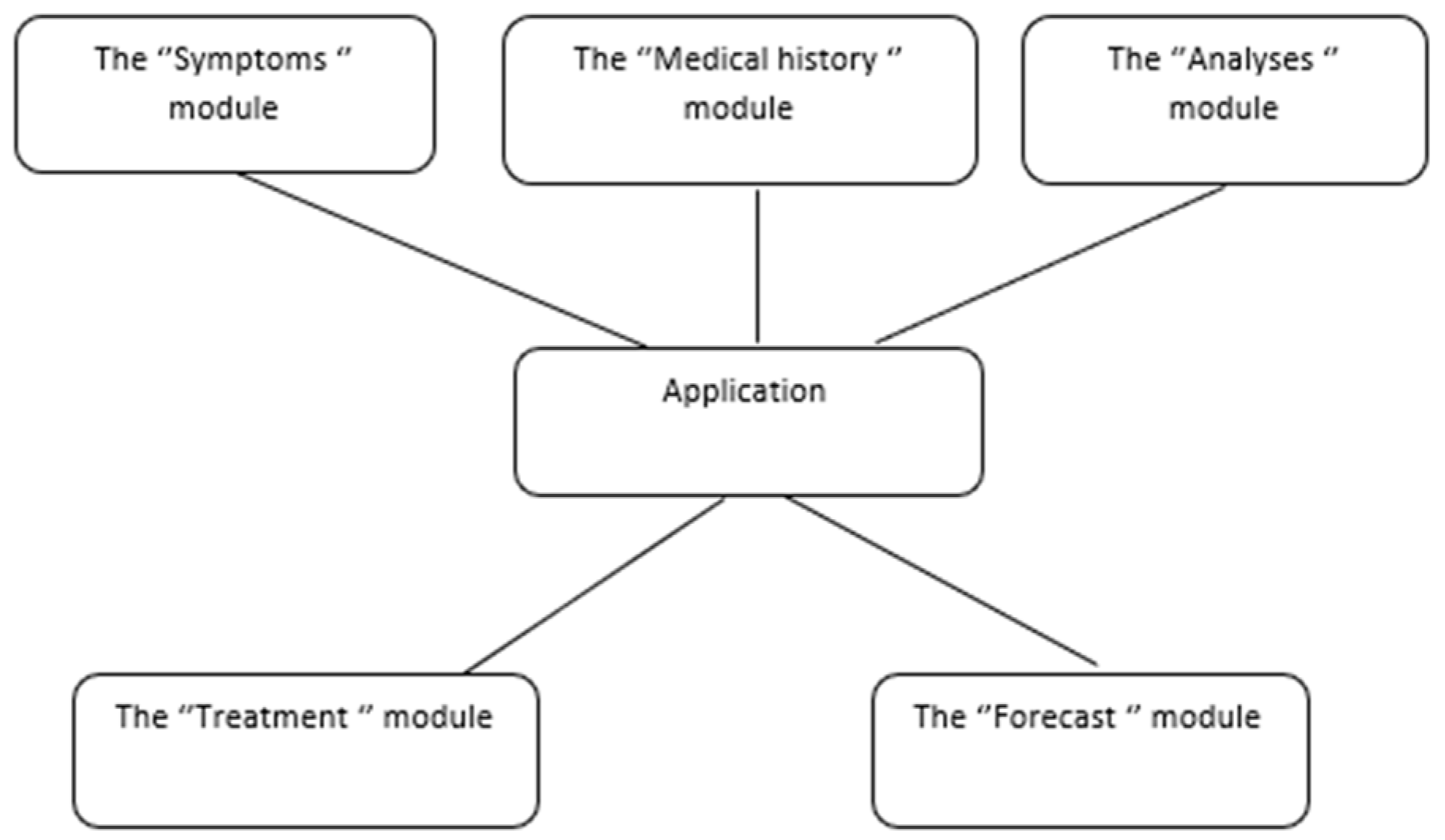
To create an early lung cancer diagnosis system, it is necessary to define the system structure, including the main modules and their functions. The following system structure is proposed, consisting of the interconnected modules shown in Figure 1. The system consists of the following modules: Symptoms, Medical Histories, Tests, Application, Treatment, and Prognosis.

The “Symptoms” module stores information about symptoms of various lung diseases, including oncological diseases.

The “Medical Histories” module contains information about patients’ medical histories, whether confirmed and unconfirmed.

The “Tests” module manages data from instrumental and clinical studies conducted on patients.

The “Application” module processes the survey results.

The “Treatment” module stores information about treatment protocols for various lung diseases.

The “Prognosis” module calculates the probability of a patient’s susceptibility to lung cancer [44,45].

After determining the system structure, it is necessary to define the stages of system construction. The following stages are proposed:

• Definition of rules and facts of the expert system for lung cancer diagnosis based on the knowledge of oncologists;
• Identification of the lung cancer risk group;
• Determination of lung cancer probability using the application;
• Referral of patients at high risk of lung cancer susceptibility to a physician.

As a result of studying the subject area with oncologists, the main predictors for the knowledge base were identified: age, sex, smoking duration, frequency of viral infections, family cancer history, presence of a dry cough, and weight loss. Each rule has between 1 and 5 answers, the values of which range from 0 to 1, depending on the specific weight of the answer to the question. The classification of key diagnostic aspects is illustrated in

Table 1. Rules and facts of the expert system.

No	Question/Rule
1	Age
2	sex
3	Do you smoke?
4	Smoking duration
5	How many times a year do you get acute respiratory viral infections (ARVI)
6	Family cancer history (parents and close relatives)
7	Have you ever had hemoptysis?
8	Do you experience shortness of breath or a feeling of lack of air?
9	Do you experience unexplained weakness?
10	Have you been coughing?
11	Have you had any difficulty swallowing?
12	Have you had any chest pain?
13	Have you had any pain in your arm or shoulders?
14	Have you had a dry cough?
15	Have you had any unexplained weight loss?
16	Have you had any loss of appetite?
17	Are you under medical follow-up “D” registration with a pulmonologist for other lung diseases?

.

These rules and facts were used in the neural network’s expert system to model the system’s reasoning logic.

Stage 2. Identifying the lung cancer risk group

Based on the rules and facts of the subject area, a questionnaire for early lung cancer diagnosis was compiled. More than 200 people completed the questionnaire.

Description of the dataset

The initial data for modeling were collected through the questionnaire survey. The questionnaire covers 21 features reflecting demographic characteristics, risk factors, and clinical symptoms associated with lung cancer. Three records were excluded from the analysis due to missing values in the target variable. The final sample consisted of 216 observations. The target variable takes two values: 0—lung cancer not detected, 1—lung cancer detected.

The class distribution is characterized by a pronounced imbalance: 208 observations (96.3%) belong to class 0, and 8 observations (3.7%) belong to class 1. This ratio is typical of medical datasets where disease cases occur significantly less frequently than their absence. The main characteristics of the dataset are shown in

Table 2. Characteristics of the original dataset.

Characteristics	Value
Initial number of records	219
Number of records after filtering	216
Number of input features	21
Target variable	Presence of lung cancer (0/1)
Class 0—cancer not detected	208 (96.3%)
Class 1—cancer detected	8 (3.7%)
Class ratio	26:1
Missing values imputation: “Smoking duration”	Median imputation 6 observations
Missing values imputation: “Packs of cigarettes per day”	Excluded due to 71.3% missing values

.

The feature ‘Packs of cigarettes per day’ was excluded from the final analysis due to 71.3% missing values (n = 154), as imputation of such a high proportion would introduce substantial bias and reduce model reliability. The remaining missing values in ‘Smoking duration’ (n = 6) were imputed using median imputation, which is robust to outliers commonly present in medical data.

Datasplitting

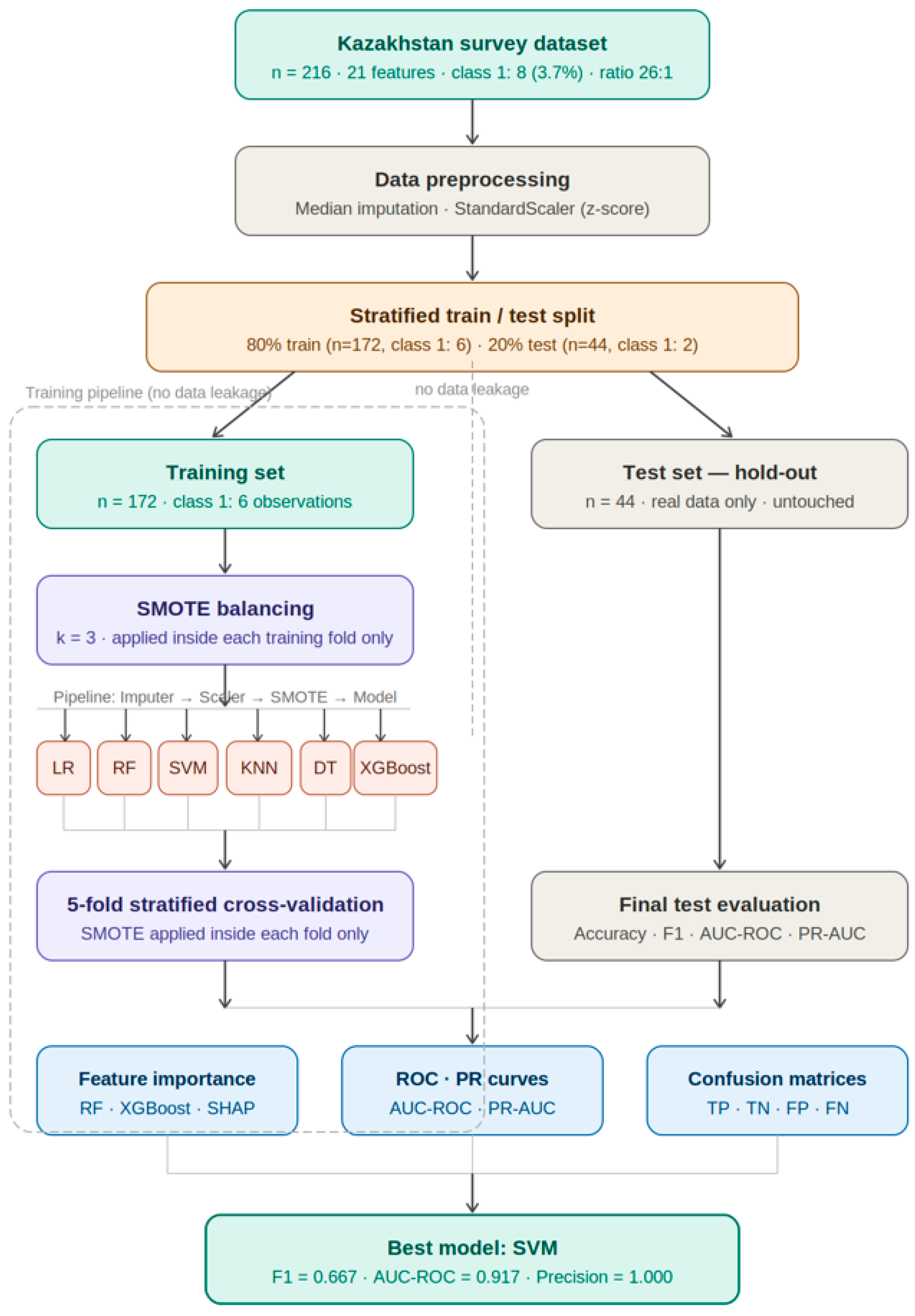
Before processing, the dataset was split into training (80%, n = 172) and testing (20%, n = 44) sets, while preserving the class ratio in each set (stratification). The test set contains 2 lung cancer patients and 42 non-cancer patients. This test set is completely isolated and does not participate in preprocessing, balancing, or model training, which ensures an independent and objective assessment of the models’ ability to generalize to new data. The overall research scheme is shown in Figure 2 and consists of the following steps: Data preprocessing, Training, Class balancing using SMOTE, Model interpretation, and Analysis.

Data Preprocessing

Preprocessing is performed strictly within the training set. Missing values in the “Smoking duration” feature are filled using the median imputation method. The median was chosen as a measure of central tendency because it is robust to outliers, which are characteristic of medical data. After missing-value imputation, all features are standardized using a z-score transformation, resulting in each feature having a zero mean and unit standard deviation. This process is necessary for the correct operation of algorithms sensitive to data scale, particularly support vector machines and logistic regression. When testing the model, the preprocessing parameters calculated exclusively on the training set are applied to the test set.

Class balancing using the SMOTE method

To address class imbalance, the SMOTE (Synthetic Minority Over-sampling Technique) method is applied.

SMOTE generates synthetic observations of the minority class by linear interpolation between existing observations and their nearest neighbors in the feature space. The number-of-neighbors parameter is set to k = 3 because the training set contains only 6 positive observations. The use of the standard value k = 5 is excluded because it is technically impossible to apply it given this data volume.

SMOTE must be applied exclusively to the training set within a single data processing pipeline. The test set contains only real observations, with no synthetic data. This approach prevents data leakage—a methodological error in which information from the test set is indirectly used for model training, leading to artificially inflated quality metrics.

Data processing pipeline

For proper experimental organization, all preprocessing and balancing steps are combined into a single pipeline that sequentially includes: median imputation for missing values, feature standardization, and SMOTE balancing. The pipeline is trained only on the training data of each split and applied to the validation data without any modifications. This ensures that the validation and test data do not influence the preprocessing and balancing parameters, which is a mandatory condition for obtaining reliable estimates of model quality.

Stage 3. Determination of lung cancer probability using the application

This study compares six machine learning algorithms, including linear, nonlinear, and ensemble approaches, for binary classification.

Logistic regression (LR) estimates the probability of an observation belonging to class 1 based on a linear combination of features using the sigmoid function. The model is used as a baseline for comparison.

The support vector machine (SVM) constructs a separating hyperplane that maximizes the margin between classes. In this work, a radial basis function (RBF) kernel is used to model nonlinear class boundaries.

K-nearest neighbors (KNN) classifies a new observation into the class that predominates among k = 5 nearest neighbors in the training set.

Decision tree (DT) builds a hierarchical structure of classification rules by recursively partitioning the feature space. The maximum tree depth is limited to five levels to avoid overfitting.

Random forest (RF) is an ensemble of 100 decision trees, each trained on a random subsample of data and features. The final prediction is determined by averaging the trees’ predictions.

XGBoost implements gradient boosting, in which trees are built sequentially, and each subsequent tree corrects the errors of the previous one.

The hyperparameter settings for all machine learning models used in this study are summarized in

Table 3. Hyperparameter settings for all machine learning models.

Model	Hyperparameter	Value
Logistic Regression (LR)	Regularization (C)	1.0
Logistic Regression (LR)	Solver	lbfgs
Logistic Regression (LR)	Max iterations	1000
Support Vector Machine (SVM)	Kernel	RBF
Support Vector Machine (SVM)	Regularization (C)	1.0
Support Vector Machine (SVM)	Gamma	scale
K-Nearest Neighbors (KNN)	Number of neighbors (k)	5
K-Nearest Neighbors (KNN)	Distance metric	Euclidean
Decision Tree (DT)	Max depth	5
Decision Tree (DT)	Criterion	Gini
Random Forest (RF)	Number of trees	100
Random Forest (RF)	Max features	sqrt
Random Forest (RF)	Random state	42
XGBoost	Learning rate (η)	0.1
XGBoost	Max depth	6
XGBoost	Number of estimators	100
XGBoost	Random state	42

. All models were trained using default or commonly recommended parameter values, with the exception of SMOTE, where the number of neighbors was reduced to k = 3 due to the limited number of positive training samples.

Quality assessment metrics

Six metrics are used to evaluate model quality, and their definitions are given in

Table 4. Classification quality assessment metrics.

Metric	Formula	Value in Medical Diagnostics
Accuracy	(TP + TN)/(TP + TN + FP + FN)	Overall proportion of correct classifications
Precision	TP/(TP + FP)	Proportion of correct predictions among those predicted as positive
Recall	TP/(TP + FN)	Proportion of detected real cancer cases
F1-Score	2 × P × R/(P + R)	Balance between Precision and Recall
AUC-ROC	Area under the ROC curve	Ability of the model to rank patients by risk
PR-AUC	Area under the PR curve	Quality of minority class detection

. In medical diagnostic tasks, Recall and F1-Score are priority metrics since missing a real case of lung cancer (false negative, FN) entails significantly more serious clinical consequences than erroneously classifying a healthy patient as at risk (false positive, FP).

Additionally, PR-AUC (area under the Precision–Recall curve) is calculated, which is a more informative metric than ROC-AUC in cases of severe class imbalance, as it does not account for true negatives and focuses directly on the quality of minority-class detection.

Validation scheme

Model robustness is assessed using stratified five-fold cross-validation on the training set. Stratification ensures that the original class ratio is preserved in each split. At each step, the preprocessing and balancing pipeline is reapplied exclusively to the training part of the current split, while the validation part remains untouched. After cross-validation is completed, each model is retrained on the entire training set and finally tested on the held-out test set.

Feature importance analysis

To identify clinically significant predictors of lung cancer, feature importance is analyzed using two algorithms: Random Forest and XGBoost. In Random Forest, feature importance is determined as the average reduction in the Gini index from splits on that feature across all trees in the ensemble. In XGBoost, feature importance is calculated as the total improvement in the objective function when the feature is used during boosting. Consistency between the two algorithms’ results increases the reliability of conclusions about the predictive significance of features.

Confusion matrix analysis

The confusion matrix is used for a detailed analysis of each model’s predictions. It allows the evaluation of four metrics: true negatives (TN)—healthy patients correctly identified as healthy; false positives (FP)—healthy patients erroneously classified as at risk; false negatives (FN)—cancer patients missed by the model; true positives (TP)—cancer patients correctly identified by the model. In oncological diagnostics, the FN metric has the greatest clinical significance.

Feature correlation analysis

Correlation analysis is performed to assess linear relationships among input features using the Pearson correlation coefficient. Pairs of features with a correlation coefficient above 0.8 are considered potential sources of multicollinearity, which reduces the interpretability of linear models. The analysis was performed on the original dataset before balancing.

Patient profile analysis

To identify clinical differences between patient groups, a comparative analysis of mean feature values is performed. For each feature, the difference in mean values between the “cancer detected” group (n = 8) and the “cancer not detected” group (n = 208) is calculated. Features with the largest difference are considered the most significant clinical indicators of the disease.

Model interpretation using SHAP

The SHAP (Shapley Additive exPlanations) method is used to interpret model predictions. The SHAP value of each feature indicates how much, and in what direction, it changes the predicted probability of cancer for a particular patient relative to the model’s average prediction. The TreeExplainer, which provides accurate calculations for tree-based ensemble methods, is used to compute SHAP values. The results are presented in three visualization forms: SHAP Feature Importance, SHAP Summary Plot, and SHAP Waterfall Plot for an individual patient from the test set.

3. Results

Before testing on an independent set, a preliminary assessment of the model’s robustness is conducted. The training set is split into five equal parts. The model is alternately trained on four parts and validated on the fifth. The procedure is repeated five times to ensure that each part is used exactly once for validation. At each step, class balancing using SMOTE is applied exclusively to the training data, while the validation part remains untouched. This eliminates data leakage and ensures an objective assessment of the model quality.

The results are presented in

Table 5. Results of five-fold cross-validation on the training set.

Model	F1 in Each Fold	Mean F1 ± Range	Mean AUC ± Range
LR	[0.0, 0.0, 0.0, 0.0, 0.4]	0.080 ± 0.160	0.384 ± 0.364
RF	[0.0, 0.0, 0.0, 0.0, 0.0]	0.000 ± 0.000	0.828 ± 0.235
SVM	[0.0, 0.0, 0.0, 0.0, 0.667]	0.133 ± 0.267	0.737 ± 0.200
KNN	[0.333, 0.0, 0.0, 0.286, 0.286]	0.181 ± 0.149	0.843 ± 0.190
DT	[0.0, 0.0, 0.0, 0.0, 0.0]	0.000 ± 0.000	0.488 ± 0.006
XGBoost	[0.0, 0.0, 0.0, 0.0, 0.0]	0.000 ± 0.000	0.776 ± 0.321

. The F1-Score values vary significantly from one split to another. In most cases, the models do not detect any lung cancer cases (F1 = 0). Only in certain splits are acceptable values achieved: SVM—to 0.667; KNN—to 0.333. The average F1-Score across all splits does not exceed 0.181 for any model. Meanwhile, AUC-ROC values remain relatively high for Random Forest (0.828) and KNN (0.843), indicating that these models can rank patients by risk level even when the standard classification threshold does not detect positive cases.

The instability of the F1-Score is primarily explained by the extremely small number of positive cases in the training set: when split into five parts, each training group contains only 4–5 lung cancer patients. Under such conditions, even a small change in the data composition significantly affects the result. Thus, cross-validation confirms that with such a small number of positive cases, none of the studied algorithms provides stable detection of the minority class. The results confirm that the main limitation is not the choice of algorithm but the insufficient data volume.

The final assessment of model quality is conducted on a held-out test set comprising 20% of the original data (n = 44), which includes 2 lung cancer patients and 42 non-cancer patients. The test set was not used at any stage of training or data balancing. Each model is trained using a unified preprocessing pipeline (imputation, scaling, SMOTE). The results are presented in

Table 6. Classification results on the test set (n = 44).

Model	Accuracy	Precision	Recall	F1-Score	AUC-ROC	PR-AUC
LR	0.9318	0.3333	0.5000	0.4000	0.4762	0.1894
RF	0.9318	0.0000	0.0000	0.0000	0.9762	0.5833
SVM	0.9773	1.0000	0.5000	0.6667	0.9167	0.6111
KNN	0.8636	0.2500	1.0000	0.4000	0.9762	0.6667
DT	0.9318	0.3333	0.5000	0.4000	0.7262	0.1894
XGBoost	0.9318	0.0000	0.0000	0.0000	0.8929	0.3500

.

To address the zero Recall of Random Forest and XGBoost at the standard threshold, classification threshold optimization was performed for all models. Threshold optimization was performed as a post hoc exploratory analysis on the test set due to the limited sample size, and the results should be interpreted as exploratory rather than definitive. The results are presented in

Table 7. Classification results on the test set with optimized classification threshold (n = 44).

Model	Optimal Threshold	Accuracy	Precision	Recall	F1-Score	AUC-ROC	PR-AUC
LR	0.49	0.9318	0.3333	0.5000	0.3333	0.4762	0.1894
RF	0.30	0.9318	0.6667	1.0000	0.8000	0.9762	0.5833
SVM	0.24	0.9773	1.0000	0.5000	0.6667	0.9167	0.6111
KNN	0.80	0.9773	1.0000	0.5000	0.6667	0.9762	0.6667
DT	0.05	0.9318	0.5000	0.5000	0.5000	0.7262	0.1894
XGBoost	0.15	0.9318	0.5000	0.5000	0.5000	0.8929	0.3500

.

Threshold optimization significantly improved the performance of Random Forest and XGBoost models. Random Forest achieved the best overall result with an optimal threshold of 0.30, yielding an F1-Score = 0.800 and a Recall = 1.000, thereby successfully identifying all lung cancer cases in the test set with only one false positive. XGBoost improved from an F1 = 0.000 to F1 = 0.500 with a threshold of 0.15. These results confirm that the standard 0.5 classification threshold is unsuitable for tasks with severe class imbalance and that threshold optimization is mandatory in medical diagnostic applications.

SVM achieved an F1-Score (0.667) without yielding any false-positive predictions among healthy patients (Precision = 1.000). This means that all patients classified by the SVM model as having cancer truly belong to the positive class. Although the model identifies only one of the two real lung cancer patients, it still demonstrates the best balance between sensitivity and precision among the considered algorithms. This result suggests the potential usefulness of SVM in tasks with limited medical data.

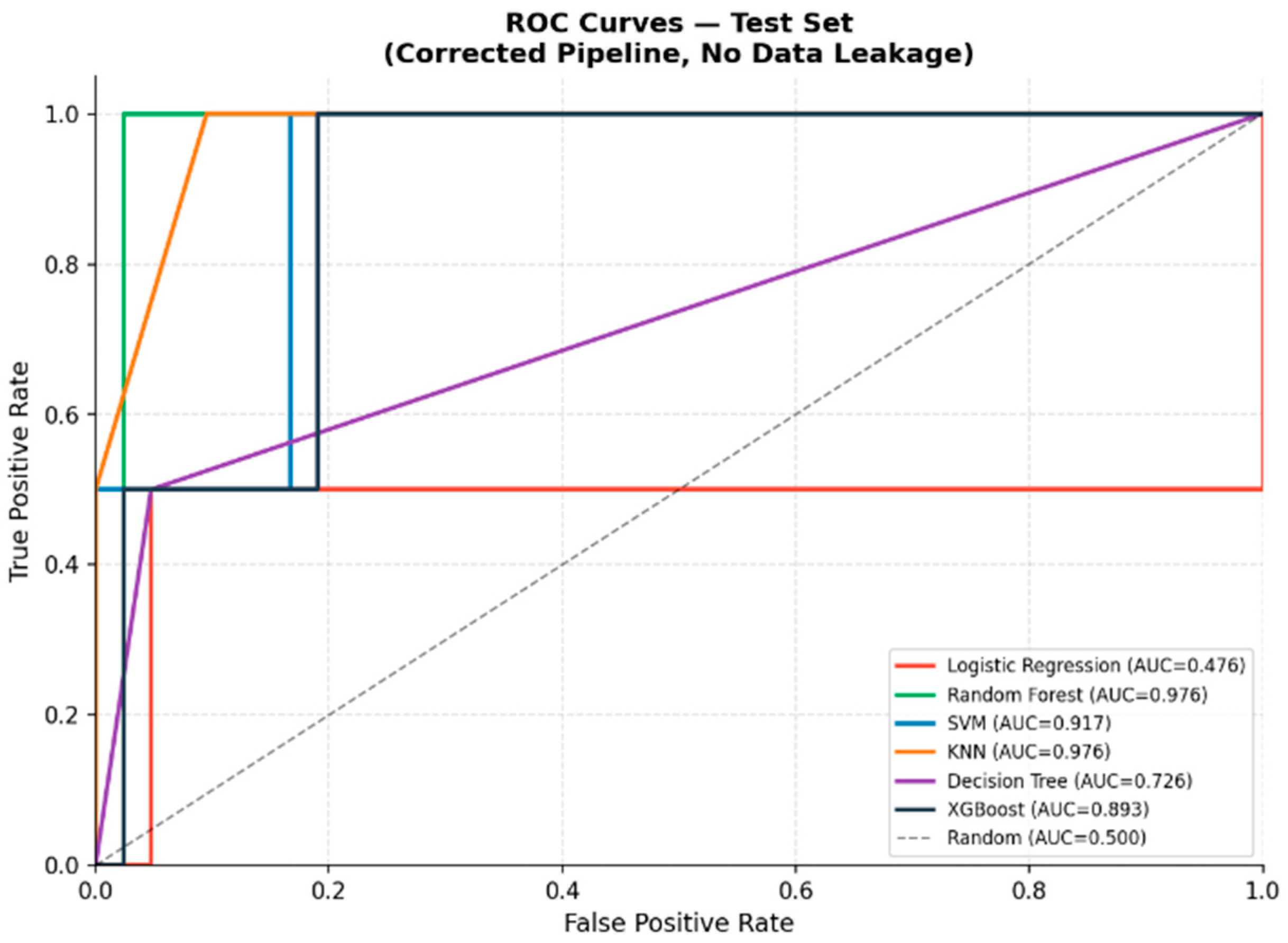
KNN detects both lung cancer patients (Recall = 1.000), but erroneously classifies six healthy patients as at risk. This indicates high model sensitivity and low specificity, which is typical for distance-based algorithms with small sample sizes. Random Forest and KNN show the best AUC-ROC value of 0.976. Random Forest and XGBoost do not detect any cancer cases at the standard classification threshold, despite their high AUC-ROC values. This indicates that these models require individual tuning of decision thresholds for tasks with severe class imbalance. The high ROC-AUC values with zero Recall for several models indicate a mismatch between the standard classification threshold and tasks with severe class imbalance. Under these conditions, classification threshold optimization becomes critically important.

ROC curves and Precision–Recall curves. The ROC curves are presented in Figure 3. The ROC curves show how well the models distinguish between patients with and without cancer at different classification thresholds. The closer the curve is to the top-left corner, the better the model. Random Forest and KNN (AUC = 0.976) are located closest to the ideal value, while Logistic Regression (AUC = 0.476) shows a result worse than random guessing.

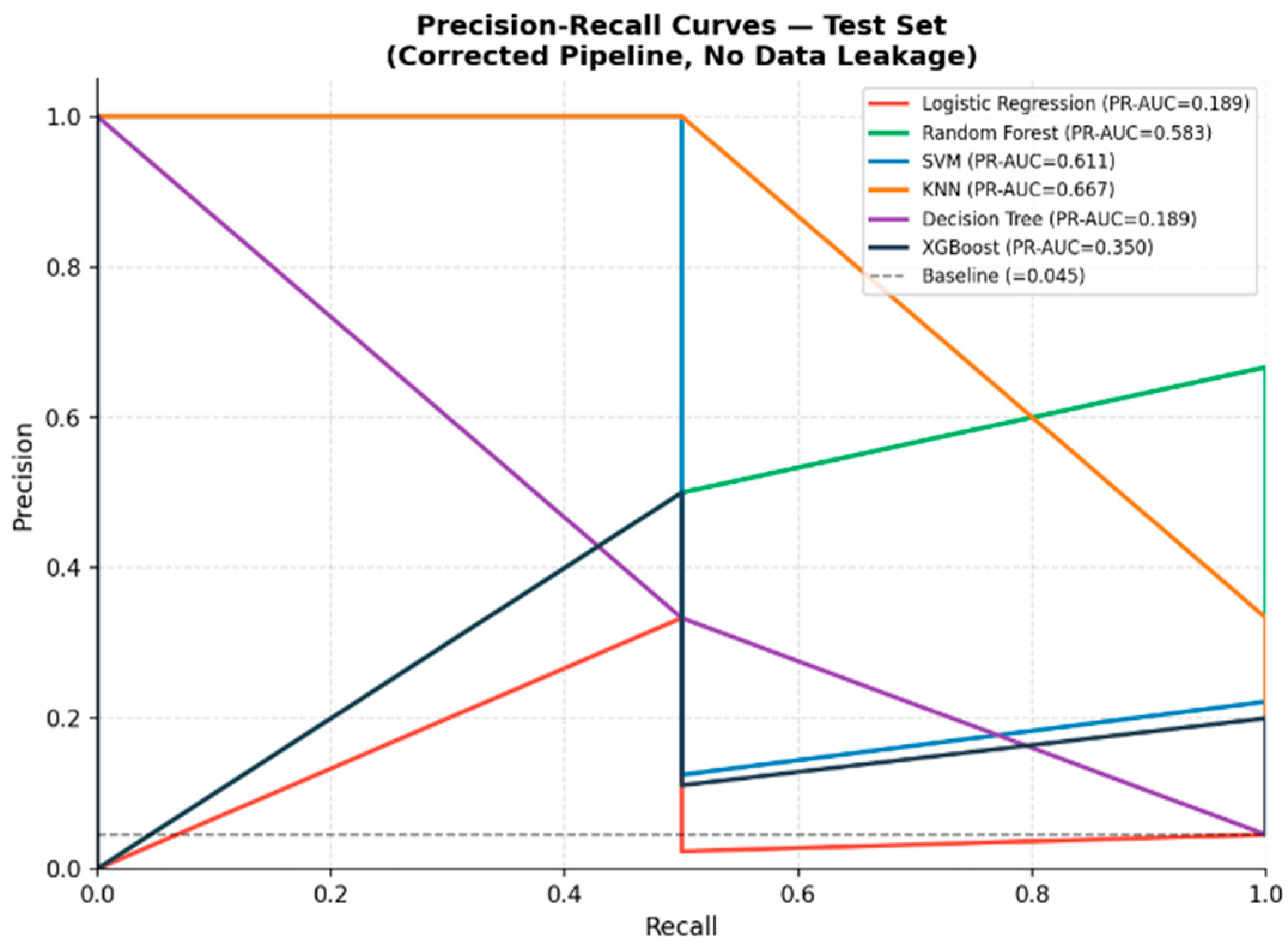
The Precision–Recall curve provides a more informative metric in cases of severe class imbalance, as it focuses directly on the quality of positive class detection. Unlike the ROC-AUC, PR-AUC more accurately reflects model quality in the presence of a rare positive class. Precision–Recall curves are presented in Figure 4. KNN achieves the best PR-AUC of 0.667, followed by SVM at 0.611. The baseline for a random classifier is 0.045, which corresponds to the proportion of cancer patients in the test set. All models except LR and DT significantly exceed this level.

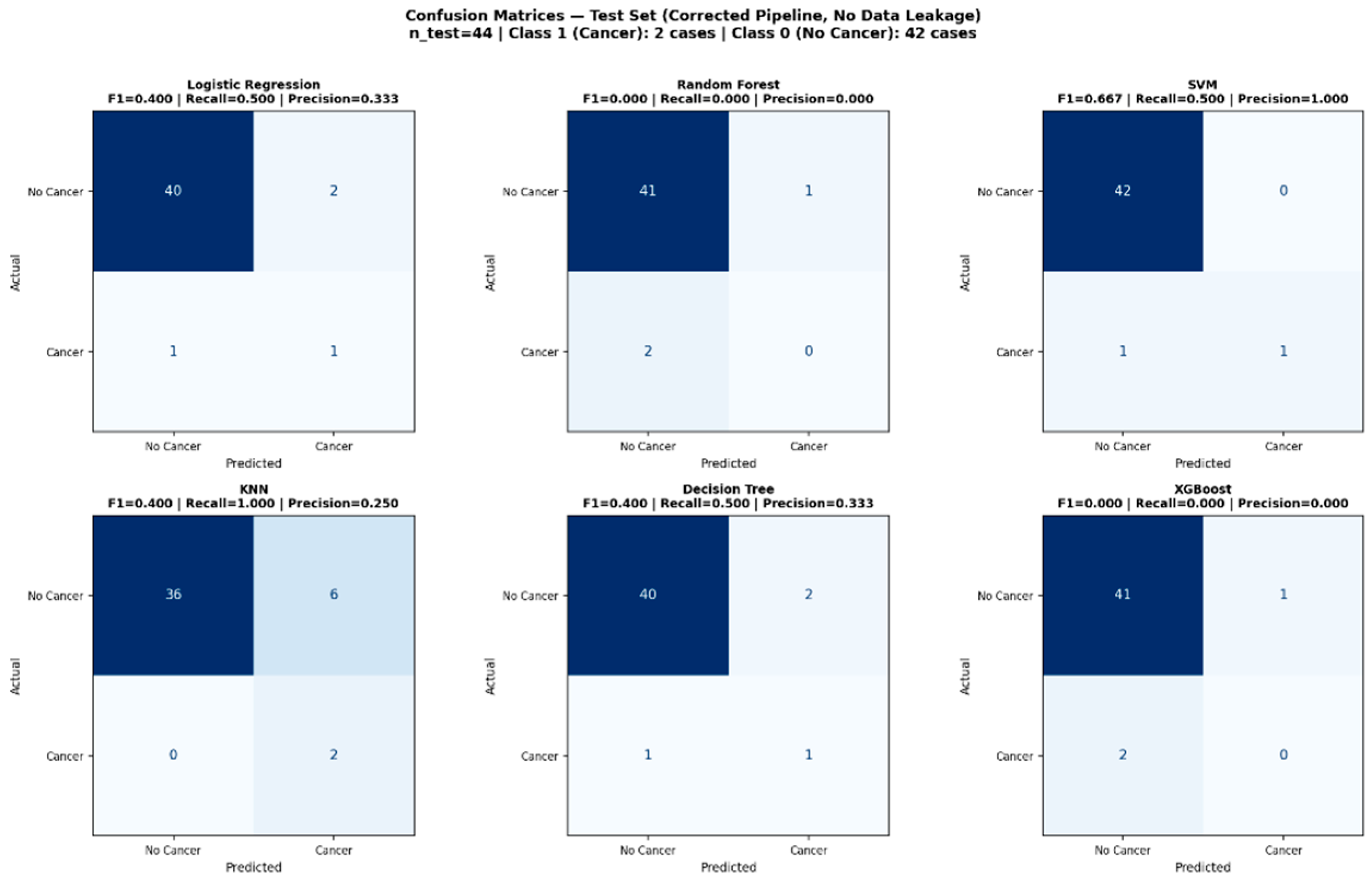
The confusion matrix shows how many patients the model classified correctly and how many incorrectly. It contains four metrics: true negatives (TN)—healthy patients correctly identified as healthy; false positives (FP)—healthy patients erroneously classified as at risk; false negatives (FN)—cancer patients missed by the model; true positives (TP)—cancer patients correctly identified by the model. Confusion matrices for all six models are presented in Figure 5. In medical diagnostics, the FN metric has the greatest clinical significance because missing a real cancer case delays treatment initiation and worsens prognosis. Model results for this metric differ significantly. SVM: TN =42, FP = 0, FN = 1, TP = 1—the only model without false positive predictions. KNN: TN = 36, FP = 6, FN = 0, TP = 2—the only model without missed cancer cases. LR, DT: TN = 40, FP = 2, FN = 1, TP = 1—intermediate result. RF, XGBoost: TN = 41–42, FP = 0–1, FN = 2, TP = 0—both real cancer cases were missed.

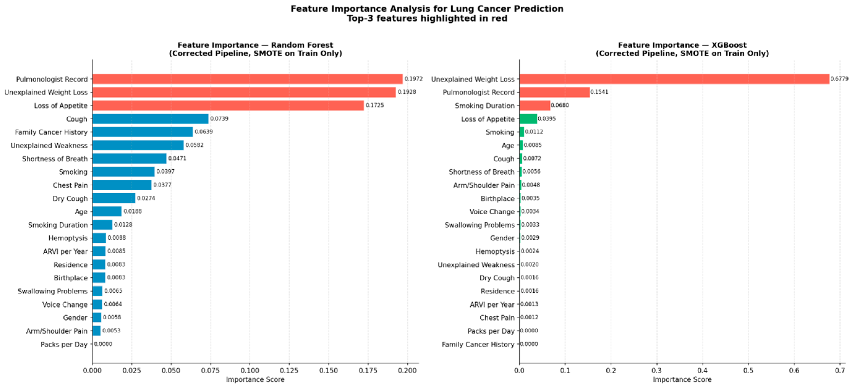
The results of the feature importance analysis are presented in Figure 6. The top three most significant features are highlighted in red. Both algorithms, Random Forest and XGBoost, consistently identify three features as the most significant predictors of lung cancer. “Unexplained weight loss” ranks first according to XGBoost (0.678) and second according to Random Forest (0.193).”Pulmonologist follow-up for lung diseases” ranks first according to Random Forest (0.197) and second according to XGBoost (0.154). “Loss of appetite” is in the third position according to Random Forest (0.173). These symptoms correspond to the clinical presentation of lung cancer and are consistent with the results of previous studies.

SHAP analysis allows us to explain why a model makes a particular prediction for each patient. Unlike general feature importance, SHAP shows both the magnitude and the direction of each feature’s influence: whether it increases or decreases the predicted probability of cancer for a specific patient. The results are presented in Figure 7, Figure 8 and Figure 9.

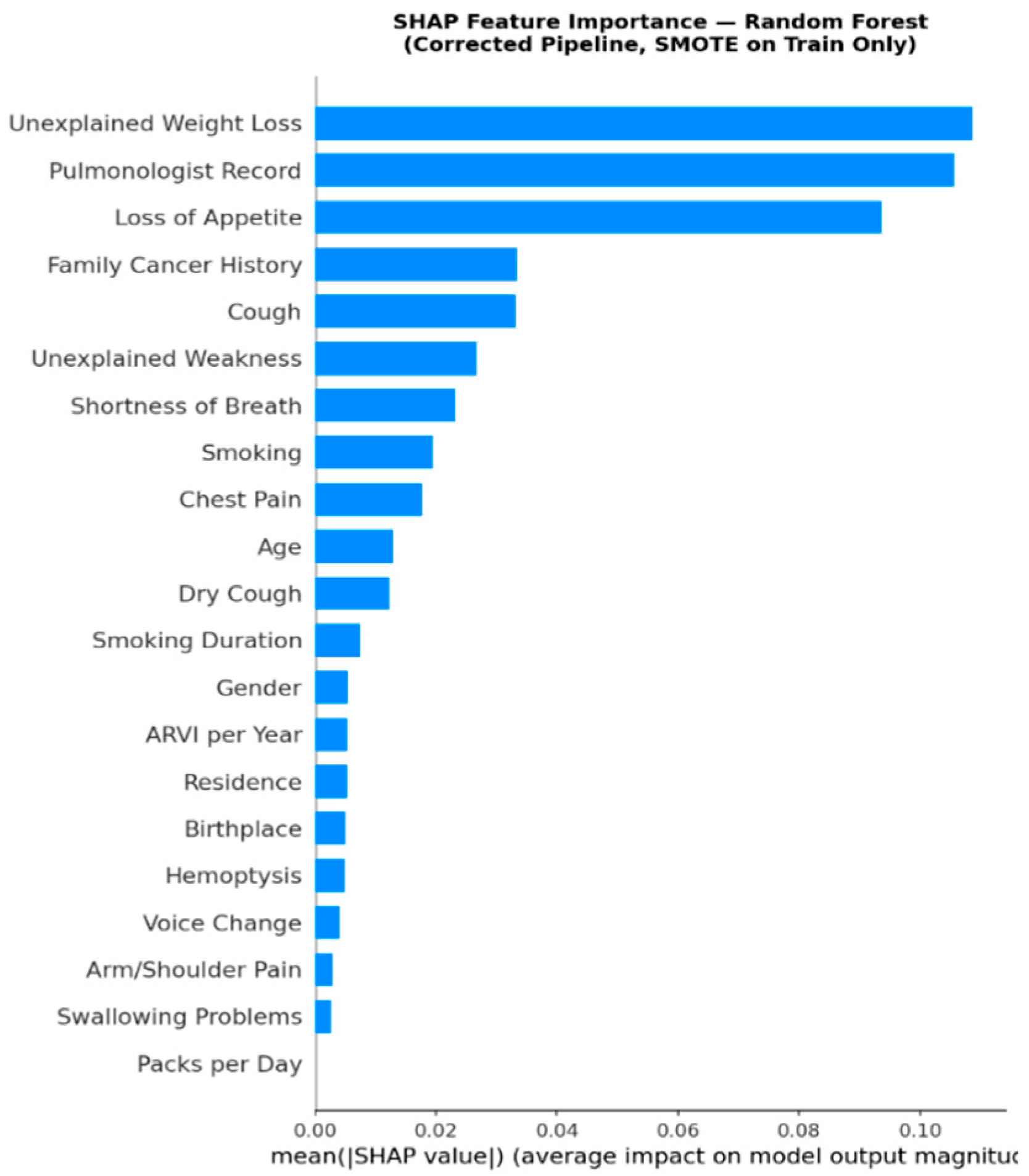
SHAP Feature Importance shows the average absolute influence of each feature on the model’s predictions. SHAP Feature Importance (Figure 7) confirms the results of the “Feature importance” section. Unexplained weight loss, Pulmonologist follow-up, and “Loss of appetite have the greatest total influence on the model’s predictions.

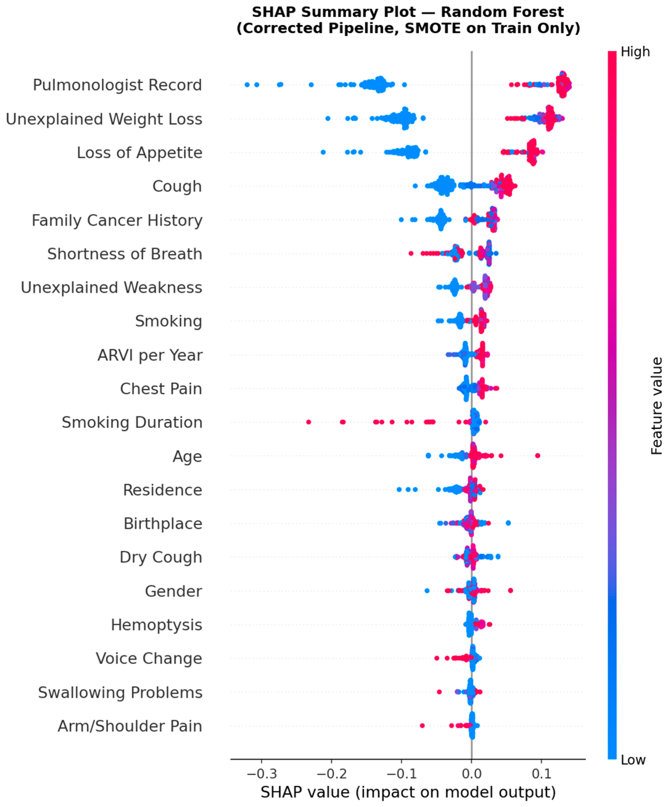
SHAP Summary Plot (Figure 8) shows the influence of each feature for each patient. The red color in the figure indicates a high feature value, while the blue indicates a low value. A position to the right of zero means an increased probability of cancer. For the feature Unexplained weight loss”, the presence of the symptom (red points, high value) increases the predicted probability of cancer (points to the right of zero), while its absence (blue points) decreases the probability (points to the left of zero). A similar pattern is observed for Pulmonologist follow-up and Loss of appetite.

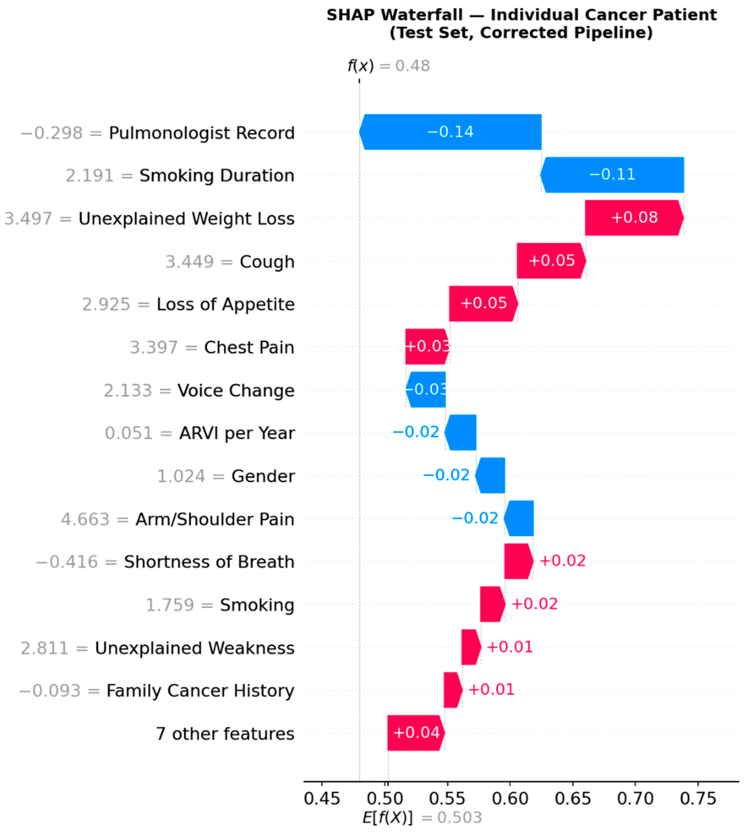
The SHAP Waterfall Plot (Figure 9) shows the explanation of the prediction for one specific lung cancer patient from the test set. The red bars shown in the figure increase the probability of cancer, while the blue bars decrease it. The model’s base prediction is 0.503. The final prediction for this patient is 0.48. Weight loss (+0.08), cough (+0.05), and loss of appetite (+0.05) increase the probability of cancer, while the absence of pulmonologist follow-up (−0.14) and a short smoking duration (−0.11) decrease it.

The obtained results indicate that the key factor determining classification quality is not the choice of algorithm, but the structure and volume of the initial data. In the studied dataset, the proportion of the positive class is less than 4% (8 out of 216 observations), which creates extremely unfavorable conditions for training machine learning models. This problem is widely described in the literature as the “accuracy paradox”: a model that predicts all observations as belonging to the majority class automatically achieves a high Accuracy value, while having no clinical value whatsoever. The cross-validation results confirm this thesis. In most splits, the models do not detect any lung cancer cases, and the average F1-Score remains low. This is explained by the fact that when splitting the training set into five parts, each training group contains only 4–5 lung cancer patients. Under such conditions, the models are unable to form the stable patterns necessary for the reliable detection of the minority class. Consequently, with an extremely small number of positive observations, even modern balancing methods cannot ensure stable classification quality. The results obtained confirm that the main limitation is not the choice of algorithm but the insufficient data volume.

On the test set, the models exhibit substantially different behavior depending on the metric used. SVM achieves the best F1-Score (0.667) and is the only model that does not produce false-positive predictions (Precision = 1.000). This means that all patients classified by the SVM model as belonging to the risk group are, in this sample, truly in the positive class. This result is consistent with the known effectiveness of SVMs on small samples, as the algorithm constructs a separating hyperplane that maximizes the margin between classes, thereby helping mitigating overfitting with a limited number of training examples.

KNN is the only model that detects both real lung cancer cases (Recall = 1.000). However, this result comes at the cost of six false-positive predictions. This indicates high sensitivity and low specificity in this model, which is typical of distance-based algorithms operating small sample sizes. In the context of medical diagnostics, the choice between SVM and KNN depends on the clinical goal: SVM is preferable for the precise selection of high-risk patients, while KNN is preferable for mass screening tasks where missing disease cases is unacceptable.

Random Forest and XGBoost do not detect any cancer cases at the standard classification threshold (F1 = 0), despite their high AUC-ROC values (0.976 and 0.893, respectively). This indicates that the standard 0.5 threshold is not optimal for these models when class imbalance is severe. Individual tuning of the classification threshold based on maximizing F1-Score or Recall would significantly improve their performance. The high ROC-AUC values with zero Recall across several models indicate a mismatch between the standard classification threshold and tasks with severe class imbalance. Consequently, the SVM model achieves the best balance between sensitivity and precision among the algorithms considered. This result suggests the potential usefulness of SVM in tasks with limited medical data.

The high ROC-AUC values for Random Forest and KNN (0.976) indicate their strong ability to rank patients by risk level across different classification thresholds. At the same time, ROC-AUC does not reflect a model’s actual ability to detect the positive class at a fixed threshold, which is especially important in the presence of severe class imbalance. In particular, Random Forest achieves an AUC-ROC of 0.976 with zero Recall, underscoring the limitations of this metric for assessing a model’s clinical effectiveness. In this regard, the Precision–Recall AUC (PR-AUC) is also analyzed, as it provides a more informative metric under class imbalance because it does not account for true-negative observations, focusing directly on the quality of rare positive class detection. Unlike ROC-AUC, PR-AUC more accurately reflects model quality in conditions of a rare positive class. KNN achieves the best PR-AUC of 0.667, followed by SVM at 0.611. Both values significantly exceed the baseline classifier’s level (0.045), indicating the models’ real predictive ability. Therefore, the combined use of AUC-ROC and PR-AUC provides a more complete and objective assessment of model quality in medical diagnostic tasks with imbalanced classes.

The application of SMOTE partially compensates for class imbalance by generating synthetic observations of the minority class via linear interpolation between existing examples. However, in this study, the effectiveness of SMOTE is limited by the extremely small number of initial positive observations, as the training set contains only 6 lung cancer patients. Under such conditions, all synthetic observations are generated from a limited number of real examples, which significantly reduces their diversity and fails to adequately reflect the disease’s clinical variability. Furthermore, the number-of-neighbors parameter must be reduced to k = 3 to ensure that the algorithm works with this data volume. These further limit the space of synthetic observations. As a result, SMOTE is a necessary but insufficient tool for extremely small minority-class samples.

The consistency of results from three independent methods—Feature Importance (Random Forest and XGBoost), SHAP analysis, and comparative patient profiling—significantly increases the reliability of conclusions regarding clinically significant predictors of lung cancer. All three methods consistently identify “Pulmonologist follow-up”, “Unexplained weight loss”, and “Loss of appetite” as leading predictors. These symptoms belong to the group of constitutional signs of oncological diseases, known as cachexia-anorexia syndrome, which is observed in 40–80% of patients with malignant neoplasms. The differences in mean values of these features between patient groups confirm their strong association with the presence of lung cancer in this sample.

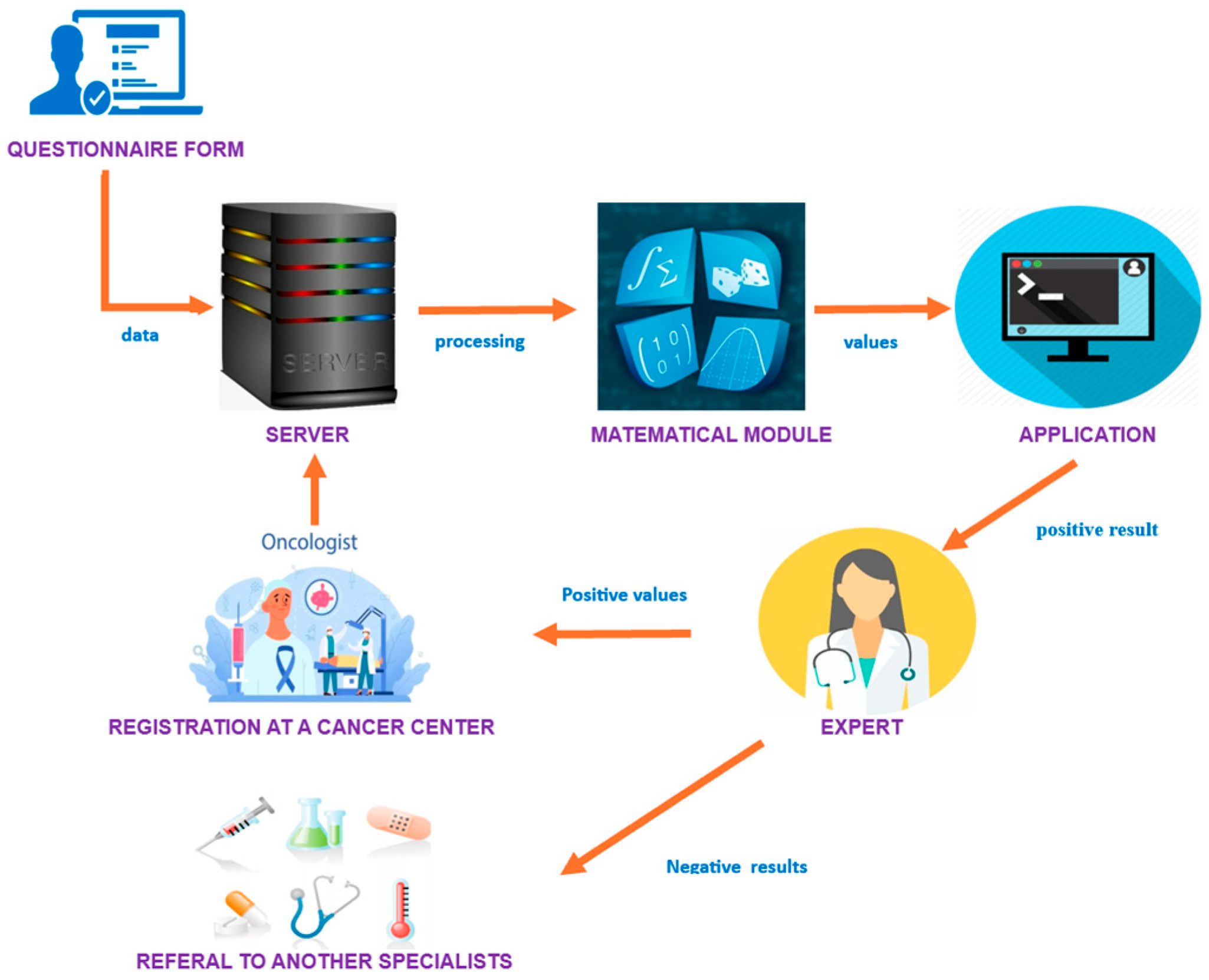
This study has several limitations that must be considered when interpreting the results. The main limitation is the extremely small number of positive cases (n = 8), which significantly reduces the statistical reliability of the metrics. The training set contained just six positive cases, raising concerns about overfitting when using SMOTE, because creating synthetic samples from only six observations might not accurately reflect the real distribution of lung cancer cases. Moreover, the independent test set included only two positive cases, which is insufficient for a statistically sound assessment of the model’s ability to generalize. As a result, all reported performance metrics, such as AUC-ROC and F1-Score, should be viewed with caution and treated as initial estimates rather than definitive indicators of the model performance. The use of questionnaire data without clinical verification may also introduce errors in the target variable. The application of SMOTE with such a small number of observations limits the quality of synthetic data. The absence of external validation prevents assessment of the model’s generalizability. Furthermore, the set of features does not include clinically significant indicators such as imaging results and laboratory data. Therefore, the results of this study should be considered preliminary and require confirmation with larger, clinically verified datasets. The main direction for further research is to increase the data volume, primarily by increasing the number of clinically verified lung cancer cases. This will improve the statistical power of the study, the stability of the models, and their generalizability. Also promising is the inclusion of instrumental diagnostics data, laboratory biomarkers, and information from medical records, which will significantly expand the information capacity of the feature space. Among methodological improvements, it is advisable to consider tuning the classification threshold based on the target metric, employing cost-sensitive learning, and calibrating probabilistic predictions. External validation on an independent clinically verified sample is a mandatory next step to confirm the applicability of the proposed approach in real clinical practice. To create an interconnected system for cancer prediction, it is necessary to build a flexible system architecture. The system architecture is shown in Figure 10 and it consists of the following modules: survey module, data storage module, data processing module, and decision-making module.

In this system, the sequence of actions is implemented as follows: for the early detection of lung cancer, patients complete a questionnaire developed by incorporating predictors that influence the risk of lung cancer development. These questionnaire results data are stored in a database, and within the mathematical module, the risk group for lung cancer susceptibility is determined using machine learning models.

Stage 4. Referral of patients at high risk of lung cancer susceptibility to a physician. Based on the modeling results, lung cancer susceptibility was determined. Patients with high lung cancer susceptibility results are given recommendations to consult a physician for further comprehensive diagnostics.

Practical implementation

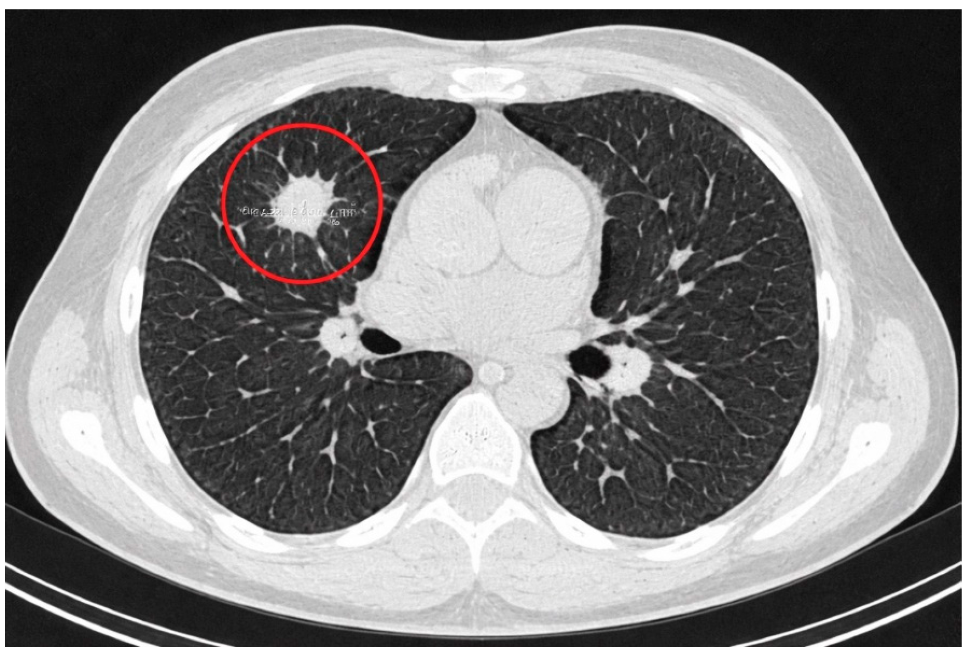
1. Patient A completed a questionnaire to determine their risk of lung cancer susceptibility. Based on the questionnaire results, a value of 0.942564 was obtained, classifying the patient into class 4—very high risk. The patient was given recommendations to consult a physician. The patient was referred to a clinic for fluorography, where a suspicious opacity was detected → referred for a CT scan. Figure 11 shows a computed tomography scan of the chest organs of patient A. As shown in this figure, there is a solitary lesion in the upper lobe of the right lung, measuring 2.2 × 1.8 cm. This lesion shows no signs of lymph node involvement.

Surgical treatment was performed: Right upper lobectomy. Postoperative period: Uncomplicated. Diagnosis: Cancer of the upper lobe of the right lung. Stage IA2 (T1bN0M0).

2. Patient B completed a questionnaire to determine their risk of lung cancer susceptibility. Based on the questionnaire results, a value of 0.912779 was obtained, classifying the patient into class 4—very high risk. The patient was given recommendations to consult a physician.

Recommended: High-resolution CT, spirometry, and a pulmonologist consultation. The series of chest CT scans showed diffuse interstitial fibrosis.

3. Patient C completed a questionnaire to determine their risk of lung cancer susceptibility. Based on the questionnaire results, a value of 0.936779 was obtained, classifying the patient into 4—very high risk. The patient was given recommendations to consult a physician. CT shows approximately: local linear fibrous strands and pleural plaques. This corresponds to residual changes after inflammation. Follow-up, physical therapy, and a repeat examination in 6–12 months were recommended.

4. Patient D completed a questionnaire to determine their risk of lung cancer susceptibility. Based on the questionnaire results, a value of 0.938719 was obtained, classifying the patient into class 4—very high risk. The patient was given recommendations to consult a physician.

CT revealed a single, rounded calcification in the lungs and lymph nodes.

It should be noted that Patients B, C, and D received high-risk classifications from the model (scores above 0.91), yet CT imaging did not confirm malignancy. This outcome is consistent with the known behavior of machine learning models trained on severely imbalanced data, as the model tends to overpredict the positive class to minimize missed cancer cases. These cases highlight the importance of combining questionnaire-based screening with clinical imaging confirmation. They should not be interpreted as model failures, but rather as an expected characteristic of a high-sensitivity screening tool designed to minimize false negatives. The presented clinical cases are illustrative examples only and do not constitute formal clinical validation.

4. Discussion

The early diagnosis of oncological diseases is one of the pressing tasks today. Mortality from lung cancer is among the highest across cancer types. In this regard, early diagnosis of lung cancer has important social significance.

This article addresses the problem of early lung cancer diagnosis using classical machine learning algorithms. Data on lung cancer diagnosis were used as predictors for the models, including family cancer history, pulmonologist follow-up, smoking duration, and frequency of acute respiratory viral infections.

In this study, a comparative analysis of six machine learning algorithms for predicting lung cancer from questionnaire data was conducted. A correct analysis scheme was applied: the data were split in an 80%/20% ratio, the SMOTE method was used only for the training data within a pipeline, and the final evaluation was performed on an independent test set. According to the ROC-AUC metric, the Random Forest model showed the best result (0.976). In terms of the F1-score and precision for the positive class, the support vector machine (SVM) demonstrated the highest performance (F1 = 0.667, Precision = 1.000). In turn, gradient boosting provided the most balanced results across key clinical metrics. A SHAP analysis initially found three factors that might be linked to lung cancer risk in this sample: pulmonologist follow-up, unexplained weight loss, and loss of appetite. These early results align with observations in clinical settings and suggest that the use of ensemble machine learning methods in medical diagnostics warrants further study. However, it is important to confirm these findings with larger datasets.

The overall results indicate that machine learning techniques could be useful for lung cancer screening using questionnaire data, especially with a larger training sample and external validation beyond clinical settings.

Further research will aim to include an image-scanning module in this system that analyzes patients’ computed tomography scans to determine tumor localization and neoplasm malignancy.

5. Conclusions

The aim of this study was to identify a predisposition to lung cancer and the factors that most significantly influence the risk of developing lung cancer. The input data for the study were taken from a preliminary questionnaire protocol for lung cancer diagnosis. A survey was conducted using this early diagnostic scheme, as a result of which input data for modeling were obtained. As a result of modeling, a result was obtained that shows the percentage of lung cancer susceptibility. This study conducted a comparative analysis of six machine learning algorithms for lung cancer prediction using questionnaire data.

According to the ROC-AUC metric, the Random Forest algorithm demonstrated the best results (0.976). In terms of the F1-score and precision for the positive class, the support vector machine (SVM) lead (F1 = 0.667, Precision = 1.000). At the same time, gradient boosting showed the most balanced quality across clinically significant indicators.

Using a SHAP analysis, three preliminary predictors potentially associated with lung cancer risk in this sample were identified: seeing a pulmonologist, unexplained weight loss, and a loss of appetite. These preliminary findings are consistent with clinical practice and suggest the potential for the interpretability of ensemble machine learning models in medical diagnostic tasks, though validation on larger, clinically verified datasets is required.

The obtained preliminary results suggest the potential of using machine learning methods for lung cancer screening based on questionnaire data, especially with an increase in the size of the training sample and external clinical validation.