XCrime-LLM: An Explainable Spatio-Temporal Crime Prediction Framework

Abstract

Crime prediction can support proactive public-safety planning, but practical deployment also requires outputs that are reliable and explainable. This study proposes XCrime-LLM for next-week crime occurrence prediction, in which engineered spatio-temporal features are serialized into a fixed prompt format and used to fine-tune GPT-4.1-mini to produce schema-guided JSON outputs from New York City Police Department (NYPD) incident records. The proposed XCrime-LLM framework is evaluated against prompting and trained baselines in New York City and further examined for cross-city transfer in Chicago. Supervised fine-tuning improved GPT-4.1-mini compared with the prompting baselines, increasing Micro-F1 from 0.7478 to 0.8095 and Macro-F1 from 0.7485 to 0.8075, while remaining competitive with the trained baselines. In the cross-city evaluation on Chicago, the fine-tuned GPT-4.1-mini outperformed the base GPT-4.1-mini without further fine-tuning or city-specific adaptation, raising Micro-F1 from 0.8277 to 0.8650 and Macro-F1 from 0.8693 to 0.9020. For explainability under black-box access, KernelSHAP identified last28_mean as the most influential feature across all crime types, while targeted ablation provided additional evidence of the model’s reliance on this feature. These findings suggest that the framework supports competitive next-week crime occurrence prediction while remaining explainable under black-box deployment constraints.

1. Introduction

Crime remains a major public-safety concern with substantial social and economic consequences for communities and public institutions [1,2,3]. A 2021 aggregate estimate placed the annual cost of crime in the United States at $4.71–$5.76 trillion, highlighting both the scale of the burden and the need for more proactive and targeted public-safety planning [4]. This has led to an increasing interest in predictive approaches that can support earlier intervention by anticipating when and where crime is likely to occur [5]. Because crime is often concentrated in particular places and changes over time, spatio-temporal crime prediction has been studied as a way to estimate near-term crime occurrence and support resource allocation [6,7,8].

Existing studies have explored crime prediction using statistical, machine learning, and deep learning approaches [7,9,10]. These methods differ in their modeling assumptions and predictive capabilities. Statistical approaches are commonly used to examine crime trends and associations, whereas machine learning and deep learning models can capture more complex spatio-temporal relationships [7,8,10,11]. However, operational decision support settings require more than predictive accuracy; model outputs should also be sufficiently reliable and explainable to support human decision-making [12,13,14]. This concern is especially important for complex models whose reasoning is not directly observable.

Explainable artificial intelligence (XAI) approaches are commonly categorized into interpretable-by-design models and post hoc explanation methods [12]. Interpretable-by-design models are structured to be relatively understandable, whereas post hoc methods are applied after model training to explain the behavior of complex or black-box models [12,15]. In black-box settings, model-agnostic post hoc methods are particularly useful because they generate explanations using only model inputs and outputs. Common examples include Local Interpretable Model-agnostic Explanations (LIMEs) and Shapley Additive Explanations (SHAP) [16,17].

Alongside developments in predictive modeling and explainability, recent work has begun to examine whether LLMs can support structured prediction tasks. In this setting, tabular or feature-based records are converted into text-based inputs, and predictions are guided through prompting or fine-tuning [18,19]. Recent studies on LLMs for tabular data have reported promising performance on structured prediction benchmarks [20,21,22]. Early studies have also explored LLMs in spatio-temporal urban prediction and smart policing contexts [23,24]. However, the use of LLMs for spatio-temporal crime occurrence prediction remains underexplored, particularly in structured multi-label settings that require machine-readable outputs and post hoc explanations suitable for black-box settings. This study proposes XCrime-LLM, a structured LLM-based framework for next-week crime occurrence prediction using engineered spatio-temporal features. The framework uses schema-guided prompting to produce structured JSON outputs for multi-label prediction and supports post hoc explainability under API-only black-box access.

The main contributions of this study are summarized as follows:

• Propose XCrime-LLM, a structured LLM-based framework for next-week crime occurrence prediction that combines engineered spatio-temporal features, schema-guided prompting, and structured JSON outputs under API-only black-box access.
• Evaluate XCrime-LLM against prompting and trained baselines, including zero-shot and few-shot GPT-4.1-mini, XGBoost, and multilayer perceptron (MLP), using New York City crime data, and examine cross-city transfer in a Chicago evaluation setting.
• Introduce a black-box-compatible explainability procedure for XCrime-LLM that extracts label-wise decision scores from decision-token log-probabilities under API-only black-box access and enables KernelSHAP-based feature attribution for multi-label predictions.
• Assess explanation faithfulness through targeted test-time ablation by examining whether highly ranked KernelSHAP features correspond to measurable changes in prediction behavior and overall performance.

The remainder of this paper is organized as follows. Section 2 reviews the related work. Section 3 presents the proposed methodology, and Section 4 describes the experimental setup. Section 5 reports the predictive and explainability results. Finally, Section 6 concludes the paper and outlines directions for future work.

2. Related Work

This section reviews related work in four research areas. It begins with spatio-temporal crime prediction for public-safety planning, including statistical baselines, machine learning approaches, and deep spatio-temporal models. It then reviews explainable AI (XAI) methods for spatio-temporal prediction. Finally, recent LLM-enabled urban prediction and crime decision support frameworks are reviewed, highlighting the need for explainable LLM-based prediction under API-only access.

2.1. Spatio-Temporal Crime Prediction for Decision Support

Spatio-temporal crime prediction estimates when and where incidents are likely to occur to support public-safety planning, such as patrol deployment and resource allocation [7,9]. Because crime exhibits spatial clustering and temporal regularities [7,25], many methods formulate prediction at the region and time-window level [7]. Prior work addresses this objective through hotspot prediction, crime-count prediction, and crime occurrence prediction [7,14]. Among these tasks, crime occurrence prediction is closely aligned with operational decision support because it estimates whether an incident is expected to occur within a defined future window.

2.1.1. Statistical and Density-Based Approaches

Common statistical baselines transform historical incidents into risk estimates through transparent constructions that support operational interpretability [7]. Kernel Density Estimation (KDE) and its spatio-temporal extension smooth past events over space and time to produce hotspot risk surfaces [7]. Han et al. [11] extend this idea with a cyclically adjusted spatio-temporal KDE that accounts for periodic temporal patterns. These methods are relatively interpretable because predicted risk can be traced directly to the spatial and temporal distribution of prior incidents. Complementing density-based approaches, near-repeat frameworks capture temporary risk elevation near recent incidents, reflecting event dependence relevant to occurrence forecasting [25]. He et al. [25] operationalize this structure by modeling incident pairs as a transmission network and mining dominant spatial transmission routes between grid regions. While transparent and operationally useful, these baselines have limited capacity to incorporate diverse feature sets, motivating the use of supervised machine learning [7,9].

2.1.2. Classical Machine Learning Approaches

With the availability of richer crime records, subsequent work has leveraged engineered spatio-temporal and incident-level features to predict target outcomes [7,9]. Within this tabular paradigm, Almuhanna et al. [8] study neighborhood-level crime prediction in New York City using spatial data analysis and evaluate multiple classical classifiers, such as support vector machines (SVMs), random forests, and XGBoost. Mytheli et al. [26] compare logistic regression with boosting-based models and report Light Gradient Boosting Machine (LightGBM) as the strongest performer. Moving beyond individual learners, Kshatri et al. [27] explore stacking, where a meta-learner integrates the outputs of multiple base models to improve performance over single classifiers. While these models can improve predictive accuracy, their decision logic is typically less transparent than that of statistical baselines, which motivates the use of post hoc explanations [12,16,17]. In addition, classical ML approaches often rely on manual feature design and may miss multi-scale spatio-temporal structure, motivating deep spatio-temporal models that learn richer representations directly from data [7,10,28].

2.1.3. Deep Spatio-Temporal Learning Approaches

Deep learning methods model crime patterns through representations learned directly from data, enabling the capture of nonlinear dynamics and multi-scale dependencies [7,9]. Early work emphasized temporal sequence modeling with attention mechanisms. Huang et al. [10] propose DeepCrime, which jointly embeds spatial, temporal, and categorical signals and models crime dynamics using an attentive hierarchical recurrent network that weights different historical periods by their relevance.

Subsequent work adopted transformer-style self-attention to capture long-range dependencies across space and time [29]. Wu et al. [28] introduce STtrans, a hierarchically structured spatial–temporal transformer that models inter-region and temporal dependencies jointly, and incorporates a cross-category fusion module to capture relationships among crime types.

Because crime risk is shaped by spatial interactions among neighboring regions, graph-based models represent regions as nodes and encode these interactions as edges [30,31]. Rayhan et al. [31] propose AIST, which uses hierarchical graph attention for region representations and feature graph attention for external signals. Sun et al. [32] propose AGL-STAN, which learns inter-community crime dependencies through adaptive graph learning and uses time-aware multi-head self-attention to model temporal influences across historical crime incidents. Although such attention-based mechanisms can improve representation learning, attention weights are not generally regarded as faithful explanations of model decisions [33,34], which limits their utility for behavioral accountability.

To model higher-order interactions, Xia et al. [35] propose ST-SHN, integrating hypergraph learning with graph-structured message passing to encode crime-type relationships. Li et al. [36] propose ST-HSL, which combines multi-view spatio-temporal encoding, hypergraph-based global dependency modeling, and dual-stage self-supervised learning to address sparse and skewed crime data. Liang et al. [37] propose HCL, which uses contrastive learning and Hawkes-enhanced temporal modeling to capture crime-type co-occurrence, neighborhood influence, and time-decaying crime dependencies. Tang et al. [38] propose STExplainer, which enhances spatio-temporal graph neural networks with explainability by identifying influential spatial and temporal substructures. As these models grow in complexity, generating faithful forecast-level explanations becomes increasingly difficult, reinforcing the need for post hoc explanation methods accompanied by explicit faithfulness validation [12,39,40]. This challenge becomes more pronounced when model behavior must be explained without direct access to internal model components.

2.2. Explainable AI for Spatio-Temporal Prediction

As spatio-temporal crime predictors grow more complex, explainability becomes increasingly important in decision support contexts [12,13,14]. A common strategy is post hoc explanation, in which the trained predictor is kept fixed and a separate method is applied to explain individual forecasts and global feature effects [12,14]. Methods such as LIME [16] and SHAP [17] are widely used for this purpose because they provide instance-level feature attributions and can also support broader summaries of feature influence.

Despite their widespread use, post hoc attributions are not guaranteed to faithfully reflect a model’s decision logic and can be unreliable without explicit validation, particularly when inputs are correlated, as is common in spatio-temporal settings [39,40,41]. Attribution methods can be complemented with behavioral tests, such as targeted perturbations or feature interventions, to assess whether highlighted features are associated with consistent and meaningful changes in predicted outputs. These considerations are especially important when models are not accessible for internal inspection [42], making behavioral validation particularly relevant for black-box prediction settings.

In crime prediction, post hoc attribution methods have been applied in several recent studies. Acampora and Vitiello [43] use LIME for instance-level explanations of crime-rate predictions and highlight the need to extend explainability to spatial tasks. Kim et al. [44] combine XGBoost with SHAP to produce place-based crime risk maps and assess CCTV installation adequacy. Chen et al. [45] apply SHAP to explain mobility-driven variation in neighborhood-level theft risk, showing that feature importance patterns can shift across spatial and temporal contexts. Khalfa et al. [46] compare multiple post hoc explanation methods for weekly micro-place burglary hotspot prediction, providing guidance on method selection for different decision objectives.

Across these studies, post hoc attribution is applied to structured feature predictors for which usable model outputs or scores are available. However, when predictions are generated by an LLM accessed through a hosted API, neither internal parameters nor continuous output scores are directly available, making standard SHAP-style attribution less straightforward.

2.3. LLM-Enabled Crime Prediction and Decision Support

Recent work beyond the crime domain has shown that LLMs can be applied to structured and tabular prediction by serializing feature–value pairs into text prompts and generating task-specific structured outputs [20,21,22]. Although these studies are not crime-specific, they motivate the use of LLMs as predictors for engineered features when the task and output format are well specified. In urban and spatio-temporal applications, LLMs have also been incorporated into prediction and decision support pipelines, including systems that produce machine-readable outputs for downstream integration [47].

Li et al. [23] propose UrbanGPT, which adapts an instruction-tuned LLM to spatio-temporal urban forecasting under limited labeled data. The model integrates a spatio-temporal dependency encoder and aligns its representations with the LLM through special spatio-temporal tokens, enabling structured spatio-temporal signals to be consumed within the language-model interface. Across cross-region (unseen-region) and cross-city evaluations, UrbanGPT reports strong zero-shot generalization and improved performance over baseline methods, suggesting that LLM-based predictors can transfer some spatio-temporal patterns beyond the training data.

Beyond LLMs as predictors, Heredia et al. [48] integrate an LLM into an interactive visual analytics system to assist analysts in interpreting spatio-temporal crime anomalies on graph-structured urban data. Anomalies are detected using an interpretable Space-Time Autoregressive Moving Average (STARMA) forecasting model, where residual deviations from one-step-ahead predictions are flagged as anomalous. The LLM then produces context-aware explanations grounded in localized spatio-temporal information provided by the interface. Case studies illustrate how the system can surface plausible links between anomalies and localized contextual factors.

Focusing on operational decision support workflows, Sarzaeim et al. [24] propose an LLM-assisted smart policing framework that converts structured incident records into natural-language descriptions through prompt engineering and constructs an instruction dataset for fine-tuning. They evaluate zero-shot and few-shot prompting, as well as instruction fine-tuning, for crime-type classification using API-based LLM interactions. Their experiments suggest that fine-tuning can improve performance in some settings, although results are dataset-dependent, and they note that clearly specifying the task and desired output format can improve prompting performance.

Despite this progress, feature-level explainability for fine-tuned LLM predictors under API-only access remains underexplored in crime and related public-safety contexts. In particular, obtaining stable label-wise decision scores for SHAP-style attribution and validating explanations against observable model behavior remain open challenges. Existing LLM-based prediction and decision support frameworks therefore provide limited support for explainable, behaviorally validated prediction in operational settings.

Table 1. Comparison of representative studies with XCrime-LLM.

Study	Task/Method Focus	LLM Pred.	Model Expl.	Faith.
Han et al. [11]	Hotspot forecasting/statistical KDE	×	×	×
Almuhanna et al. [8]	Neighborhood crime prediction/classical ML	×	×	×
Tang et al. [38]	Spatio-temporal GNN/subgraph explanation	×	✓	×
Rayhan et al. [31]	Crime prediction/attention-based deep model	×	✓	×
Kim et al. [44]	Crime risk mapping/XGBoost-SHAP	×	✓	×
Khalfa et al. [46]	Burglary hotspot prediction/XAI comparison	×	✓	×
Li et al. [23]	Urban forecasting/fine-tuned LLM	✓	×	×
Heredia et al. [48]	Crime anomaly analysis/LLM-generated contextual explanation	×	×	×
Sarzaeim et al. [24]	Smart policing/LLM-based crime classification	✓	×	×
XCrime-LLM	Schema-guided next-week type-specific crime occurrence prediction	✓	✓	✓

Note: LLM Pred. = LLM used for prediction or classification; Model Expl. = explicit explanation or interpretation of predictive model behavior; Faith. = explicit faithfulness or behavioral validation; ✓ = included; × = not included.

summarizes representative studies across the reviewed topics and compares them along the dimensions most directly related to this study. The table positions XCrime-LLM relative to prior work by indicating whether each study includes LLM-based prediction, model explanation, and faithfulness assessment. While the selected studies address crime prediction, model explanation, or LLM-enabled analysis, XCrime-LLM integrates LLM-based prediction, feature-level explanation, and faithfulness assessment within a unified framework under API-only black-box access.

3. Methodology

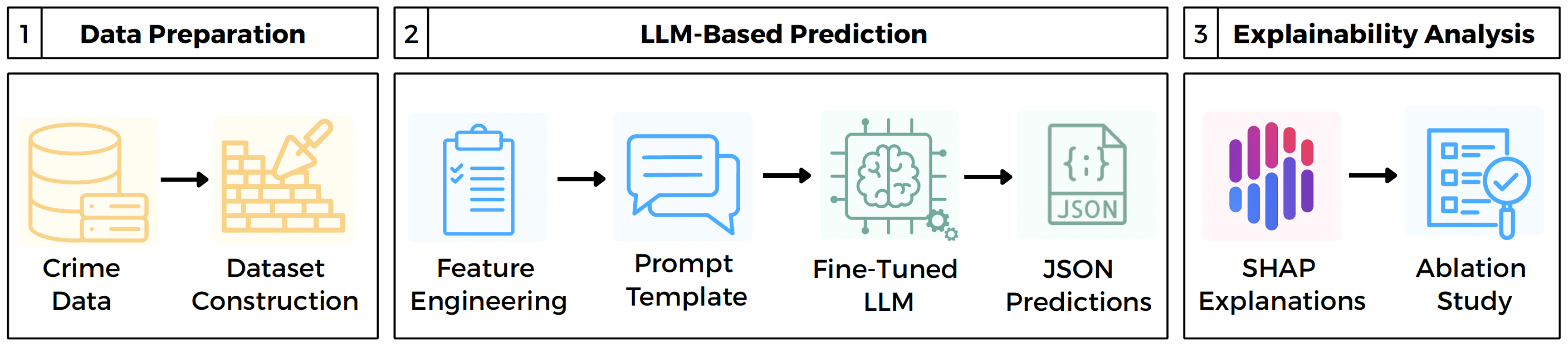
This section presents XCrime-LLM, the proposed framework for explainable spatio-temporal crime prediction. As illustrated in Figure 1, the framework comprises three main components: data preparation, LLM-based prediction, and explainability analysis. The data preparation component converts raw crime records into a structured prediction dataset. The LLM-based prediction component then converts engineered spatio-temporal features into schema-guided prompts and passes them to the fine-tuned GPT-4.1-mini predictor. The predictor returns next-week crime occurrence predictions as a JSON output. Finally, the explainability analysis component uses SHAP explanations and targeted ablation to examine the feature-level evidence and behavioral relevance of the generated predictions.

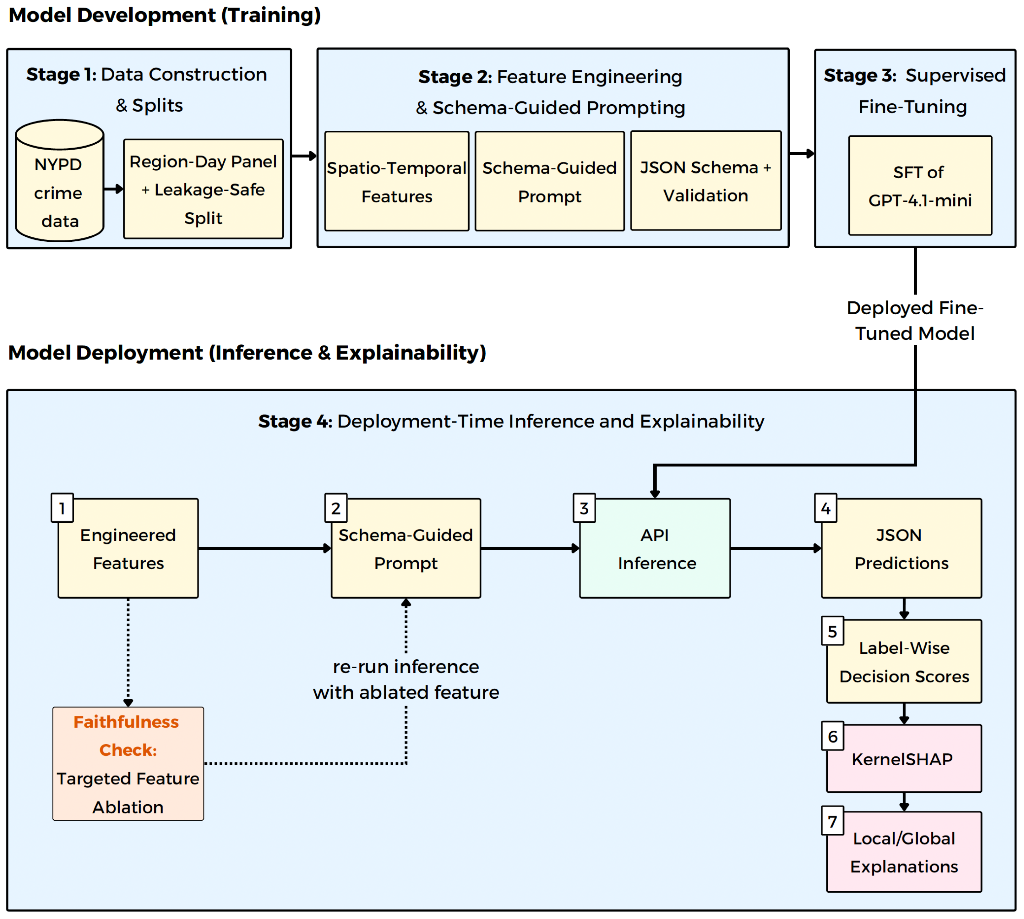
The operational implementation of XCrime-LLM is organized into four stages, as presented in Figure 2, starting from raw incident-level NYPD complaint records [49].

Stage 1 constructs a region–day panel from these records, formulates the task as supervised multi-label prediction, and partitions the timeline into chronological training, validation, and test splits to prevent data leakage.

Stage 2 computes spatial and temporal features for each (region_id, t) anchor using only information available up to day t − 1 and then serializes them through a fixed schema-guided prompting template that constrains the model to return structured JSON outputs.

Stage 3 applies supervised fine-tuning (SFT) to train GPT-4.1-mini to map the engineered inputs to schema-guided JSON outputs for next-week crime occurrence prediction. This stage uses the same schema-guided input–output interface defined in Stage 2, so fine-tuning changes the learned prediction behavior while preserving the structured prompt and JSON response format used during deployment.

Stage 4 provides the explainability component of XCrime-LLM under black-box API access. In this workflow, engineered features are first serialized according to the same schema-guided prompting template as in training and then provided to the fine-tuned GPT-4.1-mini predictor through API inference. The predictor returns next-week crime occurrence predictions as a schema-guided JSON output. Label-wise decision scores are first derived from decision-token log-probabilities [50,51] and used with KernelSHAP [17,52] to estimate feature attributions for each crime type. Model reliance on the top-ranked feature for each crime type is then assessed through targeted test-time ablation [40,41]. In this step, inference is repeated after replacing the selected feature to examine whether features that KernelSHAP identifies as important are associated with changes in the model’s predictive behavior.

3.1. Stage 1: Data Construction and Leakage-Safe Splits

This stage constructs the region–day representation, defines the next-week crime occurrence prediction task, and applies leakage-safe chronological splitting. Because the original NYPD complaint data are incident-level records rather than directly usable prediction samples, they are transformed into fixed prediction anchors, in which each anchor represents a specific region on a specific day.

3.1.1. Spatial Grid Construction and Region–Day Panel

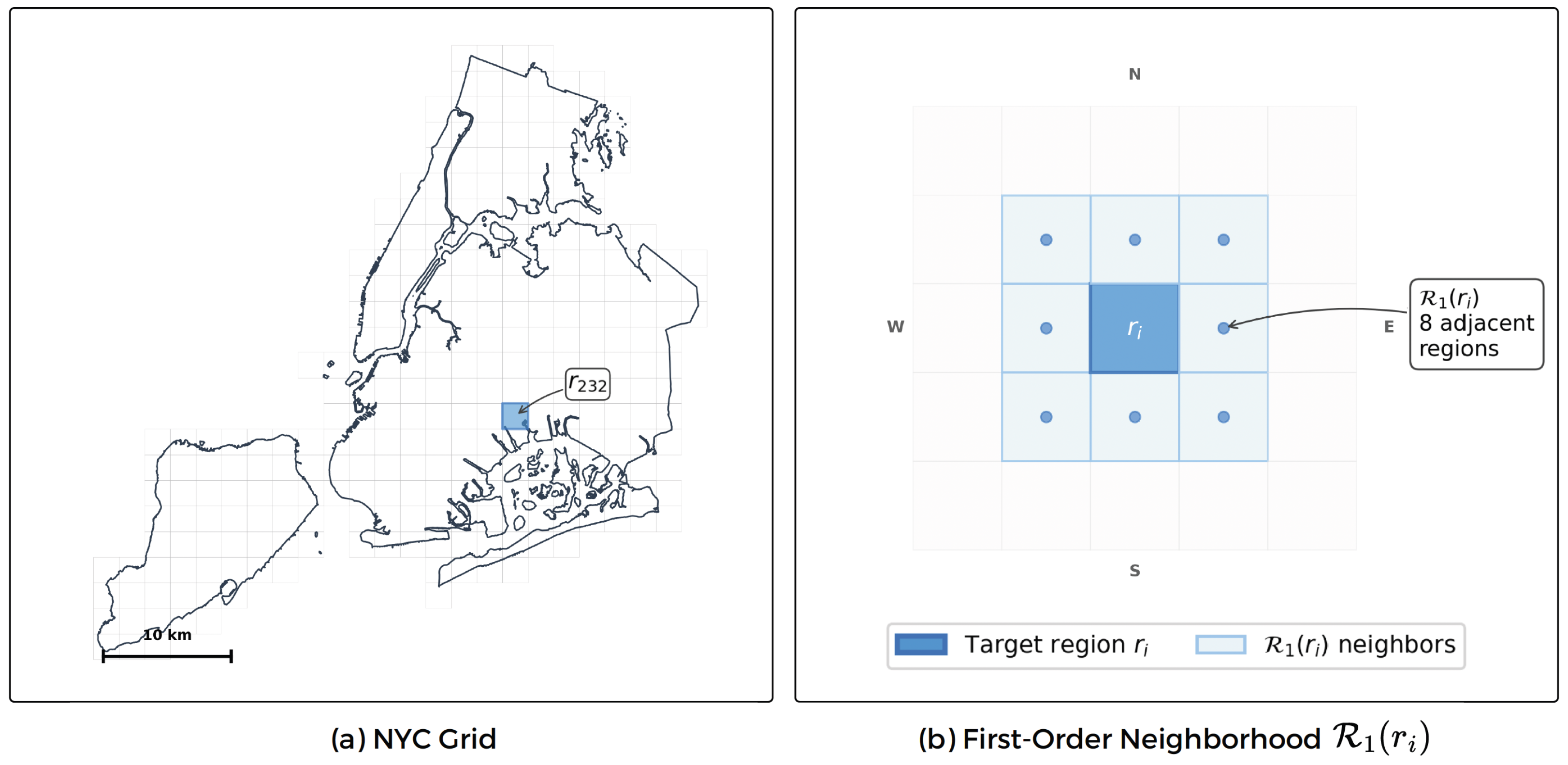
To ensure consistent physical distances across spatial units, incident coordinates are projected to a meter-based local coordinate reference system (CRS; NAD83/New York Long Island). New York City is then discretized into a regular 2 km × 2 km grid, balancing spatial granularity against sparsity in daily counts while retaining neighborhood-level variation, as illustrated in Figure 3. This grid representation also defines the first-order neighborhood $R_1\left(r_i\right)$ for each target region $r_i$: the eight surrounding cells shown in Figure 3b are used later to construct spatial neighborhood features.

The grid is fixed to the NYC bounding box, with each cell assigned a deterministic region_id. Only land cells within the NYC polygon are retained, including cells with zero incidents, while water-only cells are discarded. Each incident is mapped to its corresponding cell and aggregated into daily counts by region, date, and crime type. Timestamps are resolved to daily resolution, and missing region–day entries are filled with zeros to produce a complete region–day panel.

3.1.2. Prediction Anchors and Next-Week Labels

An anchor is defined as the pair (region_id, t), where t denotes the anchor day. A next-week horizon is used to align the task with short-term operational planning, where weekly forecasts can support near-term patrol allocation while remaining close enough to recent crime dynamics to preserve predictive relevance. Let $H=7$ denote the next-week horizon, and let $c_k$ denote a crime type, where k indexes the crime type. A binary target label_7d^(k)(t) = 1 is assigned if at least one incident of type $c_k$ occurs in the future window $[t+1,t+H]$, and label_7d^(k)(t) = 0 otherwise. This definition excludes same-day information and requires all H future days to be observable. Anchors whose full future window is unavailable, such as those near the dataset end, are discarded.

3.1.3. Leakage-Safe Chronological Splitting

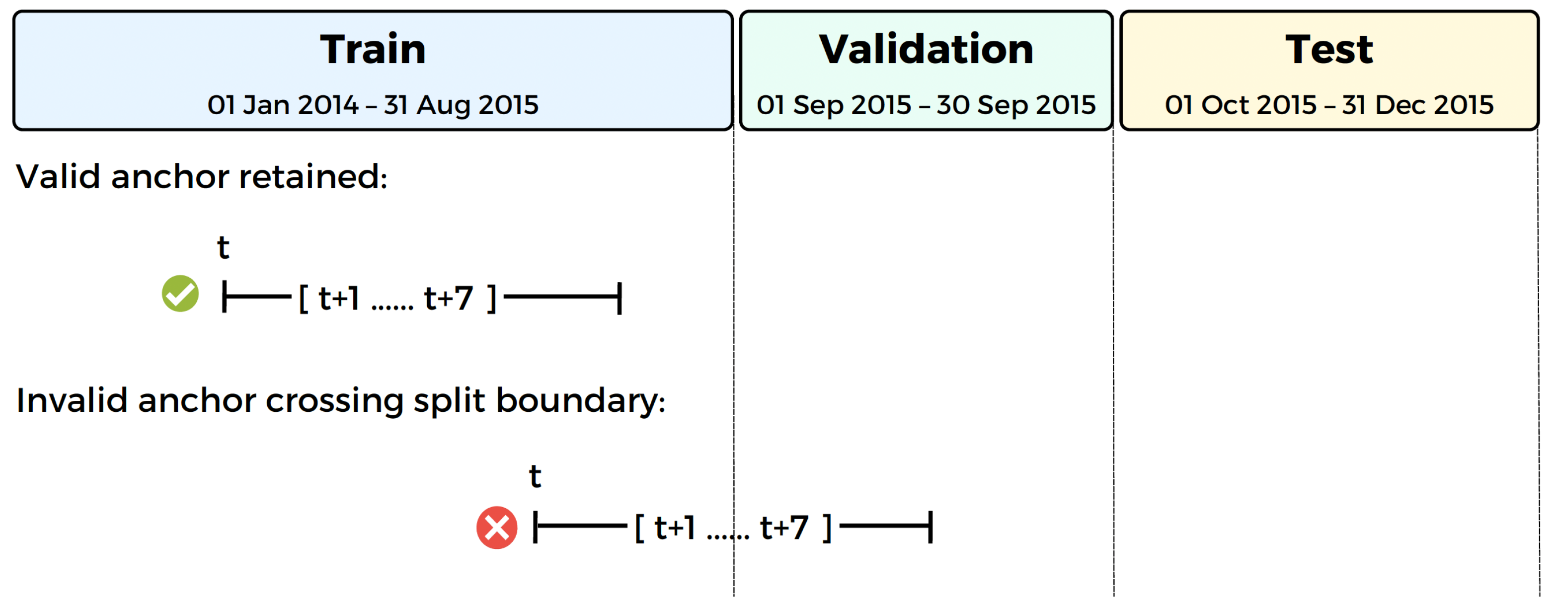
The timeline is split chronologically into disjoint training, validation, and test segments before model training and evaluation. In this study, the training segment covers 1 January 2014 to 31 August 2015, the validation segment covers 1 September 2015 to 30 September 2015, and the test segment covers 1 October 2015 to 31 December 2015. These non-overlapping segments support evaluation on later, unseen dates.

Because the prediction target uses a future seven-day window, anchors near split boundaries require special handling. For a segment ending at date T, only anchors with $t\le T-H$ are retained, where $H=7$. This ensures that the full future label window $[t+1,t+H]$ remains entirely within the same segment. After applying this rule, the retained anchor-date ranges are 1 January 2014 to 24 August 2015 for training, 1 September 2015 to 23 September 2015 for validation, and 1 October 2015 to 24 December 2015 for testing. Anchors whose future label window crosses from training into validation, or from validation into test, are discarded. Figure 4 illustrates the leakage-safe splitting rule by comparing a valid anchor, whose full seven-day label window remains within the same chronological segment, with an invalid anchor whose future label window crosses a split boundary. This prevents label leakage across chronological segments.

After the leakage-safe split is applied, anchors are additionally retained only when all four crime-type rows are available for the same (region_id, t), preserving the fixed multi-label structure used by the schema-guided prompt and JSON output.

3.2. Stage 2: Feature Engineering and Schema-Guided Prompting

This stage operates on the leakage-safe anchors produced in Stage 1 and transforms them into structured model inputs. Spatio-temporal features are computed to summarize recent intensity, medium-term history, seasonality, and neighborhood context, then serialized through schema-guided prompting for supervised fine-tuning and inference.

3.2.1. Feature Engineering

Building on the region–day panel constructed in Stage 1, each region–day anchor is transformed into a feature representation for model input. For each anchor (region_id, t) and crime type $c_k$, we compute interpretable features capturing recent incident intensity, medium-term trends, inactivity, seasonality, and local spatial context. A compact feature set is used to keep the inputs readable and to support feature attribution analysis under black-box deployment.

All history-dependent features are computed from data available up to day t − 1. In implementation, windowed statistics are computed on one-day-shifted time series to prevent the anchor day from entering its own features. Accordingly, the engineered feature vector for each (region_id, t) anchor–crime-type pair combines three feature groups: seasonality, temporal patterns, and spatial context. The resulting features are summarized in

Table 2. Engineered spatio-temporal features used in XCrime-LLM.

Group	Feature	Description
Seasonality	dow	Day-of-week indicator capturing weekly variation in crime occurrence.
Seasonality	month	Month indicator capturing broader seasonal variation.
Temporal patterns	last7_total	Total number of incidents of the same crime type in the same region during the previous seven days.
Temporal patterns	last28_mean	Mean daily number of incidents of the same crime type in the same region during the previous 28 days.
Temporal patterns	recency	Number of days since the most recent prior incident of the same crime type in the same region.
Temporal patterns	base_rate	Bounded prior rate computed from recent seven-day history.
Spatial context	R1_influence	Mean past-week crime intensity in the adjacent 1-hop neighborhood around the target grid cell.

. These engineered features serve as the structured inputs for the schema-guided prompt and as the feature set examined in the attribution analysis.

• Intensity, trend, and inactivity. Let $r_i$ denote the ith region, $c_k$ the kth crime type, and $X_{r_i,c_k,t}$ the number of incidents observed in region $r_i$ for crime type $c_k$ on day t. Short-term intensity is represented by the past-week total last7_total, denoted $S_7(r_i,c_k,t)$:

  $$S_7(r_i,c_k,t)={\displaystyle \sum _{\tau =t-7}^{t-1}}{X}_{r_i,c_k,\tau }.$$

  (1)

Medium-term trend is represented by last28_mean, defined as the mean daily count over the previous 28 days. To quantify inactivity, recency is defined as the number of days since the most recent incident of type $c_k$ in region $r_i$ before day t. Finite values are capped at 365 days to limit the influence of extreme delays and keep the feature within a bounded numeric range, while anchors with no prior observed incident are assigned the special value 9999 to denote the distinct case of no observed prior history.

A bounded prior feature, base_rate, denoted $B(r_i,c_k,t)$, is also defined by mapping $S_7(r_i,c_k,t)$ to the probability of observing at least one incident in the next-week window under a Poisson-inspired assumption. This provides a bounded prior risk score that increases with recent incident intensity, so that larger past-week counts correspond to higher estimated occurrence risk.

$$B(r_i,c_k,t)=1-exp\left(-S_7(r_i,c_k,t)\right).$$

(2)

• Neighborhood context. To incorporate local spatial dependence, the 1-hop neighborhood ${\mathcal{R}}_1\left(r_i\right)$ is defined as the set of up to eight adjacent grid cells around region $r_i$. A 1-hop neighborhood is used to capture immediate local context while limiting the influence of more distant regions. Let $r_n$ denote a neighboring region in ${\mathcal{R}}_1\left(r_i\right)$. R1_influence, denoted $I_1(r_i,c_k,t)$, is computed as the mean neighbor past-week intensity:

  $$I_1(r_i,c_k,t)={\displaystyle \frac{1}{\left|{\mathcal{R}}_1\left(r_i\right)\right|}}\sum _{r_n\in {\mathcal{R}}_1\left(r_i\right)}{S}_7(r_n,c_k,t).$$

  (3)

3.2.2. Schema-Guided Prompting and Output Schema

To support consistent prediction from engineered features under black-box API access, a fixed schema-guided prompting template is defined together with a strict schema-guided JSON output format. Because the model is used through a fixed input–output interface, consistency is enforced through the prompt structure and output schema.

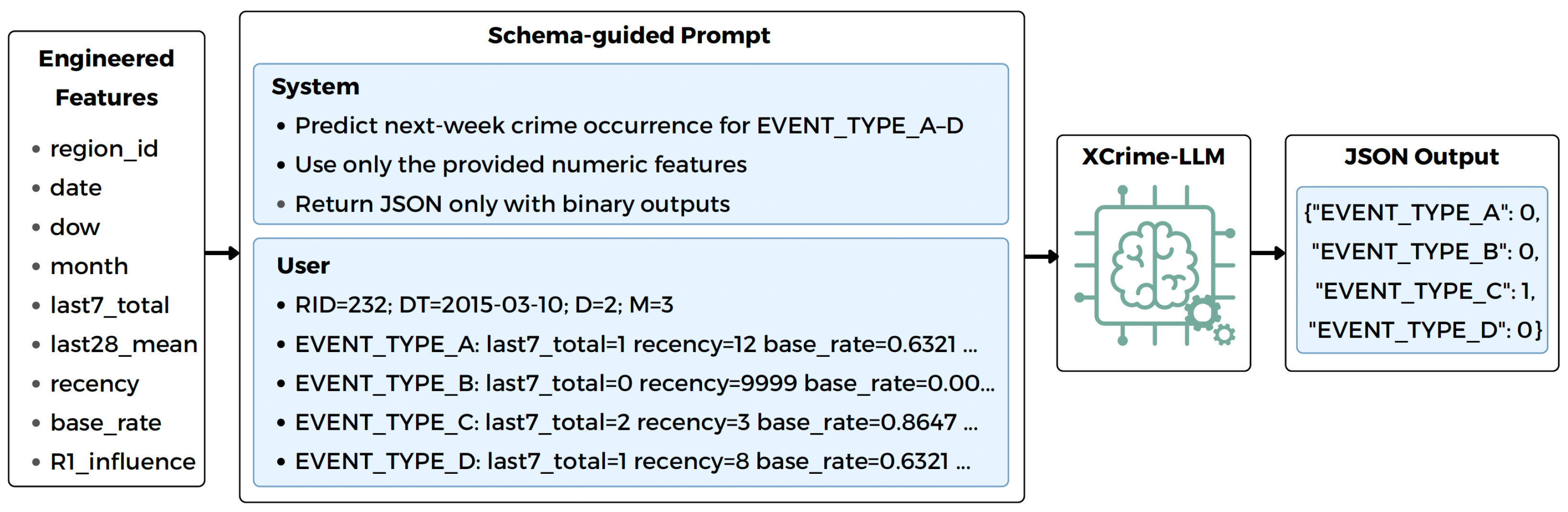
Each region–day anchor is serialized into a fixed prompt structure consisting of shared temporal indicators and four fixed-order crime-type lines corresponding to EVENT_TYPE_A–EVENT_TYPE_D. These abstract event-type identifiers are used instead of dataset-specific crime names to preserve a stable schema-guided interface and fixed label ordering across datasets, while allowing the label mapping to be defined separately for each experimental setting. The strict JSON output schema requires the same four keys with binary values for every prediction, supporting machine-readable outputs and reliable parsing during supervised fine-tuning and inference.

As illustrated in Figure 5, the engineered features are inserted into the user message, while the system message defines the prediction task, input-use constraints, and JSON-only response requirement. The fine-tuned GPT-4.1-mini predictor then uses this interface to return schema-guided JSON output containing one hard 0/1 output for each event type. This design keeps the schema-guided input and output structure consistent across supervised fine-tuning, deployment-time inference, and reliable response parsing.

• System message. The system message specifies the prediction task and output constraints: decisions are made independently for each crime-type label, only the provided numeric features may be used, and the response must consist of JSON only with exactly the required keys and binary values. Brief feature semantics are also provided where needed to reduce ambiguity during inference.
• User message. The user message begins with a compact anchor header (region_id, date, dow, month), followed by four fixed-order crime-type lines (A–D). Each line uses a fixed key–value format: EVENT_TYPE_k: last7_total=… recency=… base_rate=… R1_influence=… last28_mean=…. Numeric values are formatted deterministically, with integers for count-based fields and fixed decimal precision for continuous fields.
• Output schema and validation. The model outputs a single JSON object with four binary keys (EVENT_TYPE_A–EVENT_TYPE_D), indicating whether at least one incident of each crime type occurs in the prediction window. Responses are validated against the required keys and binary (0/1) values to support reliable downstream parsing.

The final schema-guided prompting template is established through iterative development before supervised fine-tuning, with refinements to the task instructions, feature serialization, and prompt compactness.

3.3. Stage 3: Supervised Fine-Tuning (SFT)

This stage selects the base model for XCrime-LLM and applies supervised fine-tuning to align it with the prompting template and JSON output schema defined in Stage 2. The selected model gpt-4.1-mini-2025-04-14 is trained using OpenAI’s supervised fine-tuning API so that engineered feature prompts are mapped consistently to bundled multi-label outputs.

3.3.1. LLM Selection and Fine-Tuning Rationale

Model selection focused on publicly accessible GPT-based models that support supervised fine-tuning and API deployment. The use of a GPT-based model that supports both supervised fine-tuning and API deployment is consistent with the design of XCrime-LLM. In the proposed framework, engineered spatio-temporal features are provided to the model through a fixed schema-guided prompt, and predictions are returned as a structured JSON output. Supervised fine-tuning therefore supports adapting the selected model to this fixed input–output format [53]. After fine-tuning, the model remains accessible through the provider API, preserving the black-box setting used throughout XCrime-LLM because prediction and explainability analysis are performed without access to model weights, gradients, or hidden states.

Candidate models are compared in terms of capability, cost, and inference speed. Capability is assessed through instruction-following and reasoning performance using IFBench [54], GPQA [55], and MMLU-Pro [56] as the main reference benchmarks, with AIME-2025 included as a supplementary indicator of multi-step reasoning. Cost is assessed using the API input and output pricing listed on the provider’s pricing page (accessed 24 September 2025), while speed is assessed using output tokens per second. Publicly reported benchmark scores and speed values are collected from Artificial Analysis, while pricing information is obtained from the official OpenAI model pages [57,58,59,60,61,62,63].

Table 3. Comparison of candidate GPT models considered for final model selection.

Model	IFBench	GPQA	MMLU-Pro	Price (USD, In/Out)	Speed (Output Tokens/s)	Assessment
GPT-4o-mini	31.0	42.6	64.8	$0.15/$0.60	NR	Lowest cost, but weaker capability
GPT-4o	NR	52.1	NR	$2.50/$10.00	74	Higher cost with limited comparative coverage
GPT-4.1-mini	38.3	66.4	78.1	$0.40/$1.60	101.2	Best overall balance; selected
GPT-4.1	43.0	66.6	80.6	$2.00/$8.00	109.0	Slightly stronger, but substantially costlier

Notes: NR = not reported in the consulted source or not available in a directly comparable form.

summarizes the comparison and shows how the candidate models differ in benchmark performance, API cost, inference speed, and suitability under the API-only setting of XCrime-LLM.

As shown in Table 3, GPT-4.1-mini is selected because it offers the best balance of capability, cost, and inference speed for the operational requirements of XCrime-LLM. Although GPT-4.1 achieves slightly higher benchmark scores, its substantially higher API cost makes GPT-4.1-mini more suitable for repeated inference and explainability experiments that require many API calls, while also supporting the supervised fine-tuning required by XCrime-LLM. Supervised fine-tuning is then applied to adapt the selected model to the fixed schema-guided prompting template and required JSON output format, reduce avoidable output variation, and improve schema adherence at inference time.

3.3.2. Fine-Tuning Subset Construction

To keep supervised fine-tuning manageable in terms of time and cost, the SFT training file was generated from a 30% stratified subsample of the training anchors rather than from the full training segment. Stratification was performed by month and label density, where label density denotes the number of positive labels across the four crime types at a given anchor. This reduced the number of submitted training examples by approximately 70% and limited the submitted fine-tuning run to 16,831,084 trained tokens, with an observed training cost of $84.16 on the OpenAI platform. The complete fine-tuning job lifecycle took approximately 1 h and 14 min, including file validation, fine-tuning, model creation, and post-training usage-policy evaluation; the fine-tuning phase itself took approximately 42 min. The validation and test segments were not subsampled. The resulting SFT subset closely matched the label prevalence of the original training segment, with a maximum absolute deviation of less than 0.002 across all labels.

3.3.3. Supervised Fine-Tuning Setup

The selected GPT-4.1-mini model was fine-tuned through OpenAI’s supervised fine-tuning API using chat-formatted JSONL data. Each training example consisted of three messages: a system message that defined the prediction task and output constraints, a user message containing the serialized engineered features for one region–day anchor, and an assistant message containing the corresponding ground-truth multi-label JSON output. The supervised fine-tuning setup follows the same schema-guided prompting template and schema-guided JSON output defined in Stage 2 of XCrime-LLM. The engineered spatio-temporal features for each region–day anchor are serialized into the user message, while the corresponding ground-truth multi-label targets are provided in the assistant message as a JSON output. This keeps the input–output format consistent across supervised fine-tuning and deployment-time inference. A separate validation file was constructed from the chronological validation segment defined in Stage 1 and provided to the fine-tuning API to monitor validation metrics during training. It used the same chat-formatted JSONL structure as the training file, including the system message, serialized feature-based user message, and ground-truth schema-guided JSON assistant message. The held-out test split remained unchanged and was used only for final evaluation under the leakage-safe protocol established in Stage 1.

Table 4. Fine-tuning configuration of the selected GPT-4.1-mini model.

Parameter	Value
LLM	GPT-4.1-mini
Base model	gpt-4.1-mini-2025-04-14
Model size	Not publicly disclosed by the provider
Training method	Supervised fine-tuning
Fine-tuning sample	30% stratified sample of the training anchors
Sampling strategy	Stratified by month and label density
Fine-tuning epochs	1
Batch size	30
Learning-rate multiplier	2
Trained tokens	16,831,084
Training cost	$84.16

summarizes the fine-tuning configuration, including the base model identifier used for fine-tuning, subsampling strategy, training hyperparameters, trained-token count, and API-reported training cost.

3.4. Stage 4: Inference and Explainability

This stage describes deployment-time inference and the black-box-compatible explainability component of XCrime-LLM. The fine-tuned GPT-4.1-mini produces hard 0/1 multi-label predictions, which are then examined using KernelSHAP and targeted test-time ablation.

3.4.1. API-Based Inference and KernelSHAP Explainability

For each region–day anchor, the fine-tuned GPT-4.1-mini returns schema-guided multi-label JSON outputs for EVENT_TYPE_A–EVENT_TYPE_D. The resulting hard 0/1 outputs serve as the model’s structured predictions. Because the fine-tuned predictor is accessed through API queries, it is treated as a black-box function and explained using KernelSHAP via shap.KernelExplainer [52].

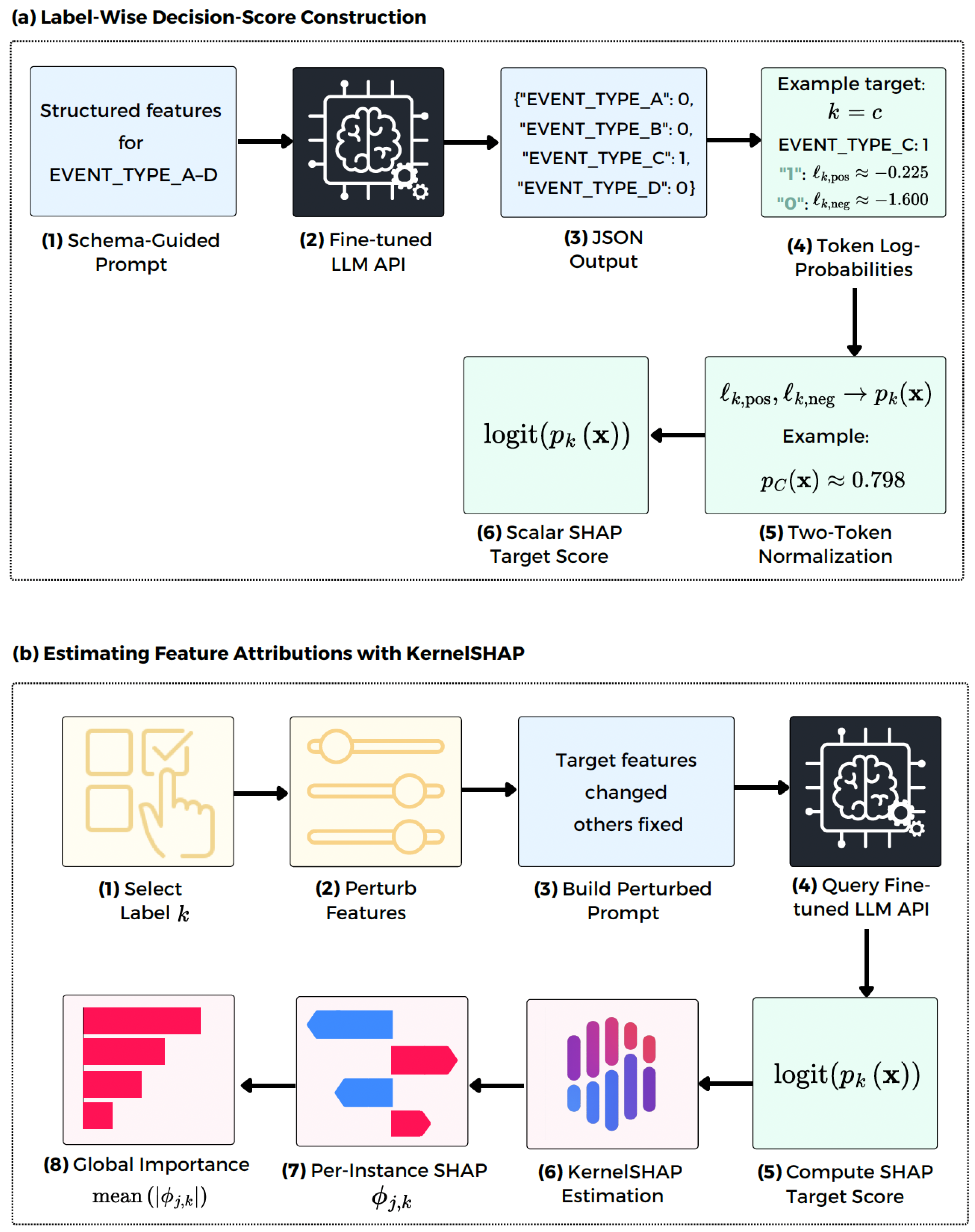
Each crime-type label is explained through a label-wise decision score derived from the decision-token log-probabilities. As summarized in Figure 6a, the schema-guided prompt is provided to the fine-tuned LLM through the API. The model returns structured JSON output, and the decision-token log-probabilities of “0” and “1” are normalized to obtain the label-wise decision score for the target label. KernelSHAP then perturbs the corresponding feature values through the schema-guided prompt and estimates feature attributions from the resulting changes in the target label score.

Label-Wise Decision-Score Construction

For each label k, we extract token log-probabilities for the possible values “0” (negative) and “1” (positive) at the position where the label value is generated in the JSON output [50,51]. Let ${𝓁}_{k,\mathrm{neg}}$ and ${𝓁}_{k,\mathrm{pos}}$ denote the corresponding log-probabilities. A positive class probability is then derived by exponentiating and normalizing over the two-token set:

$$p_k\left(\mathbf{x}\right)={\displaystyle \frac{exp\left({𝓁}_{k,\mathrm{pos}}\right)}{exp\left({𝓁}_{k,\mathrm{neg}}\right)+exp\left({𝓁}_{k,\mathrm{pos}}\right)}}.$$

(4)

$p_k\left(\mathbf{x}\right)$ is used as the label-wise decision score because it provides both a graded measure beyond the binary schema-guided JSON output and a stable scalar target for downstream attribution.

KernelSHAP Feature Attribution

Let k index the crime-type label being explained, and let $\mathbf{x}$ denote the corresponding label-specific input feature vector with d features. Using $p_k\left(\mathbf{x}\right)$ as the explained scalar function and setting link=“logit” in shap.KernelExplainer [52], the resulting SHAP attributions are additive in log-odds units:

$$logit\left(p_k\left(\mathbf{x}\right)\right)={\varphi }_{0,k}+{\displaystyle \sum _{j=1}^d}{\varphi }_{j,k}.$$

(5)

Here, j indexes the input features for label k, ${\varphi }_{j,k}$ denotes the contribution of feature j to the target crime-type score, and ${\varphi }_{0,k}$ is the corresponding base value. For each crime type, the full schema-guided prompt is reconstructed to preserve the same multi-label input structure used during fine-tuning. During a label-wise explanation run, only the event-specific feature values for the target crime type are perturbed, whereas the remaining event-type lines are kept fixed for the same (region_id, date) anchor. This procedure is illustrated in Figure 6b, where the selected label defines the target label-wise decision score, perturbed schema-guided prompts are repeatedly submitted through the fine-tuned LLM API, and KernelSHAP estimates per-instance feature attributions before aggregating them into global feature importance. Shared temporal indicators, such as day of week and month, are evaluated with respect to the same target label score. Thus, the resulting SHAP values describe feature contributions for the target crime type rather than for the bundled multi-label output as a whole.

KernelSHAP represents missing features using a background set $\mathcal{B}$ that approximates the input distribution [52]. To preserve chronological validity, $\mathcal{B}$ is constructed exclusively from the training split. Feature masking is implemented by replacing masked feature values in the serialized prompt with values drawn from $\mathcal{B}$ while retaining observed values for unmasked features. The exact background-set size and sampling settings are reported in Section 4. Explanations are computed separately for each label, and global importance is summarized by the mean absolute SHAP value per feature over the explained set.

3.4.2. Faithfulness Assessment Through Test-Time Feature Ablation

To complement the KernelSHAP analysis, a targeted test-time ablation is conducted to examine whether the feature ranked as most important also produces a measurable change in model behavior when its values are intervened on. The intervention is intentionally restricted to one feature per label because the goal is to assess the dominant attribution signal rather than to conduct an exhaustive ablation study. Model parameters remain fixed throughout; only selected input feature values are modified, while the prompt template and decoding setup are preserved.

For each label k, features are ranked using their global SHAP importance, computed as the mean absolute SHAP value over the explained set $\mathcal{T}$. The highest-ranked feature is selected as the ablation target for that label. A type-specific reference value ${\mu }_k$ is then computed as the training-set mean of the selected feature for crime type $c_k$. Thus, the ablation is applied label-wise: for each crime type $c_k$, the selected feature is replaced with its corresponding training-derived mean ${\mu }_k$ in the EVENT_TYPE_k line, while all other feature values remain unchanged. The same inference pipeline is then rerun. A consistent degradation after replacement is interpreted as evidence that anchor-level variation in the selected feature contributes to the model’s discrimination beyond its per-type average value. The ablation therefore serves as a behavioral faithfulness check that complements the SHAP attributions and helps assess whether the highly ranked feature reflects observable model reliance.

4. Experimental Setup

This section describes the experimental design used to evaluate the proposed framework. It outlines the datasets, compared models, training and inference settings, evaluation metrics, and explainability setup. The experiments assess predictive performance, cross-city performance, and post hoc feature attribution under schema-guided prediction conditions.

4.1. Datasets, Prediction Task, and Data Splits

The primary evaluation is conducted using NYC crime incident records derived from the NYPD Historic Complaint Data available through NYC Open Data [49]. Following prior crime prediction studies that use this public data source [36], the task is formulated as next-week crime occurrence prediction for four selected NYC crime types. The region–day panel, prediction anchors, labels, and engineered features follow the procedures described in Stages 1 and 2. For each region–day anchor, the objective is to predict whether at least one incident of each crime type occurs within the following seven-day window. The NYC experiment uses the leakage-safe chronological split defined in Stage 1. The training segment covers 1 January 2014 to 31 August 2015, the validation segment covers 1 September 2015 to 30 September 2015, and the test segment covers 1 October 2015 to 31 December 2015. After applying the anchor-retention and completeness criteria, the held-out NYC test split contains 19,750 anchors.

For supervised fine-tuning, a 30% stratified subsample of the NYC training anchors is used, resulting in 45,076 SFT training anchors. The validation split contains 5750 anchors and is used for validation-based monitoring and model selection, while the held-out test split is reserved for final performance reporting.

In addition to the NYC evaluation, Chicago is used as an external test-only setting for cross-city evaluation. The Chicago incident records are derived from the City of Chicago crime data portal [64], which has also been used in prior crime prediction benchmarks [36]. The Chicago region–day anchors are generated using the same preprocessing, feature engineering, and prompt-generation procedures applied in this study. After applying the same anchor-retention and completeness criteria, the final Chicago evaluation contains 15,326 region–day anchors. The Chicago data are not used during training, validation, fine-tuning, or model selection. The base GPT-4.1-mini and XCrime-LLM are applied directly to the Chicago test data using the same prediction horizon and evaluation metrics. For the NYC evaluation, the abstract event-type identifiers EVENT_TYPE_A–EVENT_TYPE_D correspond, in order, to Burglary, Robbery, Grand Larceny, and Felony Assault. For the Chicago evaluation, the same identifiers are reused but mapped, in order, to Theft, Battery, Criminal Damage, and Assault.

4.2. Model Comparison, Training, and Inference Settings

Five prediction approaches are evaluated under a common experimental setup: zero-shot GPT-4.1-mini, few-shot GPT-4.1-mini, XCrime-LLM, XGBoost, and MLP. The zero-shot and few-shot GPT-4.1-mini are evaluated as prompting baselines. In these settings, the model weights are not updated; only the inference time prompt changes. The zero-shot baseline uses the schema-guided prompt without exemplars, whereas the few-shot baseline adds three fixed exemplars from the training split to maintain a consistent prompting context across all test instances. Both prompting baselines are assessed directly on the held-out test split to measure performance without supervised fine-tuning. Key training, inference, validation, and stopping settings for the compared prediction approaches are summarized in

Table 5. Training, inference, and validation settings for the compared models.

Model	Key Settings	Validation/Stopping
GPT-4.1-mini (zero-shot)	Temperature = 0 top-p = 1 Schema-guided prompt and JSON output Schema validation	No parameter training or validation-based stopping; evaluated on the test split.
GPT-4.1-mini (few-shot)	Three fixed exemplars from the training split Temperature = 0 top-p = 1 Schema-guided prompt and JSON output Schema validation	No parameter training or validation-based stopping; evaluated on the test split.
XCrime-LLM	Fine-tuned from gpt-4.1-mini-2025-04-14 Temperature = 0 top-p = 1 Schema-guided prompt and JSON output Schema validation	Validation split used during fine-tuning; final evaluation on the test split.
XGBoost (one-vs.-rest)	Binary logistic objective 1000 trees Learning rate = 0.03 Max depth = 5 Subsample = 0.8 Colsample = 0.8 Seed = 42 Decision threshold = 0.5	Early stopping on validation log loss (patience = 80).
MLP	Hidden layers (256, 128) Dropout = 0.2 BCEWithLogitsLoss AdamW optimizer Learning rate = ${10}^{-3}$ Batch size = 256 Decision threshold = 0.5	Up to 50 epochs; early stopping on validation micro-F1 (patience = 7); best checkpoint retained.

. These settings clarify how the LLM prompting baselines, the fine-tuned GPT-4.1-mini predictor used in XCrime-LLM, and the trained non-LLM baselines are evaluated under the same data splits, prediction task, and evaluation metrics.

4.3. Evaluation Metrics

Final performance is reported on the held-out test split using Micro-F1 and Macro-F1 as the primary evaluation metrics. For selected trained models, per-crime-type precision, recall, and F1-score are also reported to provide a label-wise view of model behavior. Micro-F1 reflects overall performance across all labels, whereas Macro-F1 gives equal weight to each crime type.

For an evaluation set with K labels (here, K = 4), let ${\mathrm{TP}}_k$, ${\mathrm{FP}}_k$, and ${\mathrm{FN}}_k$ denote the true-positive, false-positive, and false-negative counts for label k, respectively.

Micro-F1 is defined as

$$\mathrm{F}{1}_{\mathrm{micro}}={\displaystyle \frac{2·{\mathrm{Precision}}_{\mathrm{micro}}·{\mathrm{Recall}}_{\mathrm{micro}}}{{\mathrm{Precision}}_{\mathrm{micro}}+{\mathrm{Recall}}_{\mathrm{micro}}}},$$

(6)

where

$${\mathrm{Precision}}_{\mathrm{micro}}={\displaystyle \frac{{\sum }_k{\mathrm{TP}}_k}{{\sum }_k({\mathrm{TP}}_k+{\mathrm{FP}}_k)}},{\mathrm{Recall}}_{\mathrm{micro}}={\displaystyle \frac{{\sum }_k{\mathrm{TP}}_k}{{\sum }_k({\mathrm{TP}}_k+{\mathrm{FN}}_k)}}.$$

(7)

Macro-F1 is defined as

$$\mathrm{F}{1}_{\mathrm{macro}}={\displaystyle \frac{1}{K}}{\displaystyle \sum _{k=1}^K}{\displaystyle \frac{2·{\mathrm{Precision}}_k·{\mathrm{Recall}}_k}{{\mathrm{Precision}}_k+{\mathrm{Recall}}_k}},$$

(8)

where

$${\mathrm{Precision}}_k={\displaystyle \frac{{\mathrm{TP}}_k}{{\mathrm{TP}}_k+{\mathrm{FP}}_k}},{\mathrm{Recall}}_k={\displaystyle \frac{{\mathrm{TP}}_k}{{\mathrm{TP}}_k+{\mathrm{FN}}_k}}.$$

(9)

4.4. Explainability and Faithfulness Evaluation

Explainability analysis is conducted separately for each crime-type label using KernelSHAP under API-only black-box access. For label k, only the corresponding event-type line is modified during explanation, whereas the remaining event-type lines are kept fixed at their observed values for the same (region_id, date) anchor. Faithfulness is assessed through targeted test-time ablation by replacing the top-ranked feature for each label with the corresponding training-set mean ${\mu }_k$. The main settings for the explainability and faithfulness evaluation are summarized in

Table 6. Setup for explainability and faithfulness analysis.

Setting	Value
Explanation method	KernelSHAP
Explained scalar	Label-wise decision score derived from decision-token log-probabilities
Background set	Training split only, $\left|\mathcal{B}\right|=15$ per label
Explained set	Held-out test split, $\left|\mathcal{T}\right|=50$ per label
Random seed	42
SHAP samples per instance	32
Perturbation scope	Label-specific feature line is varied while other crime-type lines are fixed
Global importance summary	Mean absolute SHAP value
Faithfulness test	Targeted test-time ablation
Ablated feature	Top-ranked feature for each label based on global SHAP importance
Replacement value	Crime-type-specific training-set mean ${\mu }_k$

, including the label-wise decision score, KernelSHAP sampling configuration, perturbation scope, global feature importance summary, and targeted test-time ablation rule.

5. Results and Discussion

This section presents the experimental results and discusses the predictive performance, cross-city behavior, and explainability of the proposed XCrime-LLM framework. First, XCrime-LLM is evaluated on the NYC test split and compared with zero-shot and few-shot GPT-4.1-mini, XGBoost, and MLP baselines. Second, a cross-city evaluation is conducted on the Chicago dataset. Finally, KernelSHAP and targeted test-time ablation are used to analyze feature reliance and assess whether the explanation results are reflected in observable model behavior.

5.1. Overall Predictive Performance

Following the task definition and leakage-safe split protocol described in Section 3.1, the primary evaluation examines next-week crime occurrence prediction on the NYC test split for four crime types: Burglary, Robbery, Felony Assault, and Grand Larceny.

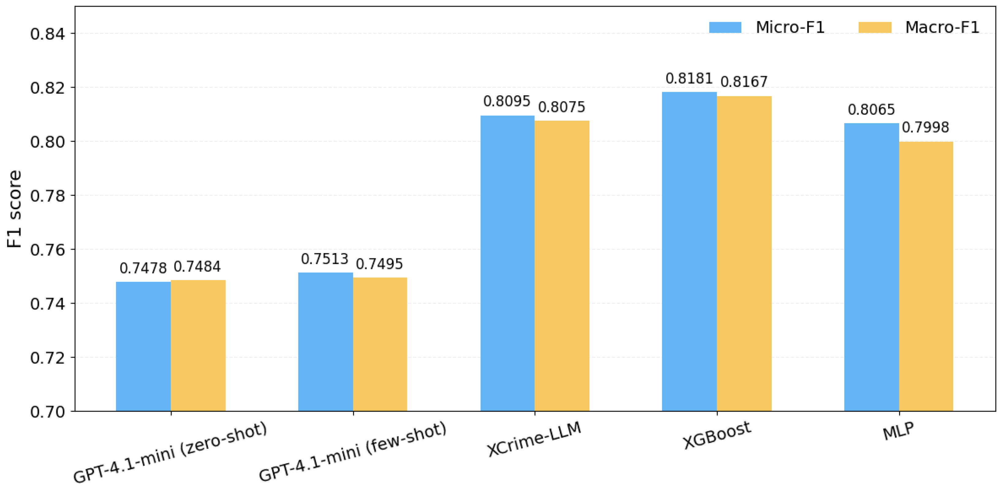
In this subsection, XCrime-LLM denotes the proposed framework instantiated with the fine-tuned GPT-4.1-mini, whereas zero-shot and few-shot GPT-4.1-mini are treated as prompting baselines. The comparison is made under the same schema-guided prompting setup and schema-guided JSON output format. The overall multi-label results are summarized in Figure 7, and per-crime-type precision, recall, and F1-score for the top-performing trained models are reported in

Table 7. Per-crime-type precision, recall, and F1-score on the NYC test split.

Crime Type	XCrime-LLM			XGBoost			MLP
	Precision	Recall	F1	Precision	Recall	F1	Precision	Recall	F1
Burglary	0.7758	0.7570	0.7663	0.7877	0.7692	0.7783	0.7914	0.7390	0.7643
Robbery	0.8155	0.7948	0.8050	0.8178	0.7941	0.8058	0.8255	0.7691	0.7963
Grand Larceny	0.8644	0.8637	0.8640	0.8647	0.8859	0.8752	0.8587	0.8655	0.8621
Felony Assault	0.7883	0.8012	0.7947	0.7917	0.8239	0.8075	0.8034	0.7513	0.7765

Note: Bold values indicate the highest score for each crime type and metric across the compared models.

.

Supervised fine-tuning improves predictive performance over zero-shot GPT-4.1-mini, with Micro-F1 increasing from 0.7478 to 0.8095 and Macro-F1 from 0.7484 to 0.8075. The zero-shot and few-shot settings differ only in the use of fixed in-context examples, whereas supervised fine-tuning adapts the base GPT-4.1-mini using task-specific prompt–output pairs from the training anchors. Because all LLM settings use the same schema-guided prompting and JSON output format, the observed gain is mainly associated with task-specific fine-tuning rather than a different input or output interface.

Few-shot GPT-4.1-mini provides only a marginal improvement over zero-shot and remains clearly below XCrime-LLM, indicating that a small number of in-context examples is insufficient to match the task adaptation achieved through fine-tuning.

Across the per-crime-type results, XGBoost achieves the highest F1-scores, while XCrime-LLM remains competitive across the evaluated labels. This result is consistent with the task being based on engineered tabular spatio-temporal features, a setting in which gradient-boosted trees are often strong performers. The strong XGBoost result also supports the usefulness of the proposed feature representation, since this baseline uses the same engineered inputs. Within this feature setting, the competitive performance of XCrime-LLM indicates that the fine-tuned LLM can learn from structured spatio-temporal inputs while retaining the schema-guided interface used in the proposed framework.

Overall, supervised fine-tuning provides a clear gain over prompting baselines, while XCrime-LLM remains close to the trained tabular baselines under the same engineered feature setting.

5.2. Cross-City Transfer

To examine cross-city transfer beyond the training city, an additional evaluation is conducted on the Chicago dataset using the same experimental framework described in Section 4. The data construction and preprocessing steps are reapplied to Chicago-specific coordinates, region definitions, and corresponding crime types. In this setting, the abstract event-type labels are mapped to Chicago-specific crime types rather than to the NYC crime types used in the main experiment. Specifically, EVENT_TYPE_A–EVENT_TYPE_D are mapped, in order, to Theft, Battery, Criminal Damage, and Assault. In this transfer setting, the base GPT-4.1-mini is evaluated using the same schema-guided prompting format, while XCrime-LLM uses the GPT-4.1-mini model fine-tuned only on NYC training anchors. Thus, the Chicago evaluation examines transfer under the shared prediction interface rather than adaptation to Chicago-specific training data.

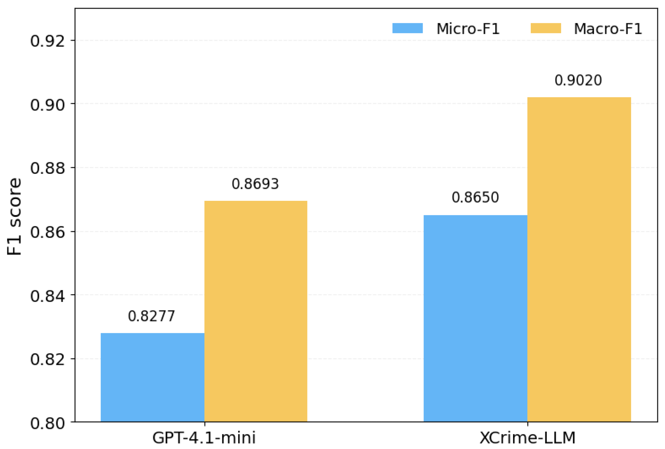
Accordingly, the Chicago results should not be interpreted as a direct comparison of identical named crime categories across NYC and Chicago. Despite this stricter transfer setting, XCrime-LLM outperforms the non-fine-tuned GPT-4.1-mini, improving Micro-F1 from 0.8277 to 0.8650 and Macro-F1 from 0.8693 to 0.9020.

The overall Chicago transfer results are summarized in Figure 8, which compares the overall Micro-F1 and Macro-F1 scores of the base GPT-4.1-mini and XCrime-LLM in the same Chicago cross-city evaluation setting.

Table 8. Per-crime-type Chicago transfer performance.

Crime Type	Base GPT-4.1-mini			XCrime-LLM
	Precision	Recall	F1	Precision	Recall	F1
Theft	0.9028	0.9141	0.9084	0.9411	0.9147	0.9277
Battery	0.9054	0.9093	0.9073	0.9493	0.8951	0.9214
Criminal Damage	0.8635	0.8599	0.8617	0.8478	0.9526	0.8972
Assault	0.8056	0.7942	0.7999	0.7933	0.9427	0.8616

Note: Bold values indicate the highest score for each crime type and metric across the compared models.

reports the per-crime-type precision, recall, and F1-score for the two models.

At the label level, XCrime-LLM improves the F1-score for all four mapped Chicago crime types, although the balance between precision and recall differs across labels.

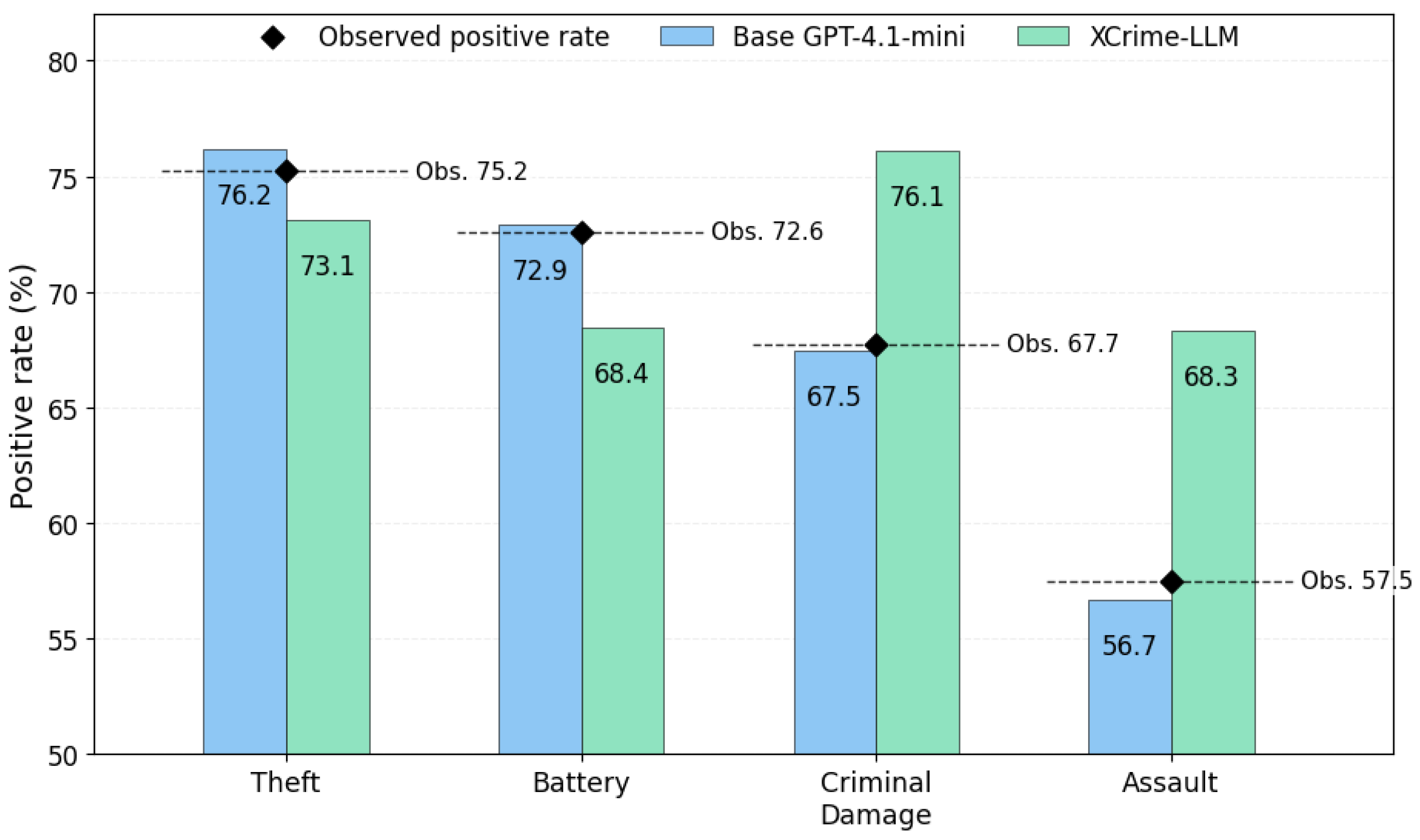
As shown in Figure 9, the predicted-positive rates help explain these label-wise differences. For Theft and Battery, XCrime-LLM improves F1 while reducing the predicted-positive rate relative to the non-fine-tuned GPT-4.1-mini, suggesting a more selective prediction pattern. In contrast, for Criminal Damage and Assault, XCrime-LLM increases recall and F1, but this improvement is accompanied by a predicted-positive rate above the observed positive rate. This indicates that part of the transfer gain comes from a stronger tendency to predict the positive class for these labels.

These results suggest that XCrime-LLM retains useful predictive behavior when applied to Chicago under the shared schema-guided interface, while still showing label-wise calibration differences in the transfer setting. Because the abstract event-type labels are mapped to city-specific crime categories, the observed gains should be interpreted as transfer under the shared prediction interface rather than direct equivalence between identical named crime categories across cities.

5.3. Global Feature Importance

To better understand the decision behavior of XCrime-LLM, we analyze global feature importance using KernelSHAP. The explainability analysis focuses on XCrime-LLM because the framework is designed to support explanation under black-box API access, where internal model parameters and model-internal feature-importance mechanisms are not available.

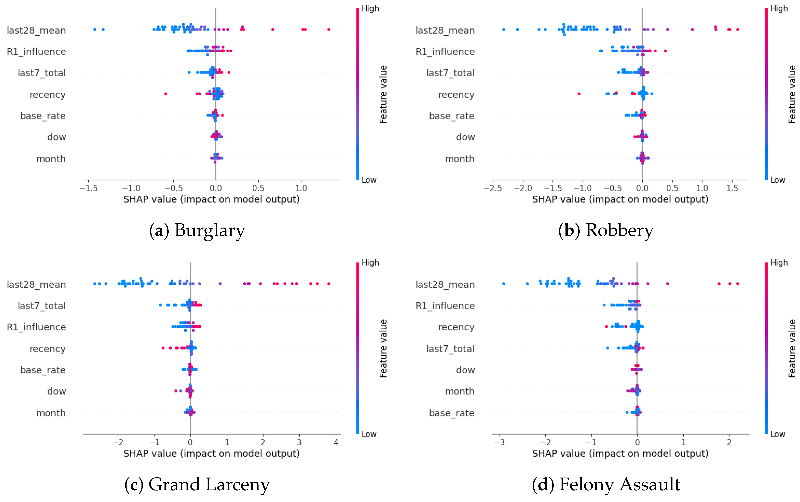
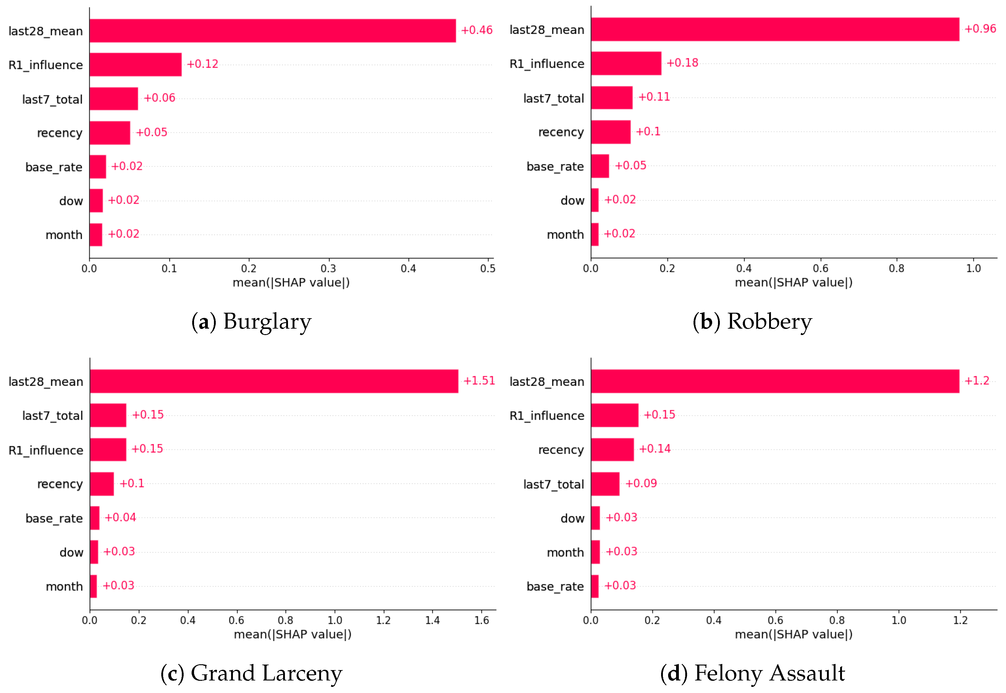
KernelSHAP attributions are computed separately for each crime type to identify which engineered inputs most strongly influence the label-wise decision scores. Figure 10 summarizes the mean absolute SHAP values, which provide the global feature-importance ranking for each crime type. In these bar plots, longer bars indicate features with larger mean absolute feature attribution values across the explained test instances. Because these values are based on |SHAP|, they reflect the magnitude of each feature’s contribution rather than the direction of its effect. Across all four crime types, last28_mean has the highest mean |SHAP| value, indicating that the mean crime level over the previous 28 days receives the strongest global attribution. Secondary contributions are observed for R1_influence, last7_total, and recency, whereas base_rate, dow, and month show comparatively small global importance.

The beeswarm plots in Figure 11 complement the mean |SHAP| rankings by showing both the direction and spread of feature effects. Each point represents an explained test instance, with positive SHAP values increasing the label-wise decision score and negative SHAP values decreasing it. The color of each point indicates the corresponding feature value, allowing the plots to show whether low or high feature values are associated with positive or negative feature attributions. Across all four crime types, last28_mean shows the widest horizontal spread and the clearest directional pattern: low values are mostly associated with negative SHAP values, whereas high values are associated with positive SHAP values. This indicates that medium-term historical intensity has a consistent positive association with the label-wise decision scores. The remaining features are more concentrated around zero, indicating smaller and more label-specific effects.

Given this strong and consistent attribution, we next perform a targeted test-time ablation to assess whether the SHAP ranking is reflected in the model’s predictive behavior.

5.4. Targeted Test-Time Ablation

To assess whether the KernelSHAP explanations reflect the model’s observable decision behavior, we perform a targeted test-time ablation of last28_mean, the feature identified as most influential across all crime types. Specifically, the ablation tests whether removing the anchor-specific information carried by last28_mean changes predictive performance in a way that is consistent with its high SHAP importance.

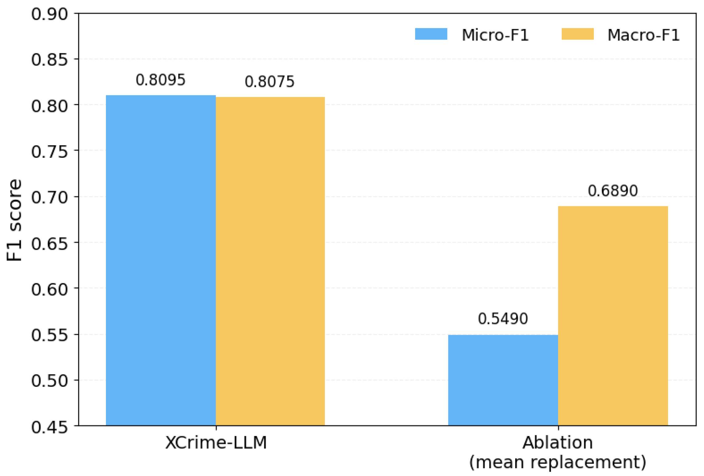
The model and inference setup are held fixed; only last28_mean is replaced with the corresponding training-set mean ${\mu }_k$ for crime type $c_k$. All other features remain unchanged. This intervention removes anchor-level variation in last28_mean while replacing it with a typical training-set value for each crime type. As shown in Figure 12, this single-feature replacement produces a substantial performance degradation: Micro-F1 drops from 0.8095 to 0.5490 and Macro-F1 from 0.8075 to 0.6890. The larger drop in Micro-F1 indicates that the ablation affects the model’s overall multi-label decision behavior, while the decrease in Macro-F1 suggests that the effect is also reflected across crime types rather than being limited to a single label. This drop provides initial evidence that last28_mean is behaviorally influential in the model’s predictions.

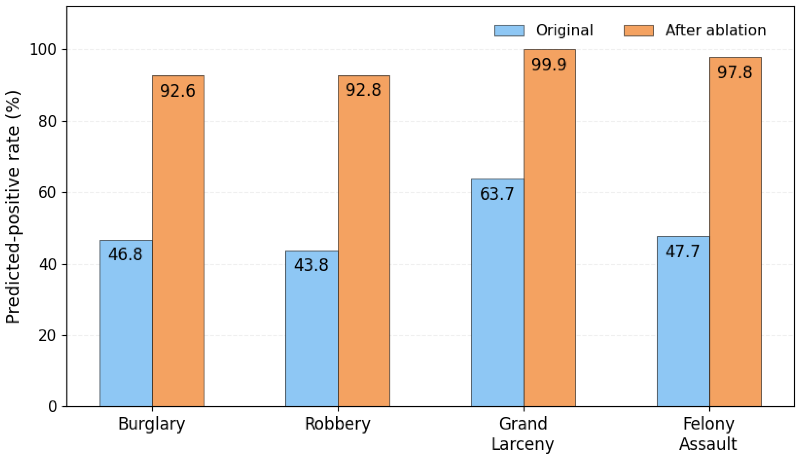
The ablation changes the model’s decision behavior in a clear and consistent pattern. As shown in Figure 13, replacing last28_mean sharply increases the predicted-positive rate across crime types, indicating that the model predicts the positive class for a much larger share of anchors. The increase is especially pronounced for Burglary, Robbery, and Felony Assault, where the predicted-positive rates rise from below 50% in the original setting to above 90% after ablation. This shift is also reflected in the per-crime-type metrics reported in

Table 9. Per-crime-type effect of last28_mean ablation on XCrime-LLM performance.

Crime Type	Original			After Ablation
	Precision	Recall	F1	Precision	Recall	F1
Burglary	0.7758	0.7570	0.7663	0.5138	0.9929	0.6772
Robbery	0.8155	0.7948	0.8050	0.4841	0.9994	0.6523
Grand Larceny	0.8644	0.8637	0.8640	0.6382	0.9998	0.7791
Felony Assault	0.7883	0.8012	0.7947	0.4792	0.9984	0.6476

: recall increases to near-perfect levels, but precision drops substantially, resulting in lower F1-scores across all crime types. This pattern suggests that, without anchor-level variation in last28_mean, the model becomes less able to separate positive from negative cases and instead shifts toward overpredicting the positive label.

Taken together, the ablation results show that XCrime-LLM relies strongly on anchor-level variation in last28_mean as a discriminative signal, rather than merely using its per-crime-type average value. This finding supports the SHAP analysis, because the feature with the strongest global attribution also produces a clear degradation in predictive behavior when its instance-level variation is removed. At the same time, the large performance drop indicates sensitivity to this feature, highlighting the importance of monitoring medium-term historical intensity when interpreting and applying the model’s predictions.

6. Conclusions and Future Work

This study presents and evaluates XCrime-LLM for next-week crime occurrence prediction under API-only black-box access. On the NYC test split, XCrime-LLM outperformed the prompting baselines and remained competitive with the trained non-LLM baselines, although XGBoost achieved the best overall scores in this structured feature-based setting. In a cross-city evaluation using Chicago data, XCrime-LLM also outperformed the base GPT-4.1-mini without further fine-tuning or adaptation, suggesting useful cross-city predictive behavior under the shared schema-guided prediction interface while also revealing label-wise calibration differences.

To examine explainability under black-box constraints, KernelSHAP was used to analyze label-wise feature importance in XCrime-LLM. Across all crime types, last28_mean emerged as the dominant feature, with higher medium-term historical intensity generally increasing the label-wise decision score. To assess whether these feature attributions were reflected in observable model behavior, a targeted test-time ablation replaced last28_mean with the corresponding training-set mean for each crime type. This intervention caused a substantial drop in both Micro-F1 and Macro-F1 and shifted the model toward overpredicting the positive label. Together, the KernelSHAP and ablation results provide complementary evidence that last28_mean is both highly ranked by the explanation method and behaviorally influential.

Future work should extend the evaluation to additional cities and broader temporal settings to examine the generality of the observed transfer behavior. In particular, city-specific fine-tuning and threshold optimization may help improve label-level decision balance and calibration in external evaluation settings. Enriching the feature set with external signals such as mobility patterns, weather, and special events may also be promising. The dominance of last28_mean suggests that richer contextual signals could help improve prediction beyond medium-term historical intensity alone. It would also be valuable to extend the current next-week formulation to multiple prediction horizons, including 1-day and 14-day settings, to examine whether the predictive patterns observed in this study remain stable across different horizons.

Overall, this study highlights the value of an explainable, schema-guided LLM framework for spatio-temporal crime prediction under black-box API constraints, offering a foundation for decision support applications that require structured outputs and post hoc feature attribution.

References

- Raj, P.; Kalluru, S.R. Does crime impede economic growth? An evidence from India. Cogent Soc. Sci. 2023, 9, 2196814. [Google Scholar] [CrossRef] [Scilit]
- McCollister, K.E.; French, M.T.; Fang, H. The cost of crime to society: New crime-specific estimates for policy and program evaluation. Drug Alcohol Depend. 2010, 108, 98–109. [Google Scholar] [CrossRef] [Scilit] [PubMed]
- Bureau of Justice Statistics. Costs of Crime. U.S. Department of Justice. 2022. Available online: https://bjs.ojp.gov/topics/costs-crime (accessed on 25 January 2026).
- Anderson, D.A. The aggregate cost of crime in the United States. J. Law Econ. 2021, 64, 857–885. [Google Scholar] [CrossRef] [Scilit] [PubMed]
- Domínguez, P.; Scartascini, C. Willingness to pay for crime reduction: The role of information in the Americas. J. Public Econ. 2024, 239, 105205. [Google Scholar] [CrossRef] [Scilit]
- Weisburd, D. The Law of Crime Concentration and the Criminology of Place. Criminology 2015, 53, 133–157. [Google Scholar] [CrossRef] [Scilit]
- Du, Y.; Ding, N. A systematic review of multi-scale spatio-temporal crime prediction methods. ISPRS Int. J. Geo-Inf. 2023, 12, 209. [Google Scholar] [CrossRef] [Scilit]
- Almuhanna, A.A.; Alrehili, M.M.; Alsubhi, S.H.; Syed, L. Prediction of crime in neighbourhoods of New York City using spatial data analysis. In 2021 1st International Conference on Artificial Intelligence and Data Analytics (CAIDA); IEEE: Piscataway, NJ, USA, 2021; pp. 23–30. [Google Scholar] [CrossRef] [Scilit]
- Mandalapu, V.; Elluri, L.; Vyas, P.; Roy, N. Crime prediction using machine learning and deep learning: A systematic review and future directions. IEEE Access 2023, 11, 60153–60170. [Google Scholar] [CrossRef] [Scilit]
- Huang, C.; Zhang, J.; Zheng, Y.; Chawla, N.V. DeepCrime: Attentive hierarchical recurrent networks for crime prediction. In Proceedings of the 27th ACM International Conference on Information and Knowledge Management; Association for Computing Machinery: New York, NY, USA, 2018; pp. 1423–1432. [Google Scholar] [CrossRef] [Scilit]
- Han, Y.; Hu, Y.; Zhu, H.; Wang, F. A cyclically adjusted spatio-temporal kernel density estimation method for predictive crime hotspot analysis. Ann. GIS 2023, 29, 177–191. [Google Scholar] [CrossRef] [Scilit]
- Arrieta, A.B.; Díaz-Rodríguez, N.; Del Ser, J.; Bennetot, A.; Tabik, S.; Barbado, A.; García, S.; Gil-López, S.; Molina, D.; Benjamins, R.; et al. Explainable Artificial Intelligence (XAI): Concepts, taxonomies, opportunities and challenges toward responsible AI. Inf. Fusion 2020, 58, 82–115. [Google Scholar] [CrossRef] [Scilit]
- Rudin, C. Stop Explaining Black Box Machine Learning Models for High Stakes Decisions and Use Interpretable Models Instead. Nat. Mach. Intell. 2019, 1, 206–215. [Google Scholar] [CrossRef] [Scilit] [PubMed]
- Ersöz, F.; Ersöz, T.; Marcelloni, F.; Ruffini, F. Artificial Intelligence in Crime Prediction: A Survey with a Focus on Explainability. IEEE Access 2025, 13, 59646–59674. [Google Scholar] [CrossRef] [Scilit]
- Guidotti, R.; Monreale, A.; Ruggieri, S.; Turini, F.; Giannotti, F.; Pedreschi, D. A Survey of Methods for Explaining Black Box Models. ACM Comput. Surv. 2018, 51, 1–42. [Google Scholar] [CrossRef] [Scilit]
- Ribeiro, M.T.; Singh, S.; Guestrin, C. Why Should I Trust You? Explaining the Predictions of Any Classifier. In Proceedings of the 22nd ACM SIGKDD International Conference on Knowledge Discovery and Data Mining; Association for Computing Machinery: New York, NY, USA, 2016; pp. 1135–1144. [Google Scholar] [CrossRef] [Scilit]
- Lundberg, S.M.; Lee, S.I. A Unified Approach to Interpreting Model Predictions. In NIPS’17: Proceedings of the 31st International Conference on Neural Information Processing Systems; Advances in Neural Information Processing Systems; Curran Associates Inc.: Red Hook, NY, USA, 2017; Volume 30. [Google Scholar]
- Brown, T.B.; Mann, B.; Ryder, N.; Subbiah, M.; Kaplan, J.D.; Dhariwal, P.; Neelakantan, A.; Shyam, P.; Sastry, G.; Askell, A.; et al. Language Models Are Few-Shot Learners. In NIPS’20: Proceedings of the 34th International Conference on Neural Information Processing Systems; Advances in Neural Information Processing Systems; Curran Associates Inc.: Red Hook, NY, USA, 2020; Volume 33, pp. 1877–1901. [Google Scholar]
- Ouyang, L.; Wu, J.; Jiang, X.; Almeida, D.; Wainwright, C.; Mishkin, P.; Zhang, C.; Agarwal, S.; Slama, K.; Ray, A.; et al. Training Language Models to Follow Instructions with Human Feedback. In NIPS’22: Proceedings of the 36th International Conference on Neural Information Processing Systems; Advances in Neural Information Processing Systems; Curran Associates Inc.: Red Hook, NY, USA, 2022; Volume 35, pp. 27730–27744. [Google Scholar]
- Hegselmann, S.; Buendia, A.; Lang, H.; Agrawal, M.; Jiang, X.; Sontag, D. TabLLM: Few-shot Classification of Tabular Data with Large Language Models. In Proceedings of the Proceedings of The 26th International Conference on Artificial Intelligence and Statistics; Proceedings of Machine Learning Research; PMLR: Cambridge, MA, USA, 2023; Volume 206, pp. 5549–5581. [Google Scholar]
- Jaitly, S.; Shah, T.; Shugani, A.; Grewal, R.S. Towards Better Serialization of Tabular Data for Few-shot Classification with Large Language Models. arXiv 2023, arXiv:2312.12464. [Google Scholar] [CrossRef] [Scilit]
- Fang, X.; Xu, W.; Tan, F.A.; Hu, Z.; Zhang, J.; Qi, Y.; Sengamedu, S.H.; Faloutsos, C. Large Language Models (LLMs) on Tabular Data: Prediction, Generation, and Understanding—A Survey. Trans. Mach. Learn. Res. 2024. Available online: https://openreview.net/forum?id=IZnrCGF9WI (accessed on 10 May 2026).
- Li, Z.; Xia, L.; Tang, J.; Xu, Y.; Shi, L.; Xia, L.; Yin, D.; Huang, C. UrbanGPT: Spatio-Temporal Large Language Models. In Proceedings of the 30th ACM SIGKDD Conference on Knowledge Discovery and Data Mining; Association for Computing Machinery: New York, NY, USA, 2024; pp. 5351–5362. [Google Scholar] [CrossRef] [Scilit]
- Sarzaeim, P.; Mahmoud, Q.H.; Azim, A. A Framework for LLM-Assisted Smart Policing System. IEEE Access 2024, 12, 74915–74929. [Google Scholar] [CrossRef] [Scilit]
- He, Z.; Tao, L.; Xie, Z.; Xu, C. Discovering spatial interaction patterns of near repeat crime by spatial association rules mining. Sci. Rep. 2020, 10, 17262. [Google Scholar] [CrossRef] [Scilit]
- Mytheli, R.; Subha, A.; Sivakumar, T. Crime Prediction and Pattern Analysis Using Machine Learning Techniques. Int. J. Sci. Res. Sci. Technol. 2025, 12, 638–648. [Google Scholar] [CrossRef] [Scilit]
- Kshatri, S.S.; Singh, D.; Narain, B.; Bhatia, S.; Quasim, M.T.; Sinha, G.R. An empirical analysis of machine learning algorithms for crime prediction using stacked generalization: An ensemble approach. IEEE Access 2021, 9, 67488–67500. [Google Scholar] [CrossRef] [Scilit]
- Wu, X.; Huang, C.; Zhang, C.; Chawla, N.V. Hierarchically Structured Transformer Networks for Fine-Grained Spatial Event Forecasting. In Proceedings of the Web Conference 2020; Association for Computing Machinery: New York, NY, USA, 2020; pp. 2320–2330. [Google Scholar] [CrossRef] [Scilit]
- Vaswani, A.; Shazeer, N.; Parmar, N.; Uszkoreit, J.; Jones, L.; Gomez, A.N.; Kaiser, Ł.; Polosukhin, I. Attention Is All You Need. In NIPS’17: Proceedings of the 31st International Conference on Neural Information Processing Systems; Advances in Neural Information Processing Systems; Curran Associates Inc.: Red Hook, NY, USA, 2017; Volume 30. [Google Scholar]
- Zhou, J.; Cui, G.; Hu, S.; Zhang, Z.; Yang, C.; Liu, Z.; Wang, L.; Li, C.; Sun, M. Graph neural networks: A review of methods and applications. AI Open 2020, 1, 57–81. [Google Scholar] [CrossRef] [Scilit]
- Rayhan, Y.; Hashem, T. AIST: An Interpretable Attention-Based Deep Learning Model for Crime Prediction. In ACM Transactions on Spatial Algorithms and Systems; Association for Computing Machinery: New York, NY, USA, 2023; Volume 9, pp. 1–31. [Google Scholar] [CrossRef] [Scilit]
- Sun, M.; Zhou, P.; Tian, H.; Liao, Y.; Xie, H. Spatial-Temporal Attention Network for Crime Prediction with Adaptive Graph Learning. In Proceedings of the International Conference on Artificial Neural Networks; Springer: Cham, Switzerland, 2022; pp. 656–669. [Google Scholar] [CrossRef] [Scilit]
- Jain, S.; Wallace, B.C. Attention is not Explanation. In Proceedings of the 2019 Conference of the North American Chapter of the Association for Computational Linguistics: Human Language Technologies, Volume 1 (Long and Short Papers); Association for Computational Linguistics: Stroudsburg, PA, USA, 2019; pp. 3543–3556. [Google Scholar] [CrossRef] [Scilit]
- Serrano, S.; Smith, N.A. Is Attention Interpretable? In Proceedings of the 57th Annual Meeting of the Association for Computational Linguistics; Association for Computational Linguistics: Stroudsburg, PA, USA, 2019; pp. 2931–2951. [Google Scholar] [CrossRef] [Scilit]
- Xia, L.; Huang, C.; Xu, Y.; Dai, P.; Bo, L.; Zhang, X.; Chen, T. Spatial-Temporal Sequential Hypergraph Network for Crime Prediction with Dynamic Multiplex Relation Learning. In Proceedings of the Thirtieth International Joint Conference on Artificial Intelligence, IJCAI-21; International Joint Conferences on Artificial Intelligence Organization: Marina del Rey, CA, USA, 2021; pp. 1631–1637. [Google Scholar] [CrossRef] [Scilit]
- Li, Z.; Huang, C.; Xia, L.; Xu, Y.; Pei, J. Spatial-Temporal Hypergraph Self-Supervised Learning for Crime Prediction. In 2022 IEEE 38th International Conference on Data Engineering (ICDE); IEEE: Piscataway, NJ, USA, 2022; pp. 2984–2996. [Google Scholar] [CrossRef] [Scilit]
- Liang, K.; Zhou, S.; Liu, M.; Liu, Y.; Tu, W.; Zhang, Y.; Fang, L.; Liu, Z.; Liu, X. Hawkes-Enhanced Spatial-Temporal Hypergraph Contrastive Learning Based on Criminal Correlations. In Proceedings of the AAAI Conference on Artificial Intelligence; Association for the Advancement of Artificial Intelligence: Washington, DC, USA, 2024; Volume 38, pp. 8733–8741. [Google Scholar] [CrossRef] [Scilit]
- Tang, J.; Xia, L.; Huang, C. Explainable spatio-temporal graph neural networks. In Proceedings of the 32nd ACM International Conference on Information and Knowledge Management; Association for Computing Machinery: New York, NY, USA, 2023; pp. 2432–2441. [Google Scholar] [CrossRef] [Scilit]
- Adebayo, J.; Gilmer, J.; Muelly, M.; Goodfellow, I.; Hardt, M.; Kim, B. Sanity Checks for Saliency Maps. In Proceedings of the Advances in Neural Information Processing Systems; Curran Associates Inc.: Red Hook, NY, USA, 2018; Volume 31. [Google Scholar]
- Yeh, C.K.; Hsieh, C.Y.; Suggala, A.; Inouye, D.I.; Ravikumar, P.K. On the (In)fidelity and Sensitivity of Explanations. In Proceedings of the 33rd International Conference on Neural Information Processing Systems; Advances in Neural Information Processing Systems; Curran Associates Inc.: Red Hook, NY, USA, 2019; Volume 32, pp. 10967–10978. [Google Scholar]
- Hooker, S.; Erhan, D.; Kindermans, P.J.; Kim, B. A Benchmark for Interpretability Methods in Deep Neural Networks. In Proceedings of the 33rd International Conference on Neural Information Processing Systems; Proceedings of the Advances in Neural Information Processing Systems; Curran Associates Inc.: Red Hook, NY, USA, 2019; Volume 32. [Google Scholar]
- Sun, T.; Shao, Y.; Qian, H.; Huang, X.; Qiu, X. Black-Box Tuning for Language-Model-as-a-Service. In Proceedings of the 39th International Conference on Machine Learning; PMLR: Cambridge, MA, USA, 2022; Volume 162, pp. 20841–20855. [Google Scholar]
- Acampora, G.; Vitiello, A. Local Interpretable Model-agnostic Explanations for Crime Prediction. In 2025 IEEE Symposium on Trustworthy, Explainable and Responsible Computational Intelligence (CITREx Companion); IEEE: Piscataway, NJ, USA, 2025; pp. 1–4. [Google Scholar] [CrossRef] [Scilit]
- Kim, G.; Cho, Y.; Han, Y.; Lee, G. Crime Mapping in Urban Environments Using Explainable AI: A Case Study of Daegu, Korea. Sustain. Cities Soc. 2025, 130, 106507. [Google Scholar] [CrossRef] [Scilit]
- Chen, T.; Bowers, K.; Cheng, T. The impacts of specific place visitations on theft patterns: A case study in Greater London, UK. Comput. Urban Sci. 2025, 5, 30. [Google Scholar] [CrossRef] [Scilit]
- Khalfa, R.; Theinert, N.; Hardyns, W. Comparing XAI techniques for interpreting short-term burglary predictions at micro-places. Comput. Urban Sci. 2025, 5, 27. [Google Scholar] [CrossRef] [Scilit] [PubMed]
- Li, Z.; Xia, L.; Ren, X.; Tang, J.; Chen, T.; Xu, Y.; Huang, C. Urban computing in the era of large language models. ACM Trans. Intell. Syst. Technol. 2025, 16, 146. [Google Scholar] [CrossRef] [Scilit]
- Heredia, J.; Estrada-Rayme, L.; Matos-Cangalaya, J.; Poco, J. Interactive Exploration and Explanation of Spatio-Temporal Anomalies with Graph-LLM Integration. In 2025 38th SIBGRAPI Conference on Graphics, Patterns and Images (SIBGRAPI); IEEE: Piscataway, NJ, USA, 2025; pp. 1–6. [Google Scholar] [CrossRef] [Scilit]
- New York City Police Department (NYPD). NYPD Complaint Data Historic. NYC Open Data. Available online: https://data.cityofnewyork.us/Public-Safety/NYPD-Complaint-Data-Historic/qgea-i56i (accessed on 14 January 2026).
- OpenAI. Create Chat Completion. OpenAI API Reference. 2026. Available online: https://developers.openai.com/api/reference/resources/chat/subresources/completions/methods/create/ (accessed on 15 January 2026).
- Hills, J.; Anadkat, S. Using Logprobs. OpenAI Cookbook. 2023. Available online: https://cookbook.openai.com/examples/using_logprobs (accessed on 15 January 2026).
- SHAP Contributors. shap.KernelExplainer—SHAP Documentation. SHAP Read the Docs. Available online: https://shap.readthedocs.io/en/latest/generated/shap.KernelExplainer.html (accessed on 15 January 2026).
- OpenAI. Supervised Fine-Tuning. 2026. Available online: https://developers.openai.com/api/docs/guides/supervised-fine-tuning (accessed on 8 May 2026).
- Pyatkin, V.; Malik, S.; Graf, V.; Ivison, H.; Huang, S.; Dasigi, P.; Lambert, N.; Hajishirzi, H. Generalizing Verifiable Instruction Following. arXiv 2025, arXiv:2507.02833. [Google Scholar] [CrossRef] [Scilit]
- Rein, D.; Hou, B.L.; Stickland, A.C.; Petty, J.; Pang, R.Y.; Dirani, J.; Michael, J.; Bowman, S.R. GPQA: A Graduate-Level Google-Proof Q&A Benchmark. In Proceedings of the First Conference on Language Modeling, Philadelphia, PA, USA, 7–9 October 2024. [Google Scholar]
- Wang, Y.; Ma, X.; Zhang, G.; Ni, Y.; Chandra, A.; Guo, S.; Ren, W.; Arulraj, A.; He, X.; Jiang, Z.; et al. MMLU-Pro: A More Robust and Challenging Multi-Task Language Understanding Benchmark. In Proceedings of the Advances in Neural Information Processing Systems; Curran Associates Inc.: Red Hook, NY, USA, 2024; Volume 37, pp. 95266–95290. [Google Scholar] [CrossRef] [Scilit]
- Artificial Analysis. IFBench Benchmark Leaderboard. Artificial Analysis. 2026. Available online: https://artificialanalysis.ai/evaluations/ifbench (accessed on 24 September 2025).
- Artificial Analysis. GPQA Diamond Benchmark Leaderboard. Artificial Analysis. 2026. Available online: https://artificialanalysis.ai/evaluations/gpqa-diamond (accessed on 24 September 2025).
- Artificial Analysis. MMLU-Pro Benchmark Leaderboard. Artificial Analysis. 2026. Available online: https://artificialanalysis.ai/evaluations/mmlu-pro (accessed on 24 September 2025).
- OpenAI. GPT-4.1 Mini Model. OpenAI API Documentation. 2026. Available online: https://developers.openai.com/api/docs/models/gpt-4.1-mini (accessed on 24 September 2025).
- OpenAI. GPT-4.1 Model. OpenAI API Documentation. 2026. Available online: https://developers.openai.com/api/docs/models/gpt-4.1 (accessed on 24 September 2025).
- OpenAI. GPT-4o Mini Model. OpenAI API Documentation. 2026. Available online: https://developers.openai.com/api/docs/models/gpt-4o-mini (accessed on 24 September 2025).
- OpenAI. GPT-4o Model. OpenAI API Documentation. 2026. Available online: https://developers.openai.com/api/docs/models/gpt-4o (accessed on 24 September 2025).
- City of Chicago. Crimes—2001 to Present. Chicago Data Portal. Available online: https://data.cityofchicago.org/Public-Safety/Crimes-2001-to-Present/ijzp-q8t2 (accessed on 14 January 2026).
Figure 1.
High-level overview of the proposed XCrime-LLM framework.
Figure 2.
Operational overview of XCrime-LLM across four stages. Solid arrows indicate the main training, inference, and explanation flow, while dashed arrows indicate the targeted ablation loop used for the faithfulness check.
Figure 3.
Spatial grid representation used in XCrime-LLM. (a) NYC 2 km × 2 km grid with an example target region. (b) First-order neighborhood defined by the eight adjacent cells.
Figure 4.
Valid and invalid anchor selection under the leakage-safe chronological splitting rule.
Figure 5.
Abbreviated example of schema-guided prompting and corresponding schema-guided JSON output.
Figure 6.
Label-wise decision-score construction and KernelSHAP explanation workflow.
Figure 7.
Overall Micro-F1 and Macro-F1 comparison on the NYC test split.
Figure 8.
Overall Chicago transfer performance.
Figure 9.
Predicted and observed positive rates in the Chicago cross-city evaluation.
Figure 10.
Global mean absolute SHAP importance by crime type.
Figure 11.
KernelSHAP beeswarm plots showing feature-effect direction by crime type.
Figure 12.
Overall performance after last28_mean ablation.
Figure 13.
Predicted-positive rates after last28_mean ablation.