Biometric Embedded Non-Blind Color Image Watermarking with Geometric Tamper Resistance via SIFT-ORB Keypoint Matching

Abstract

This work introduces a non-blind watermarking framework for color images to address tamper detection, particularly under geometric transformations. The proposed scheme fuses two watermarks, a personal signature and a biometric fingerprint, into a unified composite watermark embedded into the chrominance component of the cover image using a multi-level transform domain approach, discrete wavelet transforms (DWTs), discrete cosine transforms (DCTs), and singular value decomposition (SVD). By leveraging the rotation-invariant properties of scale-invariant feature transform (SIFT) and oriented FAST and rotated BRIEF (ORB) descriptors, the framework ensures robust tamper detection without requiring alignment, thus mitigating the limitations of conventional detection techniques vulnerable to transformation-induced tamper obfuscation (TITO). Extensive experimentation demonstrates that the method maintains high perceptual fidelity, achieving PSNR values ranging from 50 to 55 dB for embedding strength factor $\mu$ (0.01–0.04) and SSIM indices near 1 across multiple benchmark images. Furthermore, the scheme exhibits notable resilience to a range of image processing attacks and geometric distortion. Comparative evaluation reveals its superiority over existing grayscale, color, SIFT-based and DWT-DCT-SVD-based watermarking techniques, affirming its applicability in scenarios demanding secure, imperceptible, and transformation-invariant image watermarking.

1. Introduction

The proliferation of digital technologies, propelled by advancements in computational technologies and ubiquitous internet access, has significantly amplified the importance of image authentication [1]. With digital images serving as critical assets in domains such as medical diagnostics, e-commerce, and personalized media, ensuring their integrity and authenticity has become a pressing concern [2]. Concurrently, the ease with which multimedia content can be acquired, altered, and disseminated introduces profound vulnerabilities [3]. In the face of such challenges, safeguarding intellectual property rights (IPRs) and verifying image authenticity have emerged as key priorities [4]. Consequently, researchers have turned to robust security techniques, including cryptography [5], steganography [6], and digital watermarking [7]. While cryptography secures communications through encryption [8], and steganography conceals information within media [9], digital watermarking embeds imperceptible information within images to facilitate ownership verification and tamper detection [10].

Digital image watermarking (DIW), a subset of digital watermarking, is categorized into two primary classes: visible and invisible watermarking [11]. Visible watermarks, typically in the form of logos or text, overtly signify content ownership [12]. Conversely, invisible watermarks are commonly embedded imperceptibly within the image and are primarily intended for covert authentication and verification purposes [13]. Furthermore, invisible watermarks are commonly divided into three subclasses: fragile, semi-fragile, and robust [14]. Fragile watermarking (FrW) schemes are designed to be sensitive to even minimal modifications, thus facilitating tamper detection [15]. Semi-fragile schemes strike a balance, allowing for benign manipulations such as compression while detecting malicious alterations [16]. Robust watermarking techniques, on the other hand, are engineered to endure a broad spectrum of attacks including lossy compression, filtering, and geometric transformations such as rotation, scaling, and cropping [17]. Among these challenges geometric transformations including rotation, scaling, translation, and cropping pose significant obstacles by disrupting watermark synchronization and detection [18]. These alterations complicate watermark synchronization and often necessitate the incorporation of geometric-invariant features or sophisticated registration mechanisms to maintain watermark integrity under adverse conditions [19].

One of the geometric transformations is known as “transformation-induced tamper obfuscation” (TITO). Let us understand, through technical discussion, what TITO is. Digital image tamper detection seeks to identify and localize unauthorized modifications within a suspect image $I_t$ by comparing it against an original reference $I_o$. Standard approaches, including pixel-wise subtraction or watermark verification, operate under the assumption of strict spatial alignment between $I_t$ and $I_o$. However, in practical adversarial settings, images undergo geometric transformations such as rotation, scaling, or affine warping before tampering. TITO corresponds to only rotation by angle $\theta$. The rotation transformation induces non-trivial spatial misalignments that compromise the accuracy of conventional detection techniques. Let $I_o:\Omega \subset {\mathbb{R}}^2⟶{\mathbb{R}}^3$ represent the original image, and let the tampered image be defined as

$$I_t\left(x^{\prime },y^{\prime }\right)=T_{\theta }\left\{I_m\left(x,y\right)\right\}$$

(1)

where $I_m\left(x,y\right)$ denotes the manipulated content and $T_{\theta }:{\mathbb{R}}^2⟶{\mathbb{R}}^2$ is a geometric transformation operator parameterized by $\theta \in {\mathbb{R}}^k$. Here, a rotation by angle $\theta$ can be defined as

$$T_{\theta }\left(\begin{array}{c}x\\ y\end{array}\right)=\left(\begin{array}{cc}cos\theta & -sin\theta \\ sin\theta & cos\theta \end{array}\right)\left(\begin{array}{c}x\\ y\end{array}\right)$$

(2)

Traditional tamper detection is based on the absolute intensity difference,

$$D\left(x,y\right)={| I}_o\left(x,y\right)-I_t(x,y)|$$

(3)

which is only valid under identity transformation $T_{\theta }=I$. When $T_{\theta }\ne I$, the spatial correspondence is broken, and detection fails due to $I_t(x,y)\ncong I_o(x,y\Rightarrow D(x,y)⟶$ false positives or false negatives. A more accurate detection framework requires pre-alignment using inverse transformation:

$$D\left(x,y\right)={| I}_o\left(x,y\right)-{T_{\theta }^{-1}\{I}_t(x^{\prime },y^{\prime })\}|$$

(4)

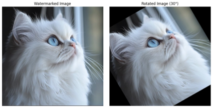
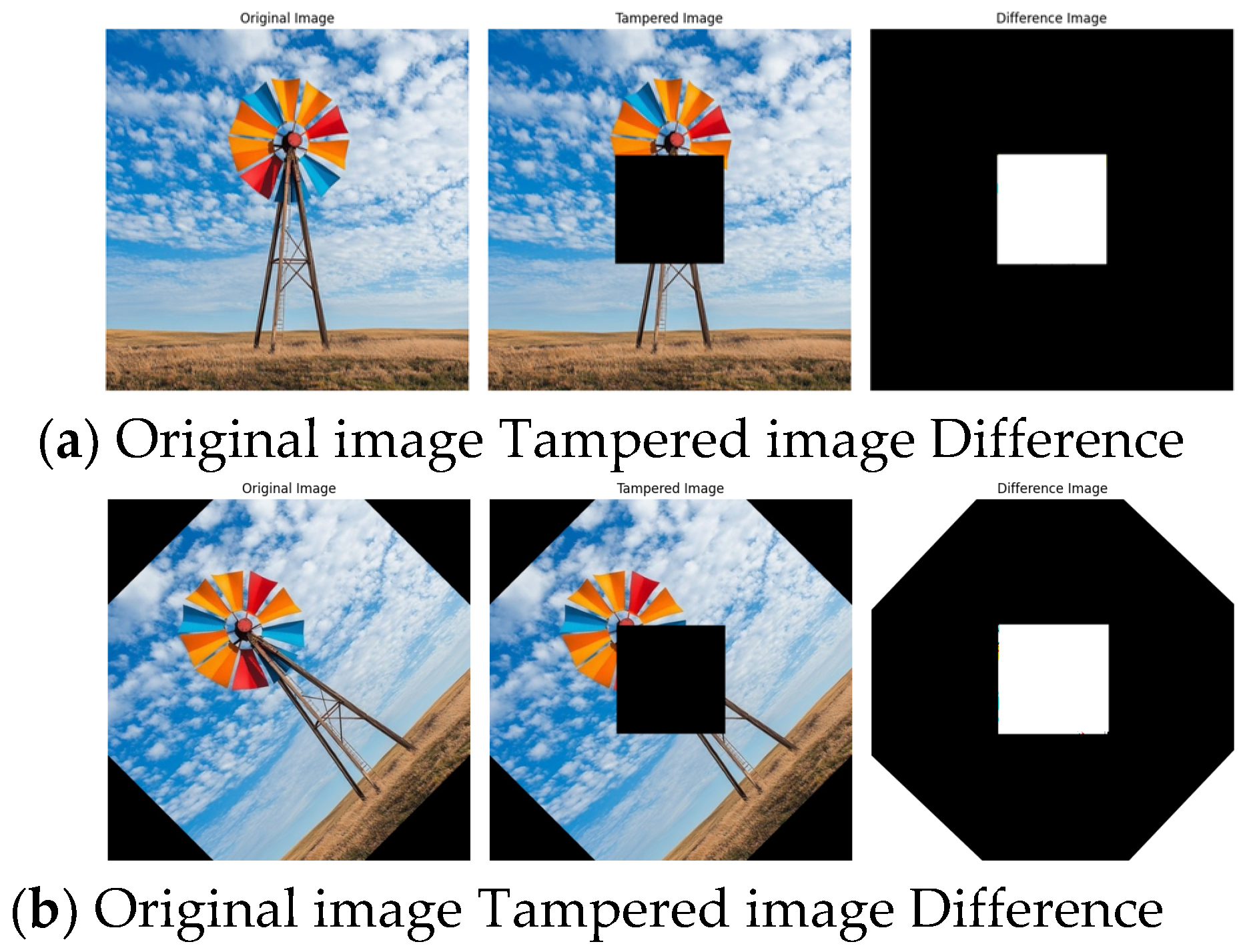
However, estimating $\theta$ is computationally expensive and often infeasible in blind or semi-blind scenarios, particularly when transformations are computed or non-rigid. Hence, the core problem lies in the geometric sensitivity and alignment dependency or traditional tamper detection mechanisms. This necessitates the development of transformation-invariant or geometrically robust detection frameworks capable of accurate tamper localization under arbitrary geometric distortions without prior knowledge of $T_{\theta }$. The pictorial illustration of image tampering in both the original and rotated image is shown in Figure 1a,b where a clear distinction is observed between the original image and the rotated image during tamper pixel detection, with a higher number of tampered pixels detected in the rotated image.

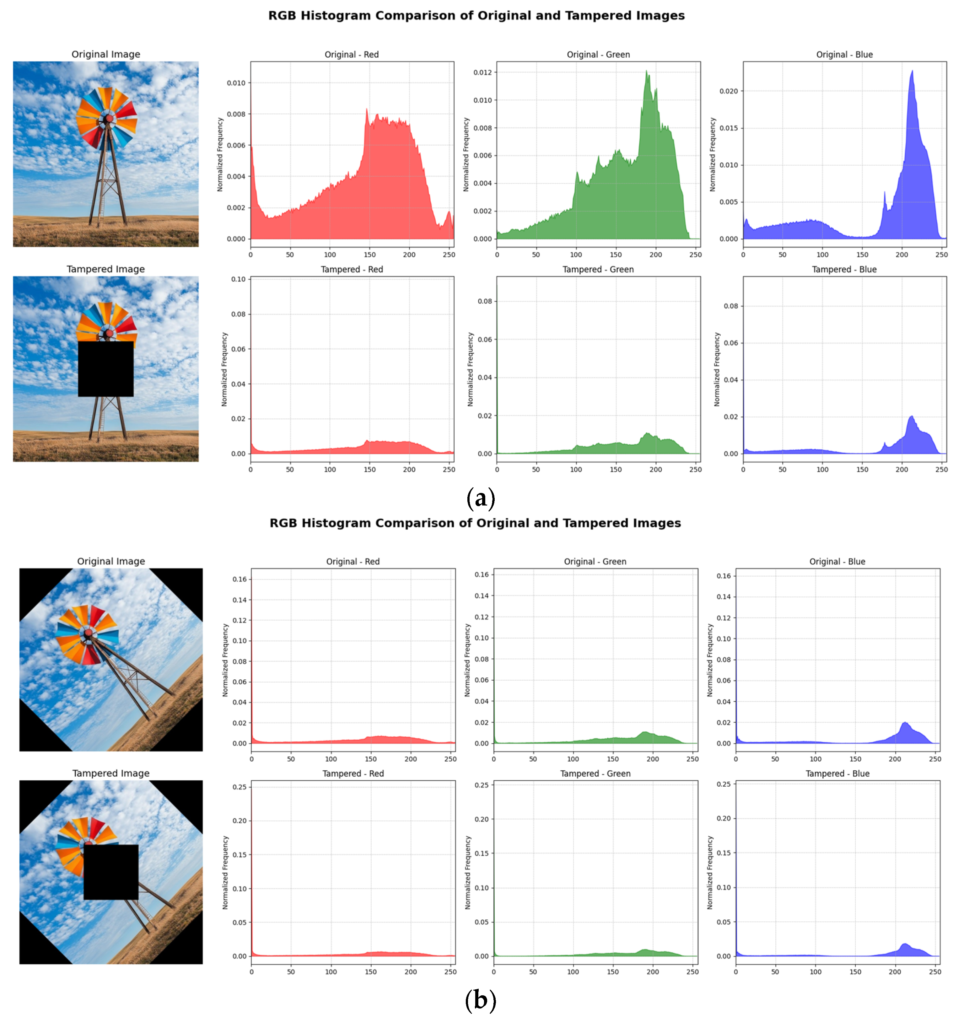
Additionally, the histogram analysis in Figure 2a,b highlights the differences between the original and geometrically transformed images.

The primary objective of this research is to develop a tamper detection framework that remains robust against TITO. Moreover, the major contributions of this work are listed as follows:

• A composite biometric watermark is created by merging a grayscale biometric image with the user’s personal signature, resulting in a fused watermark that strengthens identification association and boosts the distinctiveness of the embedded authentication data.
• The produced watermark fusion is integrated and subsequently retrieved via a hybrid transformation-domain watermarking system that employs the sequential application of DWT-DCT-SVD.
• Unlike traditional methods that rely on strict spatial alignment and pixel-wise comparison, the proposed approach leverages the rotation invariance of SIFT and ORB descriptors to detect tampering without prior knowledge of the transformation parameters. By establishing keypoint correspondences and validating them through homography estimation, the method enables accurate tamper localization under rotation. To quantify detection performance, several metrics such as average Euclidean distance, standard deviation of matched keypoints, number of strong matches, percentage of good matches, and homography residuals are employed.

The rest of the paper is assembled as follows: Section 2 reviews the relevant literature. Section 3 explains the proposed watermarking technique, including watermark fusion, hybrid embedding, extraction, watermark decoupling, and tamper detection with SIFT and ORB descriptors. Furthermore, Section 4 shows the experimental setup and result analysis with limitations. Finally, Section 5 provides concluding remarks and future directions.

2. Literature Review

Digital watermarking has emerged as a pivotal technique for intellectual property protection, content authentication, and secure communication in multimedia systems. Over the past decades, a substantial body of research has explored diverse methodologies to embed imperceptible yet robust watermarks into digital content, particularly images. Conventional watermarking approaches, leveraging spatial and transform domain techniques, have laid the foundational framework for reliable watermark embedding and extraction. However, the evolution of multimedia content, especially in the context of color imagery, has prompted advancements in perceptual modeling and chromatic data handling. Furthermore, the integration of local invariant descriptors, notably SIFT, has introduced a paradigm shift by enabling watermarking schemes that are highly resilient to geometric distortions and malicious attacks. In addition, hybrid embedding-based watermarking also offers significant embedding capacity (EC) and robustness. This section presents a comprehensive overview of these watermarking paradigms, delineating their corresponding techniques.

2.1. Grayscale-Oriented Image Encoding Techniques

Tang et al. [20] proposed a robust reversible watermarking (REW) technique that enhances embedding performance and image recovery through rounded error compensation. Yan et al. [21] presented a multi-watermarking scheme combining logo and text watermarks to ensure medical image integrity and confidentiality. Dai et al. [22] developed a hybrid watermarking model combining zero and REW for secure and verifiable medical image transmission. Gull et al. [23] introduced a self-embedding watermarking scheme based on the least significant bit (LSB) for tamper detection and localization. Ref. [24] proposed a block mapping mechanism leveraging singular value decomposition (SVD) and block truncation coding (BTC) wherein each block is associated with a reference block. The LSB embedding embeds recovery data of one block into its mapped counterpart, and vice versa. However, if a block is identified as tampered, its mapped block is also flagged, resulting in the “tamper coincidence problem” [25]. Tang et al. [26] enhanced the robustness of REW by employing polar harmonic transforms (PHTs) and attack simulations. Jana et al. [27] proposed a self-embedding FrW method using absolute moment block truncation code (AMBTC) applied to complex regions. Mao et al. [28] designed a content-aware quantization index modulation (QIM) algorithm that minimizes distortion using statistical data of cover images (CI). Lin et al. [29] extended AMBTC-based watermarking using vector quantization for recovery data and fragile authentication codes. Sahu [30] utilized a logistic map and XOR for blind FrW. A proficient encoding-based watermarking method for tamper detection and localization was presented in [31]. Hu et al. [32] proposed a robust watermarking that preserves gray image quality while withstanding geometric transformations. Bhalerao et al. [33] generated 16-bit watermarks via SHA-1 and XOR with block keys, embedded using LSB. Rijati et al. [34] integrated SHA-512-based authentication with layered embedding and feature super-resolution convolutional neural network (FSRCNN)-based recovery. He et al. [35] proposed enhancing REW fidelity through adaptive 2D mapping of prediction error pairs to minimize distortion during embedding. Ma et al. [36] introduced a symmetry-based watermarking technique using random patterns and autocorrelation to resist complex local geometric attacks. Zhang et al. [37] proposed a frequency domain watermarking scheme employing symmetric peaks for enhanced resilience against social media and geometric attacks. Fu et al. [38] leveraged fractional-order Zernike and pseudo-Zernike moments to achieve robust REW. Xiong et al. [39] developed a secure, robust REW scheme using lightweight cryptography and multi-party sharing. You et al. [40] improved the robustness with spread spectrum embedding using Hungarian optimization. Wang et al. [41] integrated UDCTWT and PHFMs with statistical modeling to enhance watermark imperceptibility and robustness.

2.2. Color-Oriented Image Encoding Techniques

Su et al. [42] proposed a robust and computationally efficient color image watermarking (CIW) scheme by fusing LU factorization with spatial domain processing, enabling real-time embedding and extraction without frequency transformation. Cheema et al. [43] introduced a semi-blind watermarking framework using FRT, DWT, and SVD for robust color image (CoI) protection. Al-Otum et al. [44] introduced a dual-domain CIW scheme (RFW-AT) that combines robust DWT-based and fragile LSB-based embedding for authentication and self-recovery. Sinhal et al. [45] proposed a blind FrW approach for tamper localization and recovery in RGB CoIs. Qiu et al. [46] presented a high-quality blind CIW scheme based on fast quaternion Schur decomposition. A client-side embedding watermarking scheme for screen-shooting resilience and watermark traceability on CoI was presented in [47]. Shi et al. [48] proposed a dual-watermarking scheme integrating block feature modulation scrambling (BFMS) and a voting mechanism with majority rule (VMMR) to achieve robust copyright protection and precise tampering detection in CoI. Zhang et al. [49] introduced a dual-defense framework incorporating adversarial and traceable watermarking for face swap attack mitigation in facial CoIs. Altaf et al. [50] proposed TDLCI, a FrW scheme for CoI tamper detection and localization, employing pixel differencing and a logistic map-based chaotic sequence for watermark embedding. Hao et al. [51] proposed a large-scale FrW scheme for images by leveraging prime number distribution theory and pixel parity encoding, enabling simultaneous embedding of multiple watermarks. Soualmi et al. [52] suggested a semi-fragile blind watermarking scheme for CoIs by integrating artificial bee colony optimization, BRISK features, and DCT, enabling robust embedding in perceptually significant regions. Chen et al. [53] presented a structure-preserving QSVD-based method for CIW, ensuring high fidelity and robustness through adaptive embedding and coefficient pair selection. Mehraj et al. [54] designed a DCT-based CIW scheme leveraging YCbCr space for cultural image protection. Hosny et al. [55] introduced a novel fractional-order exponent moment to enhance robustness in CIW.

2.3. SIFT-Oriented Image Encoding Techniques

Hamidi et al. [56] proposed a robust hybrid image watermarking scheme that integrated DWT-DCT and SIFT to achieve strong imperceptibility and resilience against both signal processing and geometric attacks. Fang et al. [57] proposed a robust zero-watermarking scheme for medical images by integrating SIFT-based preprocessing with bendlet-DCT feature extraction and tent map chaotic encryption, ensuring non-invasive and secure watermark embedding. Zhang et al. [58] presented an REW scheme for tamper detection and localization, leveraging SIFT-based feature extraction, histogram-based watermark generation, and dual embedding with RIWT and SVD for enhanced robustness. Gan et al. [59] introduced a robust screen-shooting resilient watermarking algorithm by integrating entropy-weighted Harris corner detection, SIFT-based feature region constriction, and adaptive-radius DFT embedding.

2.4. DWT-DCT-SVD-Oriented Image Encoding Techniques

Awasthi et al. [60] introduced two hybrid watermarking methodologies: DWT-DCT-SVD and lifting wavelet transform (LWT)-DCT-SVD. They enhanced embedding efficacy through JAYA optimization and particle swarm optimization (PSO) to ascertain a suitable scaling factor. Devi et al. [61] introduced a robust blind watermarking technique for medical images, specifically for computed tomography (CT), X-ray, magnetic resonance imaging (MRI), and ultrasound digital imaging and communications in medicine (DICOM) images, utilizing a gray wolf optimization (GWO)-DWT-DCT-SVD hybrid model. Arora et al. [62] proposed a safe hybrid watermarking technique for image authentication that integrates DWT, DCT, and SVD with Rivest–Shamir–Adleman (RSA) encryption and chaotic logistic map scrambling. Varghese et al. [63] introduced a hybrid digital watermarking methodology that integrates DWT, DFT, DCT, and SVD, embedding multiple watermark replicas within the frequency components of the host image.

3. Proposed Watermarking Scheme

This work proposes a hybrid watermarking scheme that leverages the two grayscale watermarks, such as a personal signature and a biometric fingerprint, into a color image. The individual watermarks are first preprocessed and fused to form a single composite watermark, enhancing both identity authentication and robustness. Then, both the embedding and extraction processes are performed in the transform domain by sequentially applying DWT-DCT-SVD. The following sections delineate the complete workflow of the proposed watermarking scheme, encompassing watermark fusion, embedding, extraction, watermark decoupling, and tamper detection.

3.1. Watermark Fusion

The fusion is performed at the bit-plane level, which makes it a spatial domain embedding to preserve perceptual transparency while embedding high-level identity features.

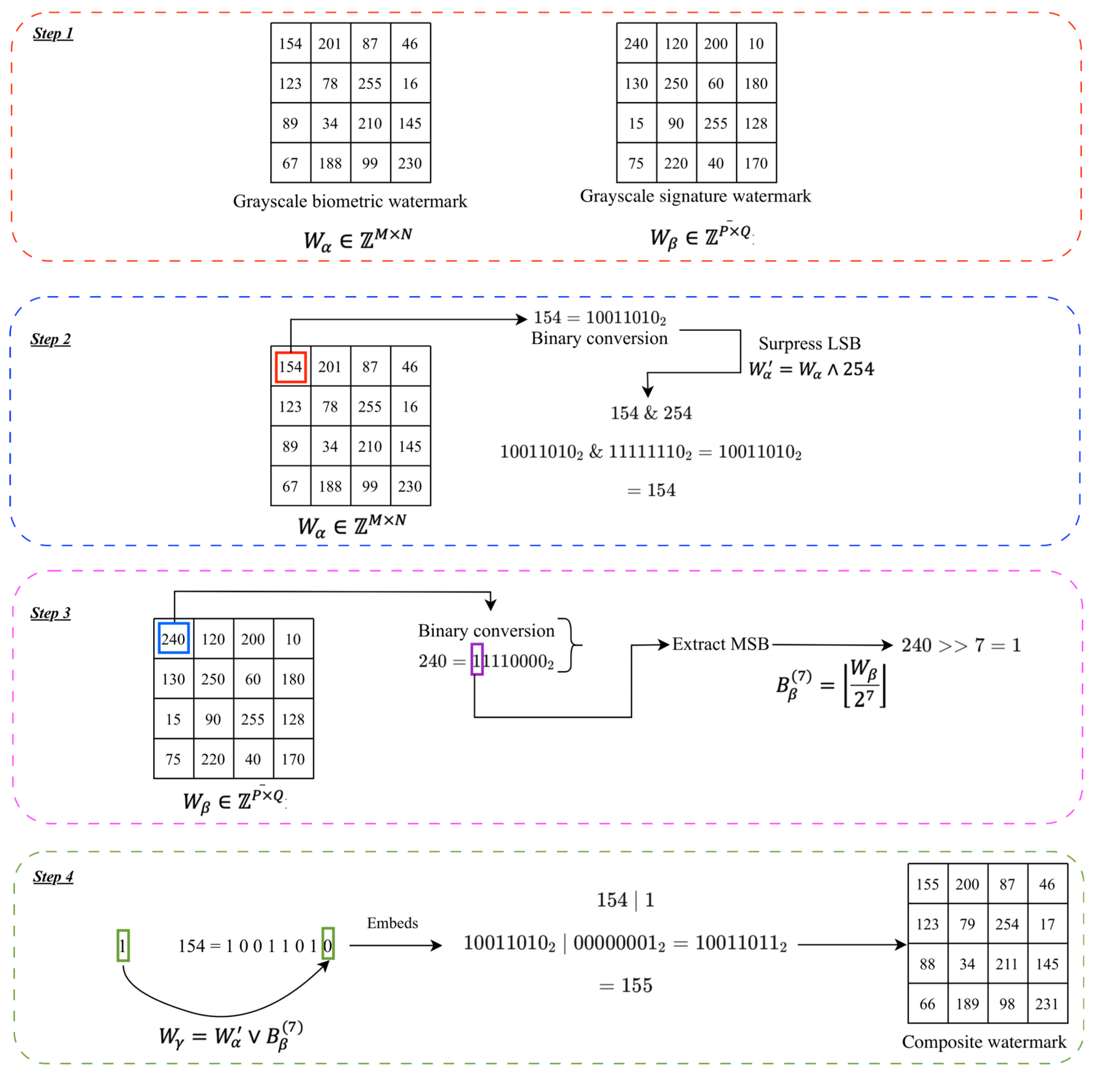
Step 1. Let $W_{\alpha }\in {\mathbb{Z}}^{M\times N}$ represent the grayscale biometric watermark (primary), and $W_{\beta }\in {\mathbb{Z}}^{P\times Q}$ represent the grayscale signature watermark (auxiliary).

Step 2. Suppress the LSB of each pixel in the biometric watermark:

$$W_{\alpha }^{\prime }=W_{\alpha }\wedge 254$$

(5)

Step 3. Isolate the most significant bits (MSBs) of each pixel in the signature watermark:

$$B_{\beta }^{(7)}=⌊{\displaystyle \frac{W_{\beta }}{2^7}}⌋$$

(6)

Step 4. Integrate the MSB of $W_{\beta }$ into the cleared LSB of $W_{\alpha }$ to generate the composite watermark:

$$W_{\gamma }=W_{\alpha }^{\prime }\vee B_{\beta }^{\left(7\right)}$$

(7)

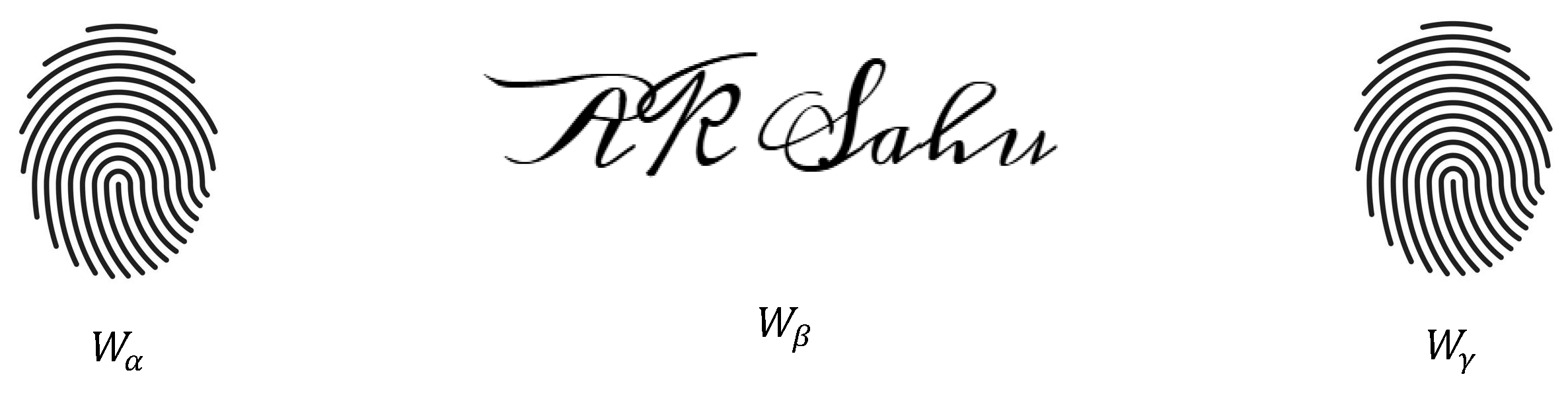
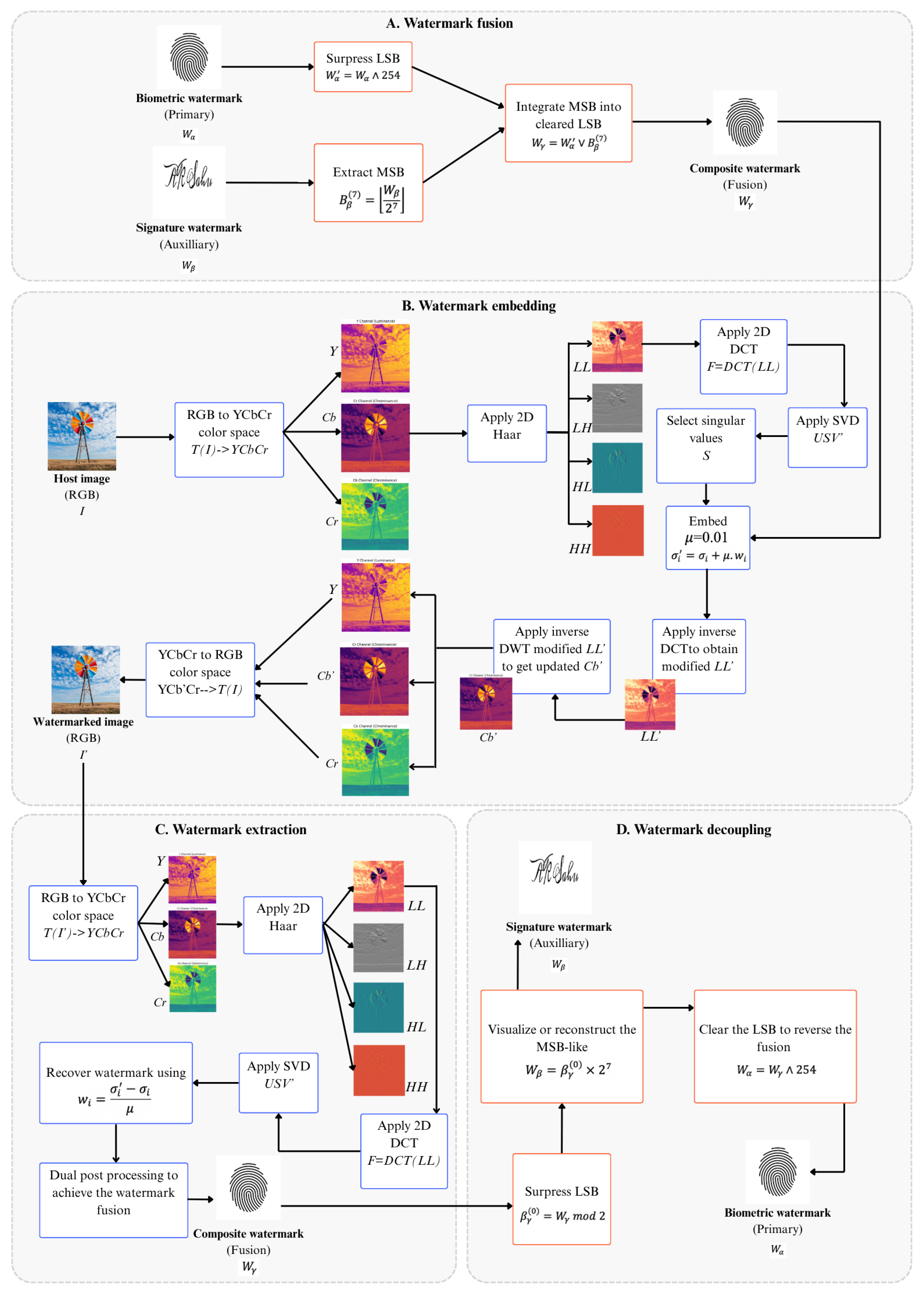
$W_{\gamma }$ is a perceptually indistinguishable image depicted in Figure 3 from $W_{\alpha }$, yet semantically enriched with high-order features from $W_{\beta }$. Furthermore, the entire process is depicted in Figure 4 using a numerical example for the reader’s convenience. Additionally, Algorithm 1 represents the pseudocode of the watermark fusion.

Algorithm 1. Watermark Fusion

1:   Input: C, H    ▷ Biometric and signature grayscale images, same size 2:   Output: E      ▷ Fused watermark 3:   procedure LSB-EMBED (C, H, E) 4:               resize H to size of C 5:               c ← array(C), h ← array(H) 6:               for each pixel p in c do 7:                          c′ ← c [p] AND 0xFE      ▷ clear LSB of biometric pixel 8:                          b ← h [p] >> 7                 ▷ extract MSB of signature pixel 9:                          E [p] ← c′ OR b               ▷ embed hidden MSB into biometric LSB 10:               end for 11:               save E as image file                   ▷ cast to uint8 before saving 12:               display c, h, E side by side 13:               print “Embedded watermarks displayed successfully.” 14:   end procedure

3.2. Watermark Embedding

The procedure for cascaded transform domain embedding is outlined in the following steps. In addition, Algorithm 2 represents the pseudocode of the watermark embedding.

Step 1. Let the host image $I_{RGB}\in {\mathbb{R}}^{M\times N\times 3}$ be transformed into the YCbCr color space to isolate the luminance and chrominance components:

$$I_{YCbCr}=RGB2YCbCr\left(I_{RGB}\right)$$

(8)

Subsequently, the individual channels Y, Cr, and Cb are extracted.

Step 2. A single-level 2D DWT is applied to the Cb channel using the Haar wavelet, resulting in the decomposition

$$C_b\stackrel{ DWT }{\to }\{C_b^{LL},C_b^{LH},C_b^{HL},C_b^{HH}\}$$

(9)

Step 3. The low-frequency approximation subband $C_b^{LL}$ is further transformed via the 2D DCT to exploit its energy compaction property:

$$D=DCT\left(C_b^{LL}\right)$$

(10)

This transformation concentrates the significant image information into a smaller set of low-frequency coefficients.

Step 4. The resulting DCT matrix $D$ is factorized using SVD to produce three matrices, i.e., $U\in {\mathbb{R}}^{m\times m}, V\in {\mathbb{R}}^{n\times n}$ (orthogonal matrices) and $\Sigma \in {\mathbb{R}}^{m\times n}$ (diagonal matrix), containing the singular values ${\sigma }_i$. Afterwards, extract the vector of singular values $\overrightarrow{\sigma }={\left[{\sigma }_1,{\sigma }_2,\dots .,{\sigma }_r\right]}^T, r=min(m,n)$.

Step 5. The combined watermark $W_{\gamma }\in {\mathbb{R}}^{k\times k}$ is resized in such a way that $k=⌊\surd r⌋$. Flatten and normalize the watermark:

$$\overrightarrow{w}={\displaystyle \frac{vec\left(W_{\gamma }\right)}{255}}, \overrightarrow{w}\in {\left[0,1\right]}^{k^2}$$

(11)

Step 6. Embed the watermark into the singular values using an embedding strength factor $\mu$:

$${\sigma }_i^{\prime }={\sigma }_i+\mu .w_i, \mathrm{for} i=1, 2,\dots ., k^2$$

(12)

The proposed scheme has taken $\mu$ = 0.01, 0.02, 0.03, and 0.04 to differentiate the imperceptibility and robustness. Now, construct the modified diagonal matrix ${\Sigma }^{\prime }=diag({\overrightarrow{\sigma }}^{\prime })$.

Step 7. Using the modified singular values, reconstruct the modified DCT coefficient matrix $D^{\prime }=U.{\Sigma }^{\prime }.V^T$. Then, apply inverse DCT to obtain the modified LL subband $C_b^{{LL}^{\prime }}$.

Step 8. Reconstruct the modified Cb channel using the original detail subbands and the modified approximation subband by performing inverse DWT:

$$C_b^{\prime }\stackrel{ IDWT }{\to }\left\{C_b^{{LL}^{\prime }},C_b^{LH},C_b^{HL},C_b^{HH}\right\}$$

(13)

Clip values to maintain a valid pixel range as $C_b^{\prime }=clip(C_b^{\prime },0,255)$. Now, convert that into an 8-bit image represented by $C_b^{\prime }=C_b^{\prime }.astype(uint8)$.

Step 9. Reconstruct the modified YCbCr image:

$$I_{YCbCr}^{\prime }=merge\left(Y, Cr, C_b^{\prime }\right)$$

(14)

Finally, convert $I_{YCbCr}^{\prime }$ back to RGB:

$$I_{RGB}^{\prime }=YCbCr2RGB\left(I_{YCbCr}^{\prime }\right)$$

(15)

The resulting image $I_{RGB}^{\prime }$ is the final watermarked image.

Algorithm 2. DWT-DCT-SVD Watermark Embedding
1: Input: H (host image, RGB), W (watermark, grayscale), α (embedding strength)
2: Output: H’ (watermarked image, RGB)
3:	procedure Embed Watermark (H, W, α)
4:	Convert Hp5G → Y, Cr, Cb                                           ▷ RGB to YCrCb color space
5:	LL, (LH, HL, HH) ← DWT (Cb, Haar)                       ▷ 1-level Haar DWT on Cb
6:	D ← DCT(LL)                                                                ▷ Apply 2D DCT on LL subband
7:	U, S, V ← SVD(D)                                                          ▷ Singular value decomposition
8:	s ← ⌊√|S|⌋                                                   ▷ Watermark side length from # singular values
9:	Resize W to s × s; normalize:   W’← W / 255
10:	S’ ← copy of S
11:	for i → 0, s−1   do
12:	for j → 0, s−1   do
13:	k ← i·s + j                                        ▷ Flat index into S
14:	if k < |S|   then
15:	S’[k] ← S[k] + α · W’[i, j]            ▷ Embed watermark pixel
16:	end if
17:	end for
18:	end for
19:	D’ ← U · diag(S’) · V                                     ▷ Reconstruct modified DCT matrix
20:	LL’ ← IDCT(D’)                                             ▷ Inverse DCT
21:	Cb’ ← IDWT ((LL’, (LH, HL, HH)), Haar)         ▷ Inverse DWT
22:	Clip Cb’ to [0, 255] and cast to uint8
23:	Merge Y, Cr, Cb’ → H’pycRcb
24:	Convert H’pycRcb → H’pGB
25:	return H’pGB
26:	end procedure

3.3. Watermark Extraction

The watermark extraction procedure is systematically described in the succeeding steps. Furthermore, Algorithm 3 represents the pseudocode of the watermark extraction.

Step 1. Convert the watermarked RGB image $I_{RGB}^{\prime }\in {\mathbb{R}}^{M\times N\times 3}$ into YCbCr color space. Then, decompose the image into its luminance and chrominance components $Y_{wm},C_r^{wm}, C_b^{wm}$.

Step 2. Apply a single-level 2D Haar DWT to the watermarked Cb channel:

$$C_b^{wm}\stackrel{ DWT }{\to }\left\{C_b^{{LL}^{\prime }},C_b^{LH},C_b^{HL},C_b^{HH}\right\}$$

(16)

The approximation subband $C_b^{{LL}^{\prime }}$ contains the watermark-influenced signal components.

Step 3. Perform the 2D DCT on $C_b^{{LL}^{\prime }}$ to transition into the frequency domain. Additionally, this aligns the domains with the one used during embedding.

Step 4. Decompose the DCT matrix using SVD:

$$D^{\prime }=U_{wm}.{\Sigma }^{\prime }.V_{wm}^T$$

(17)

Extract the singular values, i.e., ${\overrightarrow{\sigma }}^{\prime }=diag\left({\Sigma }^{\prime }\right)={\left[{\sigma }_1^{\prime },{\sigma }_2^{\prime },\dots ,{\sigma }_r^{\prime }\right]}^T$.

Step 5. Since the original singular values $\overrightarrow{\sigma }$ are known, the watermark is accurately recovered using

$$w_i={\displaystyle \frac{{\sigma }_i^{\prime }-{\sigma }_i}{\mu }}, \forall i=1,2,..,k^2$$

(18)

Note that $\mu$ = 0.01, 0.02, 0.03, and 0.04 during extraction.

Reshape the recovered watermark vector $W_{{\gamma }_{ext}}$ into the 2D matrix using $reshape(\overrightarrow{w},\left[k,k\right])$. Where $k=⌊\surd r⌋$, assuming a square watermark.

Step 6. This step offers two alternative post-processing paths, normalizing or binarizing the extracted watermark based on the requirement. Normalization employs the $W_{{\gamma }_{rec}}=clip(255.W_{{\gamma }_{ext}},0,255)$ function, whereas binarization utilizes the $W_{{\gamma }_{bin}}(i,j)=\left\{\begin{array}{c}1, if W_{{\gamma }_{ext}}\left(i,j\right)>T\\ 0, otherwise\end{array} ,T\in [0,1]\right.$ condition where T is the threshold. Therefore, the final matrix $W_{{\gamma }_{rec}}$ or $W_{{\gamma }_{bin}}$ represents the extracted watermark fusion. Figure 5 depicts the complete architecture of the embedding and extraction procedure.

Algorithm 3. DWT-DCT-SVD Watermark Extraction
1: Input: Iw (watermarked RGB image), α (embedding strength)
2: Output: Wb (extracted binary watermark)
3:	Procedure Extract Watermark (Iw, α)
4:	Convert Iw → Y, Cr, Cb                                            ▷ RGB to YCrCb color space
5:	LL, (LH, HL, HH) ← DWT (Cb, Haar)                  ▷ 1-level Haar DWT on Cb
6:	D ← DCT(LL)                                                           ▷ Apply 2D DCT on LL subband
7:	U, S, V ← SVD(D)                                                     ▷ Singular value decomposition
8:	m ← ⌊√|S|⌋                                                              ▷ Side length of extracted watermark
9:	Initialize W ← zero matrix of size m × m
10:	for i ← 0 to m − 1 do
11:	for j ← 0 to m − 1 do
12:	k ← i · m + j                                               ▷ Flat index into S
13:	if k < |S| then
14:	W [i, j] ← (S[k] − min(S)) / α              ▷ Recover watermark value
15:	end if
16:	end for
17:	end for
18:	Normalize W into range [0, 1]
19:	Wb ← (W > 0.5) × 255                                              ▷ Convert into binary watermark
20:	return Wb
21:	end procedure

3.4. Watermark Decoupling

The objective is to extract high-order identity features of the auxiliary gray watermark from the composite biometric watermark image. Algorithm 4 represents pseudocode of the watermark decoupling.

Step 1. Define the grayscale composite watermark image $W_{\gamma }\in {\mathbb{Z}}^{M\times N}$ extracted from section C, where each pixel value lies in the integer domain [0, 255], i.e., $W_{\gamma }\left(i,j\right)\in \{0,1,\dots ,255\}$.

Step 2. Retrieve the LSB plane from the composite watermark by applying a modulo-2 operation element-wise:

$${\beta }_{\gamma }^{(0)}=W_{\gamma } mod 2$$

(19)

Here, ${\beta }_{\gamma }^{(0)}\in {\{0,1\}}^{M\times N}$ represents the binary matrix capturing the LSB layer of $W_{\gamma }$.

Step 3. To visualize or reconstruct the MSB-like version of the auxiliary watermark,

$$W_{\beta }={\beta }_{\gamma }^{(0)}\ll 7={\beta }_{\gamma }^{(0)}\times 2^7$$

(20)

This operation transforms binary elements {0,1} into {0,128}, effectively creating a pseudo-MSB image $W_{\beta }\in {\{0,128\}}^{M\times N}$ for visualization or high-order approximation purposes.

Step 4. Clear the LSB of each pixel in the composite image by applying a bitwise AND operation with mask 254 to reverse the fusion:

$$W_{\alpha }=W_{\gamma }\wedge 254=W_{\gamma }\wedge (2^8-2)$$

(21)

Algorithm 4. Watermark Decoupling
1:	Input: E                                                       ▷ fused grayscale watermark image
2:	Output: H, C                                             ▷ extracted signature and recovered biometric image
3:	procedure LSB-EXTRACT (E, H, C)
4:	e ← array(E)
5:	for each pixel p in e do
6:	b ← e[p] AND 0x01                             ▷ extract hidden bit from LSB
7:	H[p] ← b × 255                                     ▷ expand bit to visible grayscale
8:	C[p] ← e[p] AND 0xFE                     ▷ clear LSB to recover cover watermark
9:	end for
10:	display E, H, C side by side
11:	end procedure

3.5. Tamper Detection Using SIFT and ORB

Tamper detection is a critical component in digital watermarking, ensuring the integrity and authenticity of the content by identifying unauthorized alterations. This work employs SIFT and ORB to effectively detect tampering by extracting and matching distinctive keypoint between the original and potentially altered images. SIFT identifies keypoints by locating extrema in the Difference of Gaussian (DoG) scale space, mathematically represented as

$$D\left(x,y,\sigma \right)=\left(G\left(x,y,k\sigma \right)-G\left(x,y,\sigma \right)\right)\ast I\left(x,y\right)$$

(22)

where G is the Gaussian function, I is the input image, and k is a constant multiplicative factor controlling scale.

Meanwhile, ORB combines the FAST keypoint detector with the BRIEF descriptor, enhanced by orientation compensation to maintain invariance:

$$ORB\left(p\right)=BRIEF\left(rotate\left(p,\theta \right)\right)$$

(23)

Here, p denotes the keypoint location and $\theta$ is the keypoint orientation.

The following steps elaborate on the tamper detection procedure. Afterwards, Algorithm 5 represents pseudocode of the tamper detection.

Step 1. Load $I_{RGB}\in {\mathbb{R}}^{M\times N\times 3}$ and ${I^{\prime }}_{RGB}\in {\mathbb{R}}^{M\times N\times 3}$ in grayscale as $I_O\in {\mathbb{R}}^{m\times n}$ and $I_w\in {\mathbb{R}}^{m\times n}$ respectively to standardize intensity levels, ensuring $I_O,I_w:\mathrm{\Omega }⟶\mathbb{R}$, where $\mathrm{\Omega }$ denotes the image domain.

Step 2. Construct the scale-space representation $D\left(x,y,\sigma \right)$ from Equation (22) by convolving $I$ with Gaussian Kernels $G\left(x,y,k\sigma \right)$.

Step 3. Compute the DoG function from Equation (22) to identify scale-space extrema.

Step 4. Detect keypoints $\left\{k_i^{SIFT}\right\}$ by localizing extrema in $D\left(x,y,\sigma \right)$ across scales.

Step 5. For each $k_i^{SIFT}$, compute a descriptor vector $d_i^{SIFT}\in {\mathbb{R}}^{128}$ encoding gradient orientations in the neighborhood.

Step 6. Detect keypoints $\left\{k_j^{ORB}\right\}$ using the FAST corner detector algorithm with orientation compensation which uses $k_j^{ORB}=FAST\left(I,threshold\right), {\theta }_j=orientation\left(k_j^{ORB}\right)$ functions.

Step 7. Compute binary descriptors $d_j^{ORB}\in {\{0,1\}}^n$ using the rotated BRIEF method to maintain rotation invariance:

$$d_j^{ORB}=BRIEF\left(RotatedPatch\left(I,k_j^{ORB},{\theta }_j\right)\right)$$

(24)

Step 8. For SIFT, initialize a brute-force matcher using Euclidean distance metric ${BF}_{SIFT}=BFMatcher(d,norm={\left|\right|.\left|\right|}_2)$.

Step 9. For ORB, initialize a brute-force matcher using Hamming distance suitable for binary descriptors ${BF}_{ORB}=BFMatcher(d,norm=Hamming)$.

Step 10. Now compute pairwise matches between the $I_O$ and $I_w$ descriptors $d_i^{SIFT}$ and $k_j^{ORB}$. The matcher returns matches $M_{SIFT}$ and $M_{ORB}$, where each match associates a descriptor from $I_O$ to the closest descriptor in $I_w$.

Step 11. Sort the valid matches $M_{sorted}$ based on their matching distance $d(m)$, where a lower indicates a better match.

Step 12. Create a binary mask $T\in {\left\{0,1\right\}}^{m\times n}$ initialized to zero. For each match $m_l\in M_{sorted}$, examine the matching distance $d(m_l)$.

Step 13. If $d(m_l)>\mathcal{T}$, then mark the corresponding keypoint location in $I_w$ as tampered. Then extract the keypoint position in the $I_w$. Here, $\mathcal{T}$ is the threshold or tampering rate that differs for SIFT and ORB due to their descriptor scales. The $\mathcal{T}$ values are taken as, 5%, 30%, 60%, 90%, and 100% for SIFT and 5%, 10%, 20%, 30%, and 50% for ORB respectively.

Algorithm 5. SIFT–ORB-based Tamper Detection
1:	Input: Io, It                                                                    ▷ Original and test images
2:	Output: Ms, Mo                                                  ▷ SIFT- and ORB-based tamper masks
3:	procedure DETECT (Io, It, Ms, Mo)
4:	read Io, It in grayscale                                                      ▷ input images
5:	(K1, D1) ← SIFT(Io)                                                         ▷ SIFT on original image
6:	(K2, D2) ← SIFT(It)                                                         ▷ SIFT on test image
7:	Ls ← BF_L2(D1, D2)                                                       ▷ brute-force matching
8:	sort Ls by d(m)                                                                    ▷ ascending distance
9:	Ms ← 0                                                                                 ▷ initialize SIFT mask
10:	for each m ∈ Ls do
11:	if d(m) > Ts then                                                           ▷ mismatched pair
12:	p ← K2[mt]                                                            ▷ location in test image
13:	Ms(p) ← 1                                                              ▷ mark tampered point
14:	end if
15:	end for
16:	(K3, D3) ← ORB (Io)                                                            ▷ ORB on original image
17:	(K4, D4) ← ORB (It)                                                              ▷ ORB on test image
18:	Lo ← BF_H (D3, D4)                                               ▷ brute-force Hamming matching
19:	sort Lo by d(m)                                                              ▷ ascending distance
20:	Mo ← 0                                                                                 ▷ initialize ORB mask
21:	for each m ∈ Lo do
22:	if d(m) > To then                                                        ▷ mismatched pair
23:	q ← K4 [mt]                                                         ▷ location in test image
24:	Mo(q) ← 1                                                           ▷ mark tampered point
25:	end if
26:	end for
27:	return Ms, Mo                                                                    ▷ output masks
28:	end procedure

4. Experimental Setup and Result Analysis

A set of 24 standard 24-bit color images with a resolution of $512\times 512$ pixels was used in extensive experiments to assess the efficacy of the proposed watermarking scheme. In addition, the proposed scheme was tested against the CASIA 1.0 public forged dataset to demonstrate the tamper localization efficiency. All experiments were conducted using a MacBook Air equipped with the Apple M1 chip, 8 GB RAM, and 256 GB SSD storage, while the implementation and simulation environment were realized in Google Colab using a Python 3.12.13 version. A grayscale fingerprint and biometric watermarks, each measuring $512\times 512$ pixels, were embedded as watermark data in each cover image. The following commonly used objective metrics were employed to rigorously quantify the watermarking scheme’s robustness and imperceptibility: mean squared error (MSE), peak signal-to-noise ratio (PSNR), structural similarity index measure (SSIM), normalized cross-correlation (NCC), bit error rate (BER), true positive (TP), true negative (TN), false positive (FP), false negative (FN), accuracy, precision, Matthews correlation coefficient (MCC), recall, F1-score, receiver operating characteristic (ROC) point, and intersection over union (IoU).

Table 1. Image dataset (cover images and watermarks).

Cover Images
$I_{RGB}^1$	$I_{RGB}^2$	$I_{RGB}^3$	$I_{RGB}^4$	$I_{RGB}^5$	$I_{RGB}^6$
$I_{RGB}^7$	$I_{RGB}^8$	$I_{RGB}^9$	$I_{RGB}^{10}$	$I_{RGB}^{11}$	$I_{RGB}^{12}$
$I_{RGB}^{13}$	$I_{RGB}^{14}$	$I_{RGB}^{15}$	$I_{RGB}^{16}$	$I_{RGB}^{17}$	$I_{RGB}^{18}$
$I_{RGB}^{19}$	$I_{RGB}^{20}$	$I_{RGB}^{21}$	$I_{RGB}^{22}$	$I_{RGB}^{23}$	$I_{RGB}^{24}$
Watermarks
Biometric	Signatures $W_{\beta }$($W_{\beta 1}, W_{\beta 2}, W_{\beta 3}$)
$W_{\alpha }$	$W_{\beta 1}$		$W_{\beta 2}$	$W_{\beta 3}$

presents the cover images accompanied by the watermarks.

$$MSE={\displaystyle \frac{1}{M\times N}}{\sum }_{x=1}^M{\sum }_{y=1}^N{\left[CI\left(x,y\right)-WI\left(x,y\right)\right]}^2$$

(25)

$$PSNR=10{log}_{10}\left({\displaystyle \frac{{255}^2}{MSE}}\right)$$

(26)

$$SSIM\left(x , y\right)={\displaystyle \frac{\left(2{\mu }_x{\mu }_y+C_1\right)\left(2{\sigma }_{xy}+C_2\right)}{\left({\mu }_x^2+{\mu }_y^2+C_1\right)\left({\sigma }_x^2+{\sigma }_y^2+C_2\right)}}$$

(27)

$$NCC={\displaystyle \frac{{\sum }_{i=1}^M{\sum }_{j=1}^N\left(CI\left(i,j\right)-\overline{CI}\right)\left(WI\left(i,j\right)-\overline{WI}\right)}{\sqrt{{\sum }_{i=1}^M{\sum }_{j=1}^N{\left(CI\left(i,j\right)-\overline{CI}\right)}^2.{\sum }_{i=1}^M{\sum }_{j=1}^N{\left(WI\left(i,j\right)-\overline{WI}\right)}^2}}}$$

(28)

$$BER={\displaystyle \frac{Number of erroneous bits}{Total number of watermarked bits}}$$

(29)

$$Accuracy={\displaystyle \frac{TP+TN}{TP+TN+FP+FN}}$$

(30)

$$Precision={\displaystyle \frac{TP}{TP+FP}}$$

(31)

$$MCC={\displaystyle \frac{\left(TP\times FN\right)-\left(FP\times FN\right)}{\sqrt{\left(TP+FP\right)\left(TP+FN\right)\left(TN+FP\right)(TN+FN)}}}$$

(32)

$$Recall={\displaystyle \frac{TP}{TP+FN}}$$

(33)

$$F1score=2.{\displaystyle \frac{Precision . Recall}{Precision+Recall}}$$

(34)

$$ROC=\left\{\left(FPR\left(T\right),TPR\left(T\right)\right)|T\in [0,1]\right\}$$

(35)

$$IoU={\displaystyle \frac{Area of Overlap }{Area of Union}}$$

(36)

Here, area of overlap is the common area between the detected region and the true tampered region, whereas area of union is the total area covered by both regions together.

Furthermore,

Table 2. PSNR, SSIM, MSE, NCC, and BER values for $\mu =0.01$.

Images	PSNR (dB)	SSIM	MSE	NCC	BER
$I_{RGB}^1$	55.34 $\pm$$0.03$	0.9999 $\pm$$0.11$	0.1324 $\pm$$0.04$	0.9781 $\pm$$0.11$	0.0001 $\pm$$0.03$
$I_{RGB}^2$	55.23 $\pm$$0.23$	0.9895 $\pm$$0.04$	0.2314 $\pm$$0.03$	0.9882 $\pm$$0.22$	0.0231 $\pm$$0.10$
$I_{RGB}^3$	55.23 $\pm$$0.14$	0.9898 $\pm$$0.21$	0.2331 $\pm$$0.21$	0.9792 $\pm$$0.03$	0.0131 $\pm$$0.06$
$I_{RGB}^4$	55.13 $\pm$$0.04$	0.9992 $\pm$$0.05$	0.1342 $\pm$$0.21$	0.9795 $\pm$$0.12$	0.0432 $\pm$$0.11$
$I_{RGB}^5$	55.10 $\pm$$0.06$	0.9995 $\pm$$0.06$	0.1650 $\pm$$0.10$	0.9898 $\pm$$0.06$	0.0233 $\pm$$0.13$
$I_{RGB}^6$	55.29 $\pm$$0.05$	0.9998 $\pm$$0.13$	0.3412 $\pm$$0.06$	0.9891 $\pm$$0.05$	0.0234 $\pm$$0.21$
$I_{RGB}^7$	55.19 $\pm$$0.10$	0.9988 $\pm$$0.03$	0.2413 $\pm$$0.11$	0.9895 $\pm$$0.13$	0.0275 $\pm$$0.06$
$I_{RGB}^8$	55.21 $\pm$$0.11$	0.9990 $\pm$$0.14$	0.2202 $\pm$$0.21$	0.9802 $\pm$$0.20$	0.0178 $\pm$$0.03$
$I_{RGB}^9$	55.25 $\pm$$0.02$	0.9991 $\pm$$0.12$	0.2312 $\pm$$0.04$	0.9792 $\pm$$0.07$	0.0321 $\pm$$0.09$
$I_{RGB}^{10}$	55.23 $\pm$$0.13$	0.9987 $\pm$$0.03$	0.2245 $\pm$$0.03$	0.9795 $\pm$$0.03$	0.0319 $\pm$$0.06$
$I_{RGB}^{11}$	55.20 $\pm$$0.07$	0.9990 $\pm$$0.10$	0.1980 $\pm$$0.21$	0.9882 $\pm$$0.09$	0.0325 $\pm$$0.11$
$I_{RGB}^{12}$	55.15 $\pm$$0.05$	0.9899 $\pm$$0.05$	0.1879 $\pm$$0.08$	0.9898 $\pm$$0.06$	0.0222 $\pm$$0.09$
$I_{RGB}^{13}$	55.16 $\pm$$0.04$	0.9993 $\pm$$0.08$	0.1945 $\pm$$0.11$	0.9901 $\pm$$0.07$	0.0023 $\pm$$0.21$
$I_{RGB}^{14}$	55.31 $\pm$$0.13$	0.9996 $\pm$$0.06$	0.2140 $\pm$$0.21$	0.9794 $\pm$$0.21$	0.0311 $\pm$$0.13$
$I_{RGB}^{15}$	55.30 $\pm$$0.07$	0.9994 $\pm$$0.03$	0.1342 $\pm$$0.10$	0.9797 $\pm$$0.03$	0.0241 $\pm$$0.10$
$I_{RGB}^{16}$	55.27 $\pm$$0.09$	0.9997 $\pm$$0.05$	0.1728 $\pm$$0.09$	0.9880 $\pm$$0.16$	0.0245 $\pm$$0.03$
$I_{RGB}^{17}$	55.19 $\pm$$0.02$	0.9987 $\pm$$0.12$	0.1531 $\pm$$0.20$	0.9883 $\pm$$0.09$	0.0320 $\pm$$0.13$
$I_{RGB}^{18}$	55.21 $\pm$$0.13$	0.9991 $\pm$$0.05$	0.2446 $\pm$$0.05$	0.9889 $\pm$$0.10$	0.0224 $\pm$$0.09$
$I_{RGB}^{19}$	55.15 $\pm$$0.10$	0.9989 $\pm$$0.13$	0.1332 $\pm$$0.20$	0.9887 $\pm$$0.13$	0.0435 $\pm$$0.07$
$I_{RGB}^{20}$	55.27 $\pm$$0.02$	0.9990 $\pm$$0.07$	0.2564 $\pm$$0.11$	0.9888 $\pm$$0.06$	0.0227 $\pm$$0.21$
$I_{RGB}^{21}$	55.30 $\pm$$0.15$	0.9991 $\pm$$0.06$	0.1824 $\pm$$0.21$	0.9882 $\pm$$0.14$	0.0433 $\pm$$0.11$
$I_{RGB}^{22}$	55.26 $\pm$$0.05$	0.9992 $\pm$$0.13$	0.2232 $\pm$$0.05$	0.9878 $\pm$$0.11$	0.0327 $\pm$$0.03$
$I_{RGB}^{23}$	55.28 $\pm$$0.13$	0.9994 $\pm$$0.08$	0.1533 $\pm$$0.11$	0.9880 $\pm$$0.05$	0.0429 $\pm$$0.12$
$I_{RGB}^{24}$	55.31 $\pm$$0.02$	0.9993 $\pm 0.12$	0.2143 $\pm$$0.20$	0.9879 $\pm$$0.16$	0.0246 $\pm$$0.13$

reports the PSNR, SSIM, MSE, NCC and BER for $\mu =0.01$ between the $I_{RGB}$ and ${I^{\prime }}_{RGB}$. For robustness analysis, each experiment was repeated three independent times with three different watermarks. The values reported in the table for PSNR, SSIM, MSE, NCC, and MER are expressed as mean ± standard deviation over these three runs. The deviation indicates values below 0.25, demonstrating resilience.

The highest PSNR value of 55.34 dB is observed for $I_{RGB}^1$, indicating minimal distortion, while the lowest PSNR value of 55.10 dB occurs for $I_{\mathit{RGB}}^5$. The SSIM values range from a minimum of 0.9895 ($I_{RGB}^2$) to a maximum of 0.9999 ($I_{RGB}^1$ and $I_{RGB}^6$), reflecting high structural similarity across all images. In terms of MSE, $I_{RGB}^6$ exhibits the highest error at 0.3412, whereas the lowest MSE of 0.1324 is recorded for $I_{RGB}^1$, further confirming the fidelity of the reconstruction. Afterwards, the calculation of NCC reveals that the highest value is 0.9901 for $I_{RGB}^{13}$. Similarly, the lowest NCC of 0.9781 is obtained by $I_{RGB}^1$. Finally, $I_{RGB}^1$ achieves the lowest BER of 0.0001, which indicates perfect extraction and no bit error, whereas $I_{RGB}^1$ obtains the highest BER of 0.0432, which also indicates the robustness of the watermark.

Table 3. PSNR, SSIM, MSE, NCC, and BER values for $\mu =0.02$.

Images	PSNR (dB)	SSIM	MSE	NCC	BER
$I_{RGB}^1$	53.25 $\pm$$0.04$	0.9898 $\pm$$0.06$	0.2314 $\pm$$0.13$	0.9772 $\pm$$0.05$	0.0100 $\pm$$0.21$
$I_{RGB}^2$	53.15 $\pm$$0.12$	0.9896 $\pm$$0.21$	0.3304 $\pm$$0.06$	0.9873 $\pm$$0.04$	0.0330 $\pm$$0.09$
$I_{RGB}^3$	53.14 $\pm$$0.09$	0.9897 $\pm$$0.04$	0.3321 $\pm$$0.11$	0.9783 $\pm$$0.17$	0.0230 $\pm$$0.07$
$I_{RGB}^4$	53.05 $\pm$$0.05$	0.9891 $\pm$$0.03$	0.2322 $\pm$$0.20$	0.9786 $\pm$$0.12$	0.0531 $\pm$$0.21$
$I_{RGB}^5$	53.01 $\pm$$0.03$	0.9894 $\pm$$0.09$	0.2640 $\pm$$0.13$	0.9889 $\pm$$0.05$	0.0332 $\pm$$0.20$
$I_{RGB}^6$	53.20 $\pm$$0.06$	0.9897 $\pm$$0.04$	0.4402 $\pm$$0.09$	0.9882 $\pm$$0.04$	0.0333 $\pm$$0.12$
$I_{RGB}^7$	53.10 $\pm$$0.21$	0.9887 $\pm$$0.21$	0.3403 $\pm$$0.05$	0.9886 $\pm$$0.03$	0.0374 $\pm$$0.09$
$I_{RGB}^8$	53.12 $\pm$$0.04$	0.9891 $\pm$$0.06$	0.3102 $\pm$$0.12$	0.9793 $\pm$$0.09$	0.0277 $\pm$$0.06$
$I_{RGB}^9$	53.16 $\pm$$0.07$	0.9890 $\pm$$0.05$	0.3302 $\pm$$0.07$	0.9783 $\pm$$0.12$	0.0420 $\pm$$0.07$
$I_{RGB}^{10}$	53.14 $\pm$$0.13$	0.9886 $\pm$$0.03$	0.3235 $\pm$$0.06$	0.9786 $\pm$$0.05$	0.0418 $\pm$$0.15$
$I_{RGB}^{11}$	53.11 $\pm$$0.21$	0.9889 $\pm$$0.06$	0.2970 $\pm$$0.12$	0.9873 $\pm$$0.17$	0.0424 $\pm$$0.19$
$I_{RGB}^{12}$	53.06 $\pm$$0.10$	0.9798 $\pm$$0.09$	0.2869 $\pm$$0.20$	0.9889 $\pm$$0.03$	0.0321 $\pm$$0.20$
$I_{RGB}^{13}$	53.07 $\pm$$0.06$	0.9892 $\pm$$0.06$	0.2935 $\pm$$0.09$	0.9892 $\pm$$0.11$	0.0122 $\pm$$0.03$
$I_{RGB}^{14}$	53.22 $\pm$$0.11$	0.9895 $\pm$$0.04$	0.3130 $\pm$$0.13$	0.9785 $\pm$$0.03$	0.0410 $\pm$$0.09$
$I_{RGB}^{15}$	53.21 $\pm$$0.07$	0.9893 $\pm$$0.03$	0.2332 $\pm$$0.13$	0.9788 $\pm$$0.04$	0.0340 $\pm$$0.12$
$I_{RGB}^{16}$	53.18 $\pm$$0.13$	0.9895 $\pm$$0.04$	0.2718 $\pm$$0.04$	0.9871 $\pm$$0.05$	0.0343 $\pm$$0.20$
$I_{RGB}^{17}$	55.17 $\pm$$0.02$	0.9986 $\pm$$0.12$	0.1530 $\pm$$0.20$	0.9882 $\pm$$0.09$	0.0320 $\pm$$0.13$
$I_{RGB}^{18}$	55.20 $\pm$$0.12$	0.9990 $\pm$$0.05$	0.2445 $\pm$$0.05$	0.9888 $\pm$$0.10$	0.0223 $\pm$$0.09$
$I_{RGB}^{19}$	55.14 $\pm$$0.10$	0.9988 $\pm$$0.13$	0.1331 $\pm$$0.20$	0.9886 $\pm$$0.13$	0.0434 $\pm$$0.07$
$I_{RGB}^{20}$	55.26 $\pm$$0.02$	0.9989 $\pm$$0.07$	0.2563 $\pm$$0.11$	0.9887 $\pm$$0.06$	0.0226 $\pm$$0.21$
$I_{RGB}^{21}$	55.29 $\pm$$0.15$	0.9990 $\pm$$0.06$	0.1823 $\pm$$0.21$	0.9881 $\pm$$0.14$	0.0432 $\pm$$0.11$
$I_{RGB}^{22}$	55.25 $\pm$$0.05$	0.9991 $\pm$$0.13$	0.2231 $\pm$$0.05$	0.9877 $\pm$$0.11$	0.0326 $\pm$$0.03$
$I_{RGB}^{23}$	55.27 $\pm$$0.13$	0.9993 $\pm$$0.08$	0.1532 $\pm$$0.11$	0.9880 $\pm$$0.05$	0.0428 $\pm$$0.12$
$I_{RGB}^{24}$	55.30 $\pm$$0.02$	0.9992 $\pm$$0.12$	0.2142 $\pm$$0.20$	0.9878 $\pm$$0.16$	0.0245 $\pm$$0.13$

represents the PSNR, SSIM, MSE, NCC and BER with standard deviation for $\mu =0.02$ between the $I_{RGB}$ and ${I^{\prime }}_{RGB}$. It is observed that $I_{RGB}^1$ has the highest PSNR of 53.25 dB and SSIM of 0.9898, whereas $I_{RGB}^5$ achieves the lowest PSNR of 53.01 dB. Similarly, $I_{RGB}^{12}$ reports the lowest SSIM of 0.9798. In terms of MSE and BER, the lowest value is reported as 0.2314 and 0.0100 by $I_{RGB}^1$ respectively.

Next,

Table 4. PSNR, SSIM, MSE, NCC, and BER values for $\mu =0.03$.

Images	PSNR (dB)	SSIM	MSE	NCC	BER
$I_{RGB}^1$	51.47 $\pm$$0.12$	0.9889 $\pm$$0.17$	0.2404 $\pm$$0.09$	0.9764 $\pm$$0.15$	0.0110 $\pm$$0.05$
$I_{RGB}^2$	51.37 $\pm$$0.10$	0.9887 $\pm$$0.21$	0.3394 $\pm$$0.07$	0.9865 $\pm$$0.07$	0.0340 $\pm$$0.15$
$I_{RGB}^3$	51.36 $\pm$$0.03$	0.9888 $\pm$$0.05$	0.3411 $\pm$$0.13$	0.9775 $\pm$$0.12$	0.0240 $\pm$$0.07$
$I_{RGB}^4$	51.27 $\pm$$0.09$	0.9882 $\pm$$0.15$	0.2412 $\pm$$0.20$	0.9778 $\pm$$0.05$	0.0541 $\pm$$0.05$
$I_{RGB}^5$	51.23 $\pm$$0.06$	0.9885 $\pm$$0.09$	0.2730 $\pm$$0.09$	0.9881 $\pm$$0.13$	0.0342 $\pm$$0.17$
$I_{RGB}^6$	51.42 $\pm$$0.16$	0.9888 $\pm$$0.13$	0.4492 $\pm$$0.07$	0.9874 $\pm$$0.12$	0.0343 $\pm$$0.09$
$I_{RGB}^7$	51.32 $\pm$$0.04$	0.9878 $\pm$$0.05$	0.3493 $\pm$$0.05$	0.9878 $\pm$$0.14$	0.0384 $\pm$$0.05$
$I_{RGB}^8$	51.34 $\pm$$0.12$	0.9882 $\pm$$0.20$	0.3192 $\pm$$0.13$	0.9785 $\pm$$0.07$	0.0287 $\pm$$0.09$
$I_{RGB}^9$	51.38 $\pm$$0.07$	0.9881 $\pm$$0.09$	0.3392 $\pm$$0.20$	0.9775 $\pm$$0.09$	0.0420 $\pm$$0.15$
$I_{RGB}^{10}$	51.36 $\pm$$0.12$	0.9877 $\pm$$0.14$	0.3325 $\pm$$0.17$	0.9778 $\pm$$0.05$	0.0438 $\pm$$0.17$
$I_{RGB}^{11}$	51.33 $\pm$$0.03$	0.9880 $\pm$$0.05$	0.3060 $\pm$$0.09$	0.9865 $\pm$$0.15$	0.0434 $\pm$$0.09$
$I_{RGB}^{12}$	51.28 $\pm$$0.04$	0.9789 $\pm$$0.12$	0.2959 $\pm$$0.07$	0.9881 $\pm$$0.13$	0.0331 $\pm$$0.05$
$I_{RGB}^{13}$	51.29 $\pm$$0.08$	0.9883 $\pm$$0.09$	0.3025 $\pm$$0.20$	0.9884 $\pm$$0.15$	0.0132 $\pm$$0.05$
$I_{RGB}^{14}$	51.44 $\pm$$0.09$	0.9886 $\pm$$0.20$	0.3220 $\pm$$0.09$	0.9777 $\pm$$0.14$	0.0420 $\pm$$0.09$
$I_{RGB}^{15}$	51.43 $\pm$$0.12$	0.9884 $\pm$$0.17$	0.2422 $\pm$$0.05$	0.9780 $\pm$$0.09$	0.0350 $\pm$$0.15$
$I_{RGB}^{16}$	51.40 $\pm$$0.04$	0.9887 $\pm$$0.07$	0.2808 $\pm$$0.20$	0.9863 $\pm$$0.12$	0.0354 $\pm$$0.07$
$I_{RGB}^{17}$	55.16 $\pm$$0.02$	0.9985 $\pm$$0.12$	0.1530 $\pm$$0.20$	0.9881 $\pm$$0.09$	0.0320 $\pm$$0.13$
$I_{RGB}^{18}$	55.20 $\pm$$0.12$	0.9990 $\pm$$0.05$	0.2444 $\pm$$0.05$	0.9887 $\pm$$0.10$	0.0222 $\pm$$0.09$
$I_{RGB}^{19}$	55.13 $\pm$$0.10$	0.9987 $\pm$$0.13$	0.1330 $\pm$$0.20$	0.9885 $\pm$$0.13$	0.0433 $\pm$$0.07$
$I_{RGB}^{20}$	55.25 $\pm$$0.02$	0.9988 $\pm$$0.07$	0.2562 $\pm$$0.11$	0.9886 $\pm$$0.06$	0.0225 $\pm$$0.21$
$I_{RGB}^{21}$	55.28 $\pm$$0.15$	0.9990 $\pm$$0.06$	0.1822 $\pm$$0.21$	0.9880 $\pm$$0.14$	0.0431 $\pm$$0.11$
$I_{RGB}^{22}$	55.24 $\pm$$0.05$	0.9990 $\pm$$0.13$	0.2230 $\pm$$0.05$	0.9876 $\pm$$0.11$	0.0325 $\pm$$0.03$
$I_{RGB}^{23}$	55.26 $\pm$$0.13$	0.9992 $\pm$$0.08$	0.1531 $\pm$$0.11$	0.9880 $\pm$$0.05$	0.0427 $\pm$$0.12$
$I_{RGB}^{24}$	55.30 $\pm$$0.02$	0.9991 $\pm$$0.12$	0.2141 $\pm$$0.20$	0.9877 $\pm$$0.16$	0.0244 $\pm$$0.13$

shows the PSNR, SSIM, MSE, NCC and BER along with standard deviation for $\mu =0.03$ between the $I_{RGB}$ and ${I^{\prime }}_{RGB}$. It is observed that $I_{RGB}^1$ achieves the highest PSNR of 53.47 dB and SSIM of 0.9889, whereas $I_{RGB}^5$ obtains the lowest PSNR of 51.23 dB. In a similar vein, $I_{RGB}^{12}$ reports the lowest SSIM of 0.9789. In terms of MSE and BER, the lowest values are 0.2404 and 0.0110 by $I_{RGB}^1$ respectively. Finally, the highest NCC of 0.9884 is reported by $I_{RGB}^{13}$.

Finally,

Table 5. PSNR, SSIM, MSE, NCC, and BER values for $\mu =0.04$.

Images	PSNR (dB)	SSIM	MSE	NCC	BER
$I_{RGB}^1$	50.66 $\pm$$0.07$	0.9878 $\pm$$0.15$	0.2501 $\pm$$0.07$	0.9755 $\pm$$0.04$	0.0211 $\pm$$0.15$
$I_{RGB}^2$	50.56 $\pm$$0.09$	0.9876 $\pm$$0.22$	0.3491 $\pm$$0.13$	0.9856 $\pm$$0.13$	0.0441 $\pm$$0.03$
$I_{RGB}^3$	50.55 $\pm$$0.13$	0.9877 $\pm$$0.13$	0.3509 $\pm$$0.22$	0.9766 $\pm$$0.11$	0.0341 $\pm$$0.08$
$I_{RGB}^4$	50.46 $\pm$$0.03$	0.9871 $\pm$$0.20$	0.2508 $\pm$$0.04$	0.9767 $\pm$$0.20$	0.0642 $\pm$$0.14$
$I_{RGB}^5$	50.42 $\pm$$0.10$	0.9874 $\pm$$0.13$	0.2826 $\pm$$0.11$	0.9872 $\pm$$0.15$	0.0443 $\pm$$0.13$
$I_{RGB}^6$	50.61 $\pm$$0.09$	0.9877 $\pm$$0.09$	0.4588 $\pm$$0.09$	0.9865 $\pm$$0.04$	0.0444 $\pm$$0.07$
$I_{RGB}^7$	50.51 $\pm$$0.12$	0.9867 $\pm$$0.15$	0.3589 $\pm$$0.07$	0.9869 $\pm$$0.03$	0.0485 $\pm$$0.05$
$I_{RGB}^8$	50.53 $\pm$$0.07$	0.9871 $\pm$$0.04$	0.3288 $\pm$$0.11$	0.9776 $\pm$$0.04$	0.0388 $\pm$$0.10$
$I_{RGB}^9$	50.57 $\pm$$0.13$	0.9870 $\pm$$0.22$	0.3488 $\pm$$0.09$	0.9766 $\pm$$0.12$	0.0521 $\pm$$0.07$
$I_{RGB}^{10}$	50.55 $\pm$$0.11$	0.9866 $\pm$$0.13$	0.3421 $\pm$$0.12$	0.9769 $\pm$$0.20$	0.0539 $\pm$$0.22$
$I_{RGB}^{11}$	50.52 $\pm$$0.10$	0.9869 $\pm$$0.20$	0.3156 $\pm$$0.21$	0.9856 $\pm$$0.11$	0.0535 $\pm$$0.03$
$I_{RGB}^{12}$	50.47 $\pm$$0.03$	0.9778 $\pm$$0.13$	0.3055 $\pm$$0.04$	0.9872 $\pm$$0.03$	0.0432 $\pm$$0.10$
$I_{RGB}^{13}$	50.48 $\pm$$0.09$	0.9872 $\pm$$0.04$	0.3121 $\pm$$0.14$	0.9875 $\pm$$0.04$	0.0233 $\pm$$0.13$
$I_{RGB}^{14}$	50.63 $\pm$$0.12$	0.9875 $\pm$$0.15$	0.3316 $\pm$$0.09$	0.9768 $\pm$$0.15$	0.0521 $\pm$$0.03$
$I_{RGB}^{15}$	50.62 $\pm$$0.13$	0.9873 $\pm$$0.20$	0.2518 $\pm$$0.09$	0.9771 $\pm$$0.13$	0.0451 $\pm$$0.12$
$I_{RGB}^{16}$	50.61 $\pm$$0.07$	0.9876 $\pm$$0.13$	0.2904 $\pm$$0.07$	0.9854 $\pm$$0.04$	0.0455 $\pm$$0.15$
$I_{RGB}^{17}$	55.15 $\pm$$0.02$	0.9984 $\pm$$0.12$	0.1530 $\pm$$0.20$	0.9880 $\pm$$0.09$	0.0320 $\pm$$0.13$
$I_{RGB}^{18}$	55.20 $\pm$$0.12$	0.9990 $\pm$$0.05$	0.2443 $\pm$$0.05$	0.9886 $\pm$$0.10$	0.0221 $\pm$$0.09$
$I_{RGB}^{19}$	55.12 $\pm$$0.10$	0.9986 $\pm$$0.13$	0.1330 $\pm$$0.20$	0.9884 $\pm$$0.13$	0.0432 $\pm$$0.07$
$I_{RGB}^{20}$	55.24 $\pm$$0.02$	0.9987 $\pm$$0.07$	0.2561 $\pm$$0.11$	0.9885 $\pm$$0.06$	0.0224 $\pm$$0.21$
$I_{RGB}^{21}$	55.27 $\pm$$0.15$	0.9990 $\pm$$0.06$	0.1821 $\pm$$0.21$	0.9880 $\pm$$0.14$	0.0430 $\pm$$0.11$
$I_{RGB}^{22}$	55.23 $\pm$$0.05$	0.9990 $\pm$$0.13$	0.2230 $\pm$$0.05$	0.9875 $\pm$$0.11$	0.0324 $\pm$$0.03$
$I_{RGB}^{23}$	55.25 $\pm$$0.13$	0.9991 $\pm$$0.08$	0.1530 $\pm$$0.11$	0.9880 $\pm$$0.05$	0.0426 $\pm$$0.12$
$I_{RGB}^{24}$	55.30 $\pm$$0.02$	0.9990 $\pm$$0.12$	0.2140 $\pm$$0.20$	0.9876 $\pm$$0.16$	0.0243 $\pm$$0.13$

exhibits the PSNR, SSIM, MSE, NCC and BER with standard deviation for $\mu =0.04$ between the $I_{RGB}$ and ${I^{\prime }}_{RGB}$. It is observed that $I_{RGB}^1$ achieves the highest PSNR of 50.66 dB and SSIM of 0.9878. Meanwhile, $I_{RGB}^5$ obtains the lowest PSNR of 50.42 dB. Furthermore, $I_{RGB}^{12}$ reports the lowest SSIM of 0.9778. With respect to MSE and BER, the lowest values are cited as 0.2501 and 0.0211 by $I_{RGB}^1$ respectively. At last, the highest NCC of 0.9875 is obtained by $I_{RGB}^{13}$.

4.1. Robustness Against Image Processing Attacks

Contemporary image processing techniques, like facial micro-expression identification with CNN–transformer hybrid models, underscore the significance of robust feature extraction and matching [64]. Similarly, digital image watermarking systems are susceptible to cyber-attacks executed via image processing techniques [65]. The robustness of the proposed watermarking scheme is evaluated against a range of common image processing attacks, including JPEG compression which simulates real-world lossy encoding, median filtering, rotation, scaling, translation, cropping, Gaussian noise which mimics sensor and transmission noise, content removal representing partial tampering, and histogram equalization which adjusts image contrast and can impact watermark visibility or integrity.

Table 6. Images under image processing attacks.

Attacks	Watermarked Images	Attacked Images
JPEG (compression quality of 5)
JPEG (compression quality of 50)
JPEG (compression quality of 70)
JPEG (compression quality of 90)
Median filtering ($10\times 10$ median filter)
Rotation (10$°$)
Rotation (30$°$)
Rotation ($45°$)
Rotation (90$°$)
Rotation (135$°$)
Downscaling (scaling factor = 0.1)
Downscaling (scaling factor = 0.3)
Upscaling (scaling factor = 10.0)
Horizontal translation (shifting value = 100)
Vertical translation (shifting value = 100)
2D translation (horizontal shifting value = 100, vertical shifting value = 100)
Cropping (20% cropped from each side)
Gaussian noise (mean = 0, sigma = 35)
Content removal
Histogram equalization

presents the quantitative performance of the method under these attack scenarios.

In this regard,

Table 7. Average PSNR, SSIM, NCC, and BER against attacks.

Attacks	Average PSNR (dB)	Average SSIM	Average NCC	Average BER
JPEG (compression quality of 5)	34.28	0.8995	0.9744	0.0100
JPEG (compression quality of 50)	30.44	0.9430	0.9632	0.0330
JPEG (compression quality of 70)	29.67	0.9864	0.9645	0.0230
JPEG (compression quality of 90)	28.87	0.9858	0.9657	0.0531
Median filtering ($10\times 10$ median filter)	32.32	0.9878	0.9630	0.0332
Rotation (10$°$)	31.45	0.9892	0.9612	0.0333
Rotation (30$°$)	31.09	0.9885	0.9610	0.0345
Rotation ($45°$)	30.42	0.9880	0.9756	0.0374
Rotation (90$°$)	29.86	0.9875	0.9736	0.0277
Rotation (135$°$)	30.33	0.9879	0.9763	0.0420
Downscaling (scaling factor = 0.1)	27.32	0.9781	0.9736	0.0418
Downscaling (scaling factor = 0.3)	27.95	0.9800	0.9742	0.0424
Upscaling (scaling factor = 10.0)	31.22	0.9889	0.9757	0.0221
Horizontal translation (shifting value = 100)	30.44	0.9895	0.9777	0.0122
Vertical translation (shifting value = 100)	30.65	0.9898	0.9739	0.0410
2D translation (horizontal shifting value = 100, vertical shifting value = 100)	29.32	0.9856	0.9715	0.0340
Cropping (20% cropped from each side)	30.25	0.9888	0.9736	0.0344
Gaussian noise (mean = 0, sigma = 35)	28.15	0.9730	0.9747	0.2300
Content removal	27.17	0.9779	0.9754	0.2282
Histogram equalization	25.28	0.9780	0.9644	0.4321

demonstrates resilience of the proposed watermarking scheme in terms of perceptual quality and structural integrity, as reflected by the average PSNR, SSIM, NCC and BER. The observation from Table 4 states that, despite degradation such as JPEG compression, Gaussian noise, and content removal, the scheme maintains satisfactory perceptual quality, with SSIM values consistently above 0.89. Moreover, the variety of scaling attacks, translation, and cropping also offer satisfactory results, with an impressive average PSNR of more than 27 dB. These results demonstrate the scheme’s resilience and robustness against both geometric and non-geometric distortions. In terms of NCC, the proposed technique performs well enough against the horizontal translation (shifting value = 100) with the highest average NCC of 0.9777. Meanwhile, an average NCC of 0.9612 was measured against the rotation (10$°$) attack, which is the lowest one. Finally, the BER results show the perfect extractions keeping the range less than 0.5.

4.2. Histogram Analysis

Histogram analysis serves as a critical diagnostic tool for evaluating the statistical and perceptual fidelity of both the $I_{RGB}$ and ${I^{\prime }}_{RGB}$. This section presents a comparative histogram evaluation for 10 images through

Table 8. Histogram analysis for both $I_{RGB}$ and ${I^{\prime }}_{RGB}.$

Images	Histogram of ${\mathit{I}}_{\mathit{R}\mathit{G}\mathit{B}}$	Histogram of ${\mathit{I}\mathit{\prime }}_{\mathit{R}\mathit{G}\mathit{B}}$	Images	Histogram of ${\mathit{I}}_{\mathit{R}\mathit{G}\mathit{B}}$	Histogram of ${\mathit{I}\mathit{\prime }}_{\mathit{R}\mathit{G}\mathit{B}}$

to quantitively and qualitatively validate the invisibility and subtlety of the proposed watermarking scheme.

4.3. Tamper Detection Analysis

SIFT and ORB leverage distinctive keypoint descriptors that are resilient to geometric transformation, such as rotation, making them particularly suitable for forensic-level image analysis. To quantify the extent of tampering, the number of valid matches is computed and evaluated against a series of empirical thresholds also considered as tampering rates—specifically, 5%, 30%, 60%, 90%, and 100% for SIFT and 5%, 10%, 20%, 30%, and 50% for ORB. These tampering rates are used to calculate accuracy, precision, MCC, recall, F1-score, ROC point, and IoU.

Table 9. Tamper detection analysis.

Image	SIFT
Original image $I_{RGB}^{16}$	$\mathcal{T}=100\%$                   $\mathcal{T}=90\%$                  $\mathcal{T}=60\%$                     $\mathcal{T}=30\%$                   $\mathcal{T}=5\%$
	ORB
	$\mathcal{T}=50\%$                  $\mathcal{T}=30\%$                  $\mathcal{T}=20\%$                      $\mathcal{T}=10\%$                  $\mathcal{T}=5\%$

gives an overview of the SIFT- and ORB-based tamper detection.

The observation from Table 9 indicates that lower threshold values $\mathcal{T}$ result in higher sensitivity, leading to the detection of a larger number of potentially tampered regions. In contrast, higher thresholds render the scheme more tolerant to minor variations, thereby reducing the number of regions identified as tampered.

Furthermore,

Table 10. Average performance metric evaluation based on different $\mathcal{T}$ for SIFT.

$\mathcal{T}$	TP	TN	FP	FN	Accuracy	Precision	MCC	Recall	F1-Score	ROC Point	IOU
5%	135,258	123,011	2603	1274	0.9855	0.9813	0.9706	0.9909	0.9864	0.0207, 0.9907	0.9898
30%	132,644	120,577	5248	3677	0.9731	0.9661	0.9320	0.9731	0.9676	0.0417, 0.9729	0.9878
60%	129,849	118,696	7145	6456	0.9667	0.9597	0.8963	0.9529	0.9500	0.0567, 0.9527	0.9865
90%	126,846	116,754	9458	9088	0.9583	0.9529	0.8522	0.9331	0.9306	0.0749, 0.9329	0.9848
100%	123,746	114,846	11,978	11,576	0.9438	0.9374	0.8203	0.9145	0.9132	0.0945, 0.9143	0.9842

shows the average performance evaluation parameters that depend on $\mathcal{T}$ values using SIFT. It demonstrates the efficacy of the proposed framework in tamper detection. Decreased $\mathcal{T}$ correlates with less accuracy.

In addition,

Table 11. Average performance metric evaluation based on different $\mathcal{T}$ for ORB.

$\mathcal{T}$	TP	TN	FP	FN	Accuracy	Precision	MCC	Recall	F1-Score	ROC Point	IoU
5%	134,489	122,421	3287	1947	0.9800	0.9761	0.9600	0.9857	0.9810	0.0261, 0.9857	0.9895
10%	133,652	121,478	4684	2366	0.9661	0.9621	0.9463	0.9826	0.9744	0.0371, 0.9826	0.9871
20%	132,556	120,847	5564	3177	0.9483	0.9480	0.9333	0.9765	0.9678	0.0440, 0.9765	0.9859
30%	131,449	119,774	6492	4429	0.9295	0.9308	0.9166	0.9674	0.9604	0.0514, 0.9674	0.9837
50%	129,560	117,872	8654	6067	0.9103	0.9120	0.8877	0.9552	0.9466	0.0684, 0.9552	0.9833

shows the average performance evaluation parameters depending on various values of $\mathcal{T}$ using ORB. The observation states that all the parameters report lower values in terms of accuracy and precision compared to SIFT.

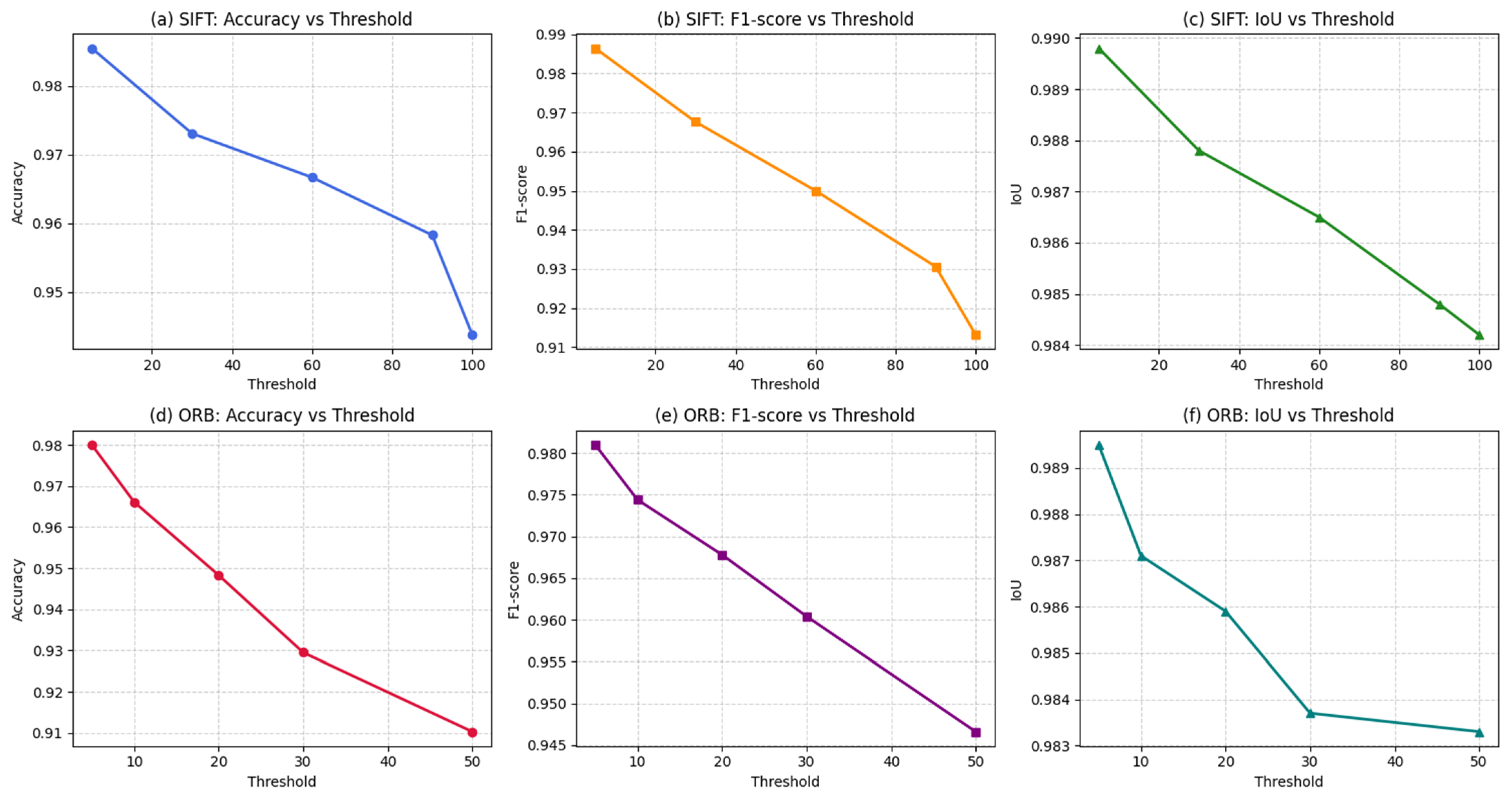
Furthermore, Figure 6 presents the sensitivity analysis of the proposed tamper localization framework by treating the applied threshold levels as representative tampering rate, that is, progressively increasing degrees of manipulation severity. The threshold was selected in a data-driven manner through sensitivity analysis by examining accuracy, F1-score, and IoU over multiple threshold settings, and the final value was chosen as the operating point yielding the best overall performance. In this context, a higher threshold corresponds to a more intensive tampering condition, allowing the robustness of the method to be evaluated under increasingly challenging attack scenarios. The results show a clear monotonic decline in accuracy, F1-score, and IoU for both SIFT- and ORB-based matching as the tampering rate increases, which confirms that localization performance is inversely related to manipulation severity. For the SIFT-based case, accuracy decreases from 0.9855 at a tampering rate of 5% to 0.9438 at 100%, while the F1-score drops from 0.9864 to 0.9132; similarly, IoU shows a slight but consistent reduction from 0.9898 to 0.9842. In the ORB-based case, accuracy declines from 0.9800 to 0.9103, F1-score from 0.9810 to 0.9466, and IoU from 0.9895 to 0.9833 as the tampering rate increases from 5% to 50%.

As the tampering becomes larger or more severe, it becomes harder to match the image features correctly and to mark the exact tampered region. Because of this, the localization performance gradually decreases. However, the decrease is smooth, not sudden, and the IoU values remain very high for all tampering rate settings. This shows that the proposed method can still identify the tampered region quite accurately even when the manipulation becomes stronger. Overall, these results show that the threshold can be considered as a measure of tampering rate, and the proposed method remains reliable over a wide range of tampering levels.

4.4. Robustness Against TITO

The proposed scheme leverages keypoints correspondences and analyzes metrics such as average Euclidean distance, standard deviation of matched keypoints, the number and percentage of strong matches, and homography residuals.

• Average Euclidean distance:

$$\overline{d}={\displaystyle \frac{1}{N}}\sum _{i=1}^N{distance}_i$$

(37)

where $\overline{d}$ is the mean distance, $N$ is the total number of matched pairs, and ${distance}_i={\parallel d_i^{\left(1\right)}-d_i^{(2)}\parallel }_2$. ${\parallel . \parallel }_2$ denotes L2 norm. This metric provides a single scalar value that indicates how closely the descriptors from two images match on average.

2.

Standard deviation distances:

$${\sigma }_d=\sqrt{{\displaystyle \frac{1}{N}}\sum _{i-1}^N{({distance}_i-\overline{d})}^2}$$

(38)

A lower ${\sigma }_d$ suggests that the matches are consistently similar, whereas a higher ${\sigma }_d$ implies variability in matching quality, possibly due to geometric distortion or noise.

3.

The number and percentage of strong matches:

$$p_{good}=\left({\displaystyle \frac{\left|\mathcal{G}\right|}{\left|\mathcal{M}\right|}}\right)\times 100.$$

(39)

$\left|\mathcal{G}\right|$ is the number of good matches, and $\left|\mathcal{M}\right|$ is the total number of matches. The percentage indicates how many of the detected matches are reliable.

4.

Homography residual:

When detecting tampering between two images that might be geometrically transformed, it is essential to understand how one image relates spatially to the other. This is done using homography estimation, which determines a transformation that aligns corresponding points between the images. First, extract the spatial coordinates of keypoints involved in “good” feature matches between $I_O$ and $I_w$, where $P_i^{(1)}=(x_i^{\left(1\right)},y_i^{\left(1\right)})$ from $I_O$ and $P_i^{(2)}=(x_i^{\left(2\right)},y_i^{\left(2\right)})$ from $I_w$.

Then, a homography is a $3\times 3$ matrix $H$ that relates the coordinates of corresponding points between two planes.

$$\left[\begin{array}{c}{x}^{(2)}\\ y^{(2)}\\ 1\end{array}\right]~H\left[\begin{array}{c}{x}^{(1)}\\ y^{(1)}\\ 1\end{array}\right]$$

(40)

Table 12. Tamper detection analysis for the rotated images.

Image	SIFT
$I_{RGB}^{16}$ Rotation (135$°$)	$\mathcal{T}=100\%$	$\mathcal{T}=90\%$	$\mathcal{T}=60\%$	$\mathcal{T}=30\%$	$\mathcal{T}=5\%$
	ORB
	$\mathcal{T}=50\%$	$\mathcal{T}=30\%$	$\mathcal{T}=20\%$	$\mathcal{T}=10\%$	$\mathcal{T}=5\%$
	SIFT
$I_{RGB}^{16}$ Rotation (45$°$)	$\mathcal{T}=100\%$	$\mathcal{T}=90\%$	$\mathcal{T}=60\%$	$\mathcal{T}=30\%$	$\mathcal{T}=5\%$
	ORB
	$\mathcal{T}=50\%$	$\mathcal{T}=30\%$	$\mathcal{T}=20\%$	$\mathcal{T}=10\%$	$\mathcal{T}=5\%$
	SIFT
$I_{RGB}^{16}$ Rotation (90$°$)	$\mathcal{T}=100\%$	$\mathcal{T}=90\%$	$\mathcal{T}=60\%$	$\mathcal{T}=30\%$	$\mathcal{T}=5\%$
	ORB
	$\mathcal{T}=50\%$	$\mathcal{T}=30\%$	$\mathcal{T}=20\%$	$\mathcal{T}=10\%$	$\mathcal{T}=5\%$
	SIFT
$I_{RGB}^{17}$ Rotation (10$°$)	$\mathcal{T}=100\%$	$\mathcal{T}=90\%$	$\mathcal{T}=60\%$	$\mathcal{T}=30\%$	$\mathcal{T}=5\%$
	ORB
	$\mathcal{T}=50\%$	$\mathcal{T}=30\%$	$\mathcal{T}=20\%$	$\mathcal{T}=10\%$	$\mathcal{T}=5\%$
	SIFT
$I_{RGB}^{20}$ Rotation (30$°$)	$\mathcal{T}=100\%$	$\mathcal{T}=90\%$	$\mathcal{T}=60\%$	$\mathcal{T}=30\%$	$\mathcal{T}=5\%$
	ORB
	$\mathcal{T}=50\%$	$\mathcal{T}=30\%$	$\mathcal{T}=20\%$	$\mathcal{T}=10\%$	$\mathcal{T}=5\%$

represents the SIFT and ORB tamper detection between the rotated images of 135$°$, 45$°$, 90$°$, 10$°$, and 30$°$.

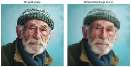
The structure and results of Table 9 and Table 12 are largely similar especially in terms of the original image and rotation (45$°$), indicating consistent detection patterns. It can be observed that SIFT consistently detects tampered regions of the background and the subject, whereas ORB detects tampered regions particularly of the focused subject. The similarity between the two tables affirms the rotation invariance capability of SIFT and ORB, making them more reliable for forensic tasks involving geometric transformations. Furthermore,

Table 13. Overview of performance metrics.

Original Images
Images	$\overline{\mathit{d}}$	${\mathsf{\sigma }}_{\mathit{d}}$	${\mathit{p}}_{\mathit{g}\mathit{o}\mathit{o}\mathit{d}}$	$\mathit{H}$
$I_{RGB}^1$	67.4	54.4	71.90%
$I_{RGB}^2$	66.4	55.6	73.54%
$I_{RGB}^3$	66.5	55.3	72.45%
$I_{RGB}^4$	68.8	55.6	75.88%
$I_{RGB}^5$	64.7	55.9	74.82%
$I_{RGB}^6$	63.9	54.3	72.89%
$I_{RGB}^7$	64.7	56.3	72.78%
$I_{RGB}^8$	64.8	55.2	73.80%
$I_{RGB}^9$	66.2	54.8	73.70%
$I_{RGB}^{10}$	67.4	54.5	73.60%
$I_{RGB}^{11}$	65.3	55.1	71.78%
$I_{RGB}^{12}$	65.4	55.2	71.92%
$I_{RGB}^{13}$	65.3	55.7	72.99%
$I_{RGB}^{14}$	66.3	56.2	72.96%
$I_{RGB}^{15}$	67.4	56.5	72.76%
$I_{RGB}^{16}$	68.3	56.3	71.87%
Rotated Images (45°)
Images	$\overline{\mathit{d}}$	${\mathsf{\sigma }}_{\mathit{d}}$	${\mathit{p}}_{\mathit{g}\mathit{o}\mathit{o}\mathit{d}}$	$\mathit{H}$
$I_{RGB}^1$	67.5	54.4	71.91%
$I_{RGB}^2$	66.2	55.7	73.55%
$I_{RGB}^3$	65.8	55.4	72.43%
$I_{RGB}^4$	68.7	55.5	75.86%
$I_{RGB}^5$	64.8	56.1	74.83%
$I_{RGB}^6$	63.7	54.3	72.87%
$I_{RGB}^7$	64.8	56.6	72.75%
$I_{RGB}^8$	64.5	55.5	73.79%
$I_{RGB}^9$	66.2	53.8	73.70%
$I_{RGB}^{10}$	67.4	54.6	73.61%
$I_{RGB}^{11}$	65.3	54.3	71.79%
$I_{RGB}^{12}$	65.4	55.2	71.92%
$I_{RGB}^{13}$	65.6	55.8	72.98%
$I_{RGB}^{14}$	66.4	56.2	72.90%
$I_{RGB}^{15}$	67.5	56.7	72.78%
$I_{RGB}^{16}$	68.7	56.6	71.85%

provides a comprehensive overview of the first 16 input images evaluated across various performance metrics.

It has been observed that several images such as $I_{RGB}^1$, $I_{RGB}^8$, $I_{RGB}^{11}$, $I_{RGB}^{14}$, and $I_{RGB}^{16}$ achieved similar homograph matrices which makes them similar to the rotation. The similarity between the original and the rotated image is clearly represented in Table 8. Across both conditions, the variation in $\overline{d}$ and ${\sigma }_d$ are minimal, and $p_{good}$ remains nearly identical, typically differing by less than 0.01 percentage points. These negligible deviations indicate that the system exhibits rotational invariance, maintaining consistent prediction accuracy and stability in displacement measures regardless of image orientation. This implies the robustness of the underlying algorithm to geometric transformations such as rotation. For example, $I_{RGB}^4$ shows near-identical values across conditions, with $\overline{d}$ of 68.8 (original) versus 68.7 (rotated), and a $p_{good}$ 75.88% versus 75.86%, indicating virtually no performance degradation due to rotation. Similarly, $I_{RGB}^4$ exhibits $\overline{d}$ values of 63.9 and 63.7, and $p_{good}$ drops marginally from 72.89% and 72.87%, showing excellent consistency and stability. In the case of $I_{RGB}^{14}$, the $\overline{d}$ slightly increases from 66.3 to 66.4 and $p_{good}$ drops marginally from 72.96% to 72.90% suggesting a minimal sensitivity to rotation, yet still within acceptable tolerance. Additionally,

Table 14. Number of tampered pixels based on different $\mathcal{T}$.

Image	Tampered Regions for SIFT
Original	$\mathcal{T}=100\%$                 $\mathcal{T}=90\%$                   $\mathcal{T}=60\%$                   $\mathcal{T}=30\%$                $\mathcal{T}=5\%$
	Number of tampered pixels
	27,664	13,713	8230	5295	4460
	Tampered regions for ORB
	$\mathcal{T}=50\%$                   $\mathcal{T}=30\%$                   $\mathcal{T}=20\%$                 $\mathcal{T}=10\%$                   $\mathcal{T}=5\%$
	Number of tampered pixels
	1218	757	406	174	29
Rotation (45$°$)	Tampered regions for SIFT
	$\mathcal{T}=100\%$                 $\mathcal{T}=90\%$                   $\mathcal{T}=60\%$                   $\mathcal{T}=30\%$                $\mathcal{T}=5\%$
	Number of tampered pixels
	27,664	13,713	8230	5290	4465
	Tampered regions for ORB
	$\mathcal{T}=50\%$                   $\mathcal{T}=30\%$                   $\mathcal{T}=20\%$                 $\mathcal{T}=10\%$                   $\mathcal{T}=5\%$
	Number of tampered pixels
	1218	757	406	212	29

represents that the number of detected tampered pixels varies significantly with the chosen threshold. In terms of SIFT, for $\mathcal{T}=100\%$, a total of 27,664 tampered pixels were identified; similarly, for 90%, 60%, 30%, and 5%, the tampered pixels were 13,713, 8230, 5295, and 4460, respectively. For ORB, a total number of 1218 of pixels were found to be tampered with for $\mathcal{T}=50\%$. Similarly, for 30%, 20%, 10%, and 5% the subsequent numbers of tampered pixels are 757, 406, 174, and 29.

For both SIFT and ORB, the number of detected tampered pixels is reported under incremental values of $\mathcal{T}$. As expected, increasing the threshold leads to a gradual reduction in the number of detected tampered pixels, reflecting stricter matching criteria and reduced sensitivity to minor distortions. Importantly, the results show a high degree of consistency between the original and rotated images. The number of tampered pixels identified using SIFT at $\mathcal{T}=5\%$, $\mathcal{T}=30\%$, $\mathcal{T}=60\%$, $\mathcal{T}=90\%$, and $\mathcal{T}=100\%$ remains nearly identical across both versions of the image. A similar trend is observed for ORB, where the detection results are closely aligned under all threshold levels.

These findings demonstrate the robustness of both SIFT and ORB to geometric transformations, with SIFT offering higher sensitivity and detecting more tampered pixels and ORB providing a more conservative, precision-oriented detection. This invariance to rotation validates their suitability for tamper detection in scenarios where images may undergo geometric transformations during unauthorized manipulation.

4.5. Computational Complexity Analysis

The computational complexity of the proposed color image watermarking framework is examined with an input image of size $N\times N$, where $N=512.$ To further quantify the computational expense, the number of floating-point operations (FLOPs) necessary for each stage is assessed for a single $512\times 512$ image and for a dataset of 24 images. Let $M=N^2=\mathrm{262,144}$, block size $b=8$, and the number of blocks $B={\left(N/b\right)}^2=4096$.

Table 15. Computational complexity and approximate FLOP analysis of the proposed watermarking framework for one image and 24 images.

Stage	Main Operation	Big-O Complexity	Approximate FLOPs/Operations Per Image	Approximate FLOPs/Operations for 24 Images
Watermark fusion	LSB embedding of biometrics into signature	$O\left(N^2\right)$	$2.62\times {10}^5$	$6.29\times {10}^6$
DWT	One-level 2D DWT	$O\left(N^2\right)$	$2.10\times {10}^6$	$5.04\times {10}^7$
DCT	Block-wise $4\times 4$DCT	$O\left(N^2\right)$	$2.62\times {10}^6$	$6.29\times {10}^7$
SVD	Block-wise $4\times 4$SVD	$O\left(N^2\right)$	$8.39\times {10}^7$	$2.01\times {10}^9$
Core embedding total	Fusion + DWT + DCT + SVD	$O\left(N^2\right)$	$8.9\times {10}^7$	$2.14\times {10}^9$
SIFT extraction	Scale-space extrema + descriptors	$\approx O\left(N^2\right)$	$5.31\times {10}^6$	$1.27\times {10}^8$
ORB extraction	FAST keypoints + BRIEF descriptor	$\approx O\left(N^2\right)$	$2.64\times {10}^6$	$6.34\times {10}^7$
Total with feature extraction	Core embedding + SIFT + ORB	$O\left(N^2\right)$	$9.7\times {10}^7$	$2.33\times {10}^9$
Descriptor matching	SIFT + ORB matching	$O\left(K^2\right)$	$4.0\times {10}^7$	$9.6\times {10}^8$
Grand total	Full pipeline including matching	$O\left(N^2\right)+O\left(K^2\right)$	$\mathbf{1.37}\times {\mathbf{10}}^{\mathbf{8}}$	$\mathbf{3.29}\times {\mathbf{10}}^{\mathbf{9}}$

shows the complexity and approximate FLOP analysis of the proposed watermarking framework.

In summary, the complexity and FLOP analysis verifies that the proposed watermarking architecture sustains a reasonable computational expense while providing improved robustness and tamper detection efficacy. The experimental design indicates that the primary computational load originates from the SVD-based embedding phase, whereas the subsequent stages contribute just a modest cost. Nonetheless, the overall complexity remains manageable for $512\times 512$ images and scales predictably with the quantity of incoming images.

4.6. Execution Time Analysis

Table 16. Execution time analysis in seconds (s).

Images	Watermark Fusion	Embedding	Extraction	Watermark Decoupling	Tamper Detection
					SIFT Descriptors	ORB Descriptors
$I_{RGB}^1$	0.0456 s	1.2456 s	1.2348 s	0.0372 s	2.2348 s	2.2435 s
$I_{RGB}^2$	0.0456 s	1.1375 s	1.1567 s	0.0372 s	2.2323 s	2.2230 s
$I_{RGB}^3$	0.0456 s	1.2344 s	1.2410 s	0.0372 s	2.2412 s	2.2410 s
$I_{RGB}^4$	0.0456 s	1.2435 s	1.2422 s	0.0372 s	2.2230 s	2.2322 s
$I_{RGB}^5$	0.0456 s	1.2233 s	1.2198 s	0.0372 s	2.2413 s	2.2419 s
$I_{RGB}^6$	0.0456 s	1.2324 s	1.2219 s	0.0372 s	2.2314 s	2.2344 s
$I_{RGB}^7$	0.0456 s	1.2250 s	1.2350 s	0.0372 s	2.2267 s	2.2254 s
$I_{RGB}^8$	0.0456 s	1.2340 s	1.2232 s	0.0372 s	2.2319 s	2.2378 s
$I_{RGB}^9$	0.0456 s	1.2321 s	1.2319 s	0.0372 s	2.2412 s	2.2314 s
$I_{RGB}^{10}$	0.0456 s	1.2111 s	1.2123 s	0.0372 s	2.2333 s	2.2340 s
$I_{RGB}^{11}$	0.0456 s	1.2011 s	1.2043 s	0.0372 s	2.2210 s	2.2212 s
$I_{RGB}^{12}$	0.0456 s	1.1578 s	1.1892 s	0.0372 s	2.2421 s	2.2322 s
$I_{RGB}^{13}$	0.0456 s	1.1873 s	1.2010 s	0.0372 s	2.2219 s	2.2221 s
$I_{RGB}^{14}$	0.0456 s	1.1922 s	1.1948 s	0.0372 s	2.2329 s	2.2319 s
$I_{RGB}^{15}$	0.0456 s	1.1878 s	1.1880 s	0.0372 s	2.2444 s	2.2410 s
$I_{RGB}^{16}$	0.0456 s	1.1901 s	1.1916 s	0.0372 s	2.2350 s	2.2344 s
$I_{RGB}^{17}$	0.0456 s	1.2240 s	1.2132 s	0.0372 s	2.2419 s	2.2414 s
$I_{RGB}^{18}$	0.0456 s	1.2221 s	1.2219 s	0.0372 s	2.2512 s	2.2440 s
$I_{RGB}^{19}$	0.0456 s	1.2011 s	1.2023 s	0.0372 s	2.2433 s	2.2312 s
$I_{RGB}^{20}$	0.0456 s	1.1911 s	1.1943 s	0.0372 s	2.2310 s	2.2422 s
$I_{RGB}^{21}$	0.0456 s	1.1478 s	1.1792 s	0.0372 s	2.2521 s	2.2321 s
$I_{RGB}^{22}$	0.0456 s	1.1773 s	1.1910 s	0.0372 s	2.2319 s	2.2419 s
$I_{RGB}^{23}$	0.0456 s	1.1822 s	1.1848 s	0.0372 s	2.2429 s	2.2510 s
$I_{RGB}^{24}$	0.0456 s	1.1778 s	1.1780 s	0.0372 s	2.2544 s	2.2444 s

delineates the runtime analysis of the proposed methodology for 16 RGB input images. Since the proposed method is designed for offline forensic and image authentication applications, processing times on the order of seconds are acceptable for the targeted use-case.

The findings indicate that watermark fusion and watermark decoupling necessitate minimal processing time, consistently recorded at 0.0456 s and 0.0372 s, respectively, across all images. The similar runtime signifies that these phases are rapid, stable, and efficient, continually operating without creating any bit errors. The embedding and extraction demonstrate marginally elevated runtimes, typically ranging from about 1.13 s to 1.25 s signifying consistent computational efficiency across diverse inputs. Both feature-based techniques for tamper detection necessitate a rather extended duration, with SIFT descriptors requiring approximately 2.22–2.24 s and ORB descriptors both lasting about 2.22–2.24 s.

Overall, the table represents that the proposed technique exhibits uniform runtime performance across all test images, with tamper detection being the most time-intensive phase.

4.7. Comparative Analysis with State-of-the-Art Methods

To validate the effectiveness and robustness of the proposed method, a series of experiments are conducted and the results are benchmarked against several existing techniques reported in the literature, including both grayscale- and color-image-based watermarking approaches. Particular attention is given to recent SIFT-based methods, enabling a focused comparison in terms of perceptual transparency. The following subsections detail the comparative analysis and insights derived from the obtained details.

• Benchmarking against gray image watermarking techniques:

Table 17. PSNR (dB) comparison with the existing grayscale techniques with Refs. [23,24,28,34].

$I_{RGB}^1$	$I_{RGB}^2$
$I_{RGB}^3$	$I_{RGB}^4$
$I_{RGB}^5$	$I_{RGB}^6$

shows the comparison in terms of PSNR. To illustrate the implementation process, a sequence of cover images $I_{RGB}^1{, I}_{RGB}^2$, $I_{RGB}^3$, $I_{RGB}^4$, $I_{RGB}^5$, and $I_{RGB}^6$ is utilized that collectively captures the progression of visual data over time, offering a clear and structured visualization of the underlying method.

Table 12 represents that, in terms of $I_{RGB}^1$, Gull et al. [23] achieved a PSNR of 51.32 dB, while methods proposed in [24,28,34] reported PSNR values of 42.44, 43.45, and 51.25 dB, respectively. The proposed scheme outperforms all the existing techniques with a PSNR of 55.34 dB. Similarly, for $I_{RGB}^2$, $I_{RGB}^3$, $I_{RGB}^4$, $I_{RGB}^5$, and $I_{RGB}^6$, the proposed technique demonstrates greater robustness compared to the existing ones.

• Comparison of the efficacy against numerous attacks with the existing gray image watermarking techniques:

Table 18. Average PSNR (dB) and SSIM comparison against numerous image processing attacks with the existing gray image watermarking techniques.

Attacks	Gull et al. [23]		Swain et al. [24]		Mao et al. [28]		Rijati et al. [34]		Proposed Method
	PSNR	SSIM	PSNR	SSIM	PSNR	SSIM	PSNR	SSIM	PSNR	SSIM
JPEG (compression quality of 5)	32.58	0.8850	31.46	0.8847	32.40	0.8852	31.48	0.8849	34.28	0.8995
JPEG (compression quality of 50)	29.56	0.9329	29.43	0.9333	29.44	0.9327	29.45	0.9331	30.44	0.9430
JPEG (compression quality of 70)	29.45	0.9850	29.31	0.9848	29.47	0.9855	29.33	0.9852	29.67	0.9864
JPEG (compression quality of 90)	28.32	0.9745	27.54	0.9745	28.38	0.9749	27.56	0.9747	28.87	0.9858
Median filtering ($10\times 10$ median filter)	31.22	0.9724	31.41	0.9728	31.26	0.9733	31.43	0.9726	32.32	0.9878
Rotation (10$°$)	30.27	0.9747	30.55	0.9745	30.31	0.9756	30.57	0.9749	31.45	0.9892
Rotation (30$°$)	30.25	0.9745	30.52	0.9742	30.29	0.9754	30.55	0.9747	31.09	0.9885
Rotation ($45°$)	29.63	0.9788	29.46	0.9792	29.68	0.9794	29.48	0.9790	30.42	0.9880
Rotation (90$°$)	28.52	0.9762	28.37	0.9766	28.57	0.9759	28.39	0.9764	29.86	0.9875
Rotation (135$°$)	29.45	0.9755	29.45	0.9759	29.55	0.9775	29.47	0.9757	30.33	0.9879
Downscaling (scaling factor = 0.1)	26.48	0.9622	26.51	0.9626	26.58	0.9632	26.53	0.9624	27.32	0.9781
Downscaling (scaling factor = 0.3)	26.44	0.9778	26.35	0.9782	26.46	0.9768	26.37	0.9780	27.95	0.9800
Upscaling (scaling factor = 10.0)	30.57	0.9875	30.27	0.9879	30.59	0.9885	30.29	0.9877	31.22	0.9889
Horizontal translation (shifting value = 100)	29.78	0.9745	29.49	0.9749	29.80	0.9735	29.51	0.9747	30.44	0.9895
Vertical translation (shifting value = 100)	29.75	0.9746	29.77	0.9748	29.77	0.9722	29.79	0.9750	30.65	0.9898
2D translation (horizontal shifting value = 100, vertical shifting value = 100)	29.12	0.9824	29.14	0.9826	29.14	0.9846	29.16	0.9828	29.32	0.9856
Cropping (20% cropped from each side)	29.59	0.9789	29.63	0.9791	29.68	0.9794	29.61	0.9793	30.25	0.9888
Gaussian noise (mean = 0, sigma = 35)	27.26	0.9659	27.55	0.9661	27.31	0.9666	27.28	0.9663	28. 15	0.9730
Content removal	26.45	0.9637	26.67	0.9639	26.55	0.9648	26.47	0.9641	27.17	0.9779
Histogram equalization	25.12	0.9727	25.14	0.9729	25.27	0.9735	25.23	0.9731	25. 28	0.9780

illustrates the average PSNR (dB) and SSIM metrics in relation to various image processing attacks, juxtaposed with current methodologies. It is observed that Gull et al. [23], Swain et al. [24], Mao et al. [28], and Rijati et al. [34] effectively documented the highest PSNR in JPEG (compression quality of 5) as 32.58, 31.46, 32.40, and 31.48 dB, respectively, whereas the proposed method attained a remarkable PSNR of 34.28, above all current methods.

The proposed technique achieved a minimum PSNR of 25.28 dB, which, despite being lower than that of histogram equalization, remains superior to the results in references [23,24,28,34]. However, the difference is minimal, but it significantly enhances security against histogram equalization.

• Benchmarking against CIW techniques:

Table 19. PSNR and SSIM comparison of CIW techniques.

For $\mathit{\mu }\mathbf{=}\mathbf{0.01}$
Images	Cheema et al. [43]		Chen et al. [53]		Mehraj et al. [54]		Altaf et al. [50]		Proposed Technique
	PSNR (dB)	SSIM	PSNR (dB)	SSIM	PSNR (dB)	SSIM	PSNR (dB)	SSIM	PSNR (dB)	SSIM
$I_{RGB}^7$	42.45	0.9989	40.31	0.9898	42.45	0.9990	43.23	0.9890	55.19	0.9988
$I_{RGB}^{\mathbf{8}}$	42.73	0.9986	40.44	0.9890	42.37	0.9987	43.25	0.9889	55.21	0.9990
$I_{RGB}^{\mathbf{9}}$	42.46	0.9987	40.34	0.9899	42.41	0.9989	43.27	0.9888	55.25	0.9991
$I_{RGB}^{\mathbf{10}}$	42.53	0.9985	40.23	0.9887	42.39	0.9992	43.24	0.9891	55.23	0.9987
$I_{RGB}^{\mathbf{11}}$	42.80	0.9984	40.13	0.9888	42.40	0.9989	43.26	0.9892	55.20	0.9990
For $\mathit{\mu }\mathbf{=}\mathbf{0.02}$
Images	Cheema et al. [43]		Chen et al. [53]		Mehraj et al. [54]		Altaf et al. [50]		Proposed technique
	PSNR (dB)	SSIM	PSNR (dB)	SSIM	PSNR (dB)	SSIM	PSNR (dB)	SSIM	PSNR (dB)	SSIM
$I_{RGB}^7$	42.45	0.9989	40.31	0.9898	42.45	0.9990	43.23	0.9890	53.10	0.9887
$I_{RGB}^{\mathbf{8}}$	42.73	0.9986	40.44	0.9890	42.37	0.9987	43.25	0.9889	53.12	0.9891
$I_{RGB}^{\mathbf{9}}$	42.46	0.9987	40.34	0.9899	42.41	0.9989	43.27	0.9888	53.16	0.9890
$I_{RGB}^{\mathbf{10}}$	42.53	0.9985	40.23	0.9887	42.39	0.9992	43.24	0.9891	53.14	0.9886
$I_{RGB}^{\mathbf{11}}$	42.80	0.9984	40.13	0.9888	42.40	0.9989	43.26	0.9892	53.11	0.9889
For $\mathit{\mu }\mathbf{=}\mathbf{0.03}$
Images	Cheema et al. [43]		Chen et al. [53]		Mehraj et al. [54]		Altaf et al. [50]		Proposed technique
	PSNR (dB)	SSIM	PSNR (dB)	SSIM	PSNR (dB)	SSIM	PSNR (dB)	SSIM	PSNR (dB)	SSIM
$I_{RGB}^7$	42.45	0.9989	40.31	0.9898	42.45	0.9990	43.23	0.9890	51.32	0.9878
$I_{RGB}^{\mathbf{8}}$	42.73	0.9986	40.44	0.9890	42.37	0.9987	43.25	0.9889	51.34	0.9882
$I_{RGB}^{\mathbf{9}}$	42.46	0.9987	40.34	0.9899	42.41	0.9989	43.27	0.9888	51.38	0.9881
$I_{RGB}^{\mathbf{10}}$	42.53	0.9985	40.23	0.9887	42.39	0.9992	43.24	0.9891	51.36	0.9877
$I_{RGB}^{\mathbf{11}}$	42.80	0.9984	40.13	0.9888	42.40	0.9989	43.26	0.9892	51.33	0.9880
For $\mathit{\mu }\mathbf{=}\mathbf{0.04}$
Images	Cheema et al. [43]		Chen et al. [53]		Mehraj et al. [54]		Altaf et al. [50]		Proposed technique
	PSNR (dB)	SSIM	PSNR (dB)	SSIM	PSNR (dB)	SSIM	PSNR (dB)	SSIM	PSNR (dB)	SSIM
$I_{RGB}^7$	42.45	0.9989	40.31	0.9898	42.45	0.9990	43.23	0.9890	50.51	0.9867
$I_{RGB}^{\mathbf{8}}$	42.73	0.9986	40.44	0.9890	42.37	0.9987	43.25	0.9889	50.53	0.9871
$I_{RGB}^{\mathbf{9}}$	42.46	0.9987	40.34	0.9899	42.41	0.9989	43.27	0.9888	50.57	0.9870
$I_{RGB}^{\mathbf{10}}$	42.53	0.9985	40.23	0.9887	42.39	0.9992	43.24	0.9891	50.55	0.9866
$I_{RGB}^{\mathbf{11}}$	42.80	0.9984	40.13	0.9888	42.40	0.9989	43.26	0.9892	50.52	0.9869

demonstrates the comparative analysis in terms of PSNR and SSIM for all embedding strengths, $\mu =0.01, 0.02, 0.03$, and 0.04. Among the existing techniques, Cheema et al. [43] report the highest average SSIM values, ranging from 0.9984 to 0.9989, and maintain PSNR levels consistently above 42 dB, indicating storing imperceptibility. Mehraj et al. [54] also achieve competitive SSIM values up to 0.9992, though their PSNR remains slightly lower, around 42.37–42.45 dB. Chen et al. [53], while structurally comparable with SSIM scores nearing 0.9899, present the lowest PSNR values among the group (approximately 40.13–40.44 dB), suggesting more noticeable distortion. Altaf et al. improve on this with PSNR values in the range of 43.23–43.27 dB and SSIM between 0.9888 and 0.9892, reflecting a more balanced performance. In contrast, the proposed technique significantly surpasses the existing methods, achieving PSNR values consistently above 55 dB for $\mu =0.01$, 53 dB for $\mu =0.02$, 51 dB for $\mu =0.03$, and 50 dB for $\mu =0.04$. This substantial improvement in both fidelity and structural similarity demonstrates the effectiveness of the proposed method in maintaining visual quality and perceptual integrity while embedding watermark information.

• Comparison of the efficacy against numerous attacks with the existing color image watermarking techniques:

Table 20. Average PSNR (dB) and SSIM comparison against numerous image processing attacks with the existing color image watermarking techniques.

Attacks	Cheema et al. [43]		Chen et al. [53]		Mehraj et al. [54]		Altaf et al. [50]		Proposed Method
	PSNR	SSIM	PSNR	SSIM	PSNR	SSIM	PSNR	SSIM	PSNR	SSIM
JPEG (compression quality of 5)	32.48	0.8845	32.55	0.8848	32.46	0.8847	32.50	0.8843	34.28	0.8995
JPEG (compression quality of 50)	29.24	0.9334	29.27	0.9337	29.26	0.9336	29.22	0.9332	30.44	0.9430
JPEG (compression quality of 70)	29.25	0.9845	29.28	0.9848	29.27	0.9847	29.23	0.9843	29.67	0.9864
JPEG (compression quality of 90)	28.22	0.9740	28.25	0.9743	28.24	0.9742	28.20	0.9738	28.87	0.9858
Median filtering ($10\times 10$ median filter)	31.12	0.9719	31.15	0.9722	31.14	0.9721	31.10	0.9717	32.32	0.9878
Rotation (10$°$)	30.17	0.9742	30.20	0.9745	30.19	0.9740	30.15	0.9740	31.45	0.9892
Rotation (30$°$)	30.12	0.9740	30.18	0.9742	30.17	0.9738	30.13	0.9738	31.09	0.9885
Rotation ($45°$)	29.43	0.9783	29.46	0.9786	29.45	0.9781	29.41	0.9781	30.42	0.9880
Rotation (90$°$)	28.32	0.9777	28.35	0.9780	28.34	0.9779	28.30	0.9775	29.86	0.9875
Rotation (135$°$)	29.35	0.9750	29.38	0.9753	29.37	0.9752	29.33	0.9748	30.33	0.9879
Downscaling (scaling factor = 0.1)	26.28	0.9617	26.31	0.9620	26.30	0.9619	26.26	0.9615	27.32	0.9781
Downscaling (scaling factor = 0.3)	26.24	0.9773	26.27	0.9776	26.26	0.9775	26.22	0.9771	27.95	0.9800
Upscaling (scaling factor = 10.0)	30.37	0.9870	30.40	0.9873	30.39	0.9872	30.35	0.9868	31.22	0.9889
Horizontal translation (shifting value = 100)	29.58	0.9740	29.51	0.9738	29.60	0.9742	29.56	0.9738	30.44	0.9895
Vertical translation (shifting value = 100)	29.55	0.9741	29.48	0.9748	29.57	0.9743	29.53	0.9739	30.65	0.9898
2D translation (horizontal shifting value = 100, vertical shifting value = 100)	29.05	0.9819	29.08	0.9826	29.07	0.9821	29.03	0.9817	29.32	0.9856
Cropping (20% cropped from each side)	29.39	0.9784	29.42	0.9790	29.41	0.9786	29.37	0.9782	30.25	0.9888
Gaussian noise (mean = 0, sigma = 35)	27.16	0.9654	27.19	0.9658	27.18	0.9652	27.14	0.9652	28. 15	0.9730
Content removal	26.25	0.9632	26.28	0.9635	26.27	0.9630	26.23	0.9630	27.17	0.9779
Histogram equalization	25.02	0.9722	25.05	0.9725	25.04	0.9720	25.00	0.9718	25.28	0.9780

exhibits the average PSNR (dB) and SSIM comparisons across several image processing attacks for the existing color image watermarking techniques. The observation reveals that references [33,43,50,54] report the highest PSNR value against JPEG (compression quality of 5) as 32.48, 32.55, 32.46, and 32.50, respectively. However, when the compression quality increases, the PSNR and SSIM values diminish.

Conversely, a small distortion of 0.28 in PSNR is detected between the proposed technique and references [43,50,53,54] as compared to histogram equalization.

• Benchmarking against SIFT-based watermarking techniques:

Table 21. PSNR and SSIM comparison for SIFT watermarking.

For $\mathit{\mu }\mathbf{=}\mathbf{0.01}$
Images	Hamidi et al. [56]		Gan et al. [59]		Proposed Technique
	PSNR (dB)	SSIM	PSNR (dB)	SSIM	PSNR (dB)	SSIM
$I_{RGB}^{12}$	48.95	0.9995	42.64	0.9874	55.15	0.9899
$I_{RGB}^{\mathbf{13}}$	48.96	0.9997	42.65	0.9879	55.16	0.9993
$I_{RGB}^{\mathbf{14}}$	48.97	0.9996	42.62	0.9876	55.31	0.9996
$I_{RGB}^{\mathbf{15}}$	48.94	0.9998	42.63	0.9877	55.30	0.9994
$I_{RGB}^{\mathbf{16}}$	48.94	0.9997	42.60	0.9878	55.27	0.9997
For $\mathit{\mu }\mathbf{=}\mathbf{0.02}$
Images	Hamidi et al. [56]		Gan et al. [59]		Proposed technique
	PSNR (dB)	SSIM	PSNR (dB)	SSIM	PSNR (dB)	SSIM
$I_{RGB}^{12}$	48.95	0.9995	42.64	0.9874	53.06	0.9798
$I_{RGB}^{\mathbf{13}}$	48.96	0.9997	42.65	0.9879	53.07	0.9892
$I_{RGB}^{\mathbf{14}}$	48.97	0.9996	42.62	0.9876	53.22	0.9895
$I_{RGB}^{\mathbf{15}}$	48.94	0.9998	42.63	0.9877	53.21	0.9893
$I_{RGB}^{\mathbf{16}}$	48.94	0.9997	42.60	0.9878	53.18	0.9896
For $\mathit{\mu }\mathbf{=}\mathbf{0.03}$
Images	Hamidi et al. [56]		Gan et al. [59]		Proposed technique
	PSNR (dB)	SSIM	PSNR (dB)	SSIM	PSNR (dB)	SSIM
$I_{RGB}^{12}$	48.95	0.9995	42.64	0.9874	51.28	0.9789
$I_{RGB}^{\mathbf{13}}$	48.96	0.9997	42.65	0.9879	51.29	0.9883
$I_{RGB}^{\mathbf{14}}$	48.97	0.9996	42.62	0.9876	51.44	0.9886
$I_{RGB}^{\mathbf{15}}$	48.94	0.9998	42.63	0.9877	51.43	0.9884
$I_{RGB}^{\mathbf{16}}$	48.94	0.9997	42.60	0.9878	51.40	0.9887
For $\mathit{\mu }\mathbf{=}\mathbf{0.04}$
Images	Hamidi et al. [56]		Gan et al. [59]		Proposed technique
	PSNR (dB)	SSIM	PSNR (dB)	SSIM	PSNR (dB)	SSIM
$I_{RGB}^{12}$	48.95	0.9995	42.64	0.9874	50.47	0.9778
$I_{RGB}^{\mathbf{13}}$	48.96	0.9997	42.65	0.9879	50.48	0.9872
$I_{RGB}^{\mathbf{14}}$	48.97	0.9996	42.62	0.9876	50.63	0.9875
$I_{RGB}^{\mathbf{15}}$	48.94	0.9998	42.63	0.9877	50.62	0.9873
$I_{RGB}^{\mathbf{16}}$	48.94	0.9997	42.60	0.9878	50.61	0.9876

summarizes the comparative performance of the watermarking techniques with respect to $\mu =0.01, 0.02, 0.03,$ and 0.04. Hamidi et al. [56]’s method demonstrates strong fidelity with PSNR values around 48.95 dB and SSIM values nearing 0.9998, reflecting high imperceptibility. However, the method by Gan et al. [59], while acceptable in performance, shows relatively lower PSNR (approximately 42.60–42.65 dB) and SSIM (around 0.9874–0.9879), indicating perceptual degradation. The proposed technique exhibits a substantial gain in both robustness and perceptual quality, with the highest PSNR and SSIM for $\mu =0.01$, 0,02, 0.03, and 0.04, confirming its superiority in preserving image visibility after watermark embedding.

• Comparison of tamper detection analysis against the SIFT-based watermarking techniques:

Table 22. Average accuracy, precision, and MCC comparison on SIFT.

$\mathcal{T}$	Hamidi et al. [56]			Gan et al. [59]			Proposed Technique
	Accuracy	Precision	MCC	Accuracy	Precision	MCC	Accuracy	Precision	MCC
5%	0.9754	0.9748	0.9610	0.9762	0.9751	0.9625	0.9855	0.9813	0.9706
30%	0.9538	0.9529	0.9215	0.9547	0.9537	0.9238	0.9731	0.9661	0.9320
60%	0.9368	0.9357	0.8826	0.9375	0.9368	0.8871	0.9667	0.9597	0.8963
90%	0.9098	0.9084	0.8431	0.9102	0.9098	0.8442	0.9583	0.9529	0.8522
100%	0.8948	0.8967	0.8157	0.8978	0.8981	0.8175	0.9438	0.9374	0.8203

compares the average tamper detection performance of the proposed technique with those of Hamidi et al. [56] and Gan et al. [59] for different values of $\mathcal{T}$. It can be observed that, although the performance of all methods gradually decreases as $\mathcal{T}$ increases, the proposed technique consistently achieves the highest accuracy, precision and MCC across all tested values of $\mathcal{T}$. For example, at $\mathcal{T}=5\%$, the proposed technique attains an average accuracy of 0.9855, a precision of 0.9813, and MCC of 0.9706, which are higher than the corresponding values of the compared methods. Even at larger values such as $\mathcal{T}=100\%$, the proposed method maintains superior performance, demonstrating its effectiveness and robustness for tamper detection.

• Benchmarking against DWT-DCT-SVD-based watermarking techniques:

Table 23. PSNR, SSIM, and NCC comparison of DWT-DCT-SVD techniques.

Images	Awasthi et al. [60]		Devi et al. [61]		Arora et al. [62]			Varghese et al. [63]		Proposed Technique
	PSNR (dB)	NCC	PSNR (dB)	NCC	PSNR (dB)	SSIM	NCC	PSNR (dB)	SSIM	PSNR (dB)	SSIM	NCC
$I_{RGB}^1$	44.95	0.9682	47.32	0.9678	55.21	0.9798	0.9691	43.34	0.9792	55.34	0.9999	0.9781
$I_{RGB}^2$	44.65	0.9781	47.45	0.9778	55.02	0.9794	0.9772	43.26	0.9777	55.23	0.9895	0.9882
$I_{RGB}^3$	44.83	0.9691	47.12	0.9689	55.11	0.9797	0.9682	43.37	0.9782	55.23	0.9898	0.9792
$I_{RGB}^4$	44.46	0.9694	47.29	0.9688	55.05	0.9791	0.9685	43.28	0.9787	55.13	0.9992	0.9795
$I_{RGB}^5$	44.37	0.9797	47.30	0.9789	55.08	0.9794	0.9788	43.29	0.9753	55.10	0.9995	0.9898
$I_{RGB}^6$	44.24	0.9790	47.41	0.9789	55.15	0.9797	0.9781	43.35	0.9797	55.29	0.9998	0.9891
$I_{RGB}^7$	44.58	0.9794	47.32	0.9787	55.09	0.9787	0.9785	43.31	0.9772	55.19	0.9988	0.9895
$I_{RGB}^8$	45.33	0.9701	47.49	0.9698	55.00	0.9789	0.9692	43.40	0.9777	55.21	0.9990	0.9802
$I_{RGB}^9$	44.24	0.9691	47.23	0.9689	55.13	0.9790	0.9682	43.47	0.9763	55.25	0.9991	0.9792
$I_{RGB}^{10}$	44.38	0.9694	47.46	0.9687	55.07	0.9786	0.9685	43.33	0.9787	55.23	0.9987	0.9795
$I_{RGB}^{11}$	44.47	0.9781	47.39	0.9779	55.03	0.9789	0.9772	43.38	0.9767	55.20	0.9990	0.9882
$I_{RGB}^{12}$	44.25	0.9797	47.40	0.9788	55.05	0.9798	0.9788	43.24	0.9772	55.15	0.9899	0.9898
$I_{RGB}^{13}$	44.37	0.9800	47.37	0.9795	55.09	0.9792	0.9791	43.27	0.9787	55.16	0.9993	0.9901
$I_{RGB}^{14}$	44.29	0.9693	47.43	0.9689	55.12	0.9795	0.9684	43.21	0.9762	55.31	0.9996	0.9794
$I_{RGB}^{15}$	44.98	0.9696	47.44	0.9688	55.14	0.9793	0.9687	43.22	0.9777	55.30	0.9994	0.9797
$I_{RGB}^{16}$	44.78	0.9779	47.37	0.9770	55.14	0.9796	0.9750	43.20	0.9783	55.27	0.9997	0.9880
$I_{RGB}^{17}$	45.32	0.9690	47.22	0.9688	55.12	0.9790	0.9681	43.43	0.9786	55.19	0.9987	0.9883
$I_{RGB}^{18}$	44.23	0.9693	47.45	0.9686	55.07	0.9785	0.9684	43.32	0.9766	55.21	0.9991	0.9889
$I_{RGB}^{19}$	44.37	0.9780	47.38	0.9778	55.05	0.9788	0.9771	43.37	0.9771	55.15	0.9989	0.9887
$I_{RGB}^{20}$	44.46	0.9796	47.39	0.9787	55.06	0.9795	0.9787	43.23	0.9786	55.27	0.9990	0.9888
$I_{RGB}^{21}$	44.24	0.9798	47.38	0.9793	55.08	0.9791	0.9788	43.26	0.9761	55.30	0.9991	0.9882
$I_{RGB}^{22}$	44.36	0.9692	47.42	0.9688	55.11	0.9794	0.9683	43.20	0.9776	55.26	0.9992	0.9878
$I_{RGB}^{23}$	44.28	0.9695	47.43	0.9687	55.13	0.9792	0.9686	43.21	0.9782	55.28	0.9994	0.9880
$I_{RGB}^{24}$	44.95	0.9778	47.36	0.9770	55.13	0.9795	0.9751	43.19	0.9786	55.31	0.9993	0.9879

indicates that the proposed technique consistently surpasses the comparative methods across all input images regarding PSNR, SSIM and NCC for $\mu$ = 0.01. In comparison to Awasthi et al. [60], the proposed technique significantly enhances the PSNR, elevating it from around 44–45 dB to roughly 55 dB, hence indicating markedly improved imperceptibility of the embedded watermark. Compared to Devi et al. [61], the proposed technique demonstrates a distinct benefit, exhibiting superior PSNR and marginally improved NCC in the majority of instances, indicating enhanced fidelity and watermark recovery. While Arora et al. [62] attain commendable results, the proposed method yields marginally superior SSIM and NCC for the majority of images, signifying enhanced structural fidelity and increased resilience. Similarly, when compared to Varghese et al. [63], the proposed strategy significantly enhances the PSNR from around 43 dB to over 55 dB, while also augmenting the SSIM.

Overall, the table confirms that the proposed technique delivers the best-balanced and optimal performance among methods by maintaining image quality and facilitating dependable watermark extraction across various image samples.

4.8. Evaluation on Public Tampered Datasets

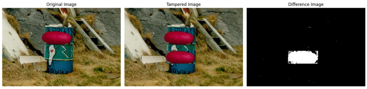
To further validate the rationality and practical applicability of the proposed tamper detection method, additional experiments were conducted on the publicly available CASIA 1.0 tampered image dataset, which contains more realistic forged images than standard test images and is widely used in image tampering detection research.

Table 24. Tampered area detection on public dataset.

Tampered image                                       Original image                                   Detected region

Tampered image                                       Original image                                   Detected region

Tampered image                                       Original image                                   Detected region

Tampered image                                       Original image                                   Detected region

Tampered image                                       Original image                                   Detected region

Tampered image                                       Original image                                   Detected region

Tampered image                                       Original image                                   Detected region

Tampered image                                       Original image                                   Detected region

Tampered image                                       Original image                                   Detected region

Tampered image                                       Original image                                   Detected region

Tampered image                                       Original image                                   Detected region

Tampered image                                       Original image                                   Detected region

Tampered image                                       Original image                                   Detected region

Tampered image                                       Original image                                   Detected region

Tampered image                                       Original image                                   Detected region

Tampered image                                       Original image                                   Detected region

Tampered image                                       Original image                                   Detected region

Tampered image                                       Original image                                   Detected region

Tampered image                                       Original image                                   Detected region

Tampered image                                       Original image                                   Detected region

presents the detected tampered regions obtained by the proposed method, showing its ability to effectively identify and localize manipulated areas under practical manipulation scenarios.

In addition,

Table 25. Tamper detection evaluation using ground-truth mask on SIFT and ORB.

SIFT
Tampering rates $\mathcal{T}$= 5%
Accuracy	Precision	MCC	Recall	F1-Score	ROC point	IOU
0.9864	0.9824	0.9715	0.9918	0.9856	0.0212, 0.9915	0.9889
Tampering rates $\mathcal{T}$= 30%
Accuracy	Precision	MCC	Recall	F1-Score	ROC point	IOU
0.9845	0.9819	0.9709	0.9910	0.9850	0.0303, 0.9922	0.9886
Tampering rates $\mathcal{T}$= 60%
Accuracy	Precision	MCC	Recall	F1-Score	ROC point	IOU
0.9736	0.9748	0.9614	0.9821	0.9743	0.0412, 0.9731	0.9879
Tampering rates $\mathcal{T}$= 90%
Accuracy	Precision	MCC	Recall	F1-Score	ROC point	IOU
0.9679	0.9688	0.9555	0.9774	0.9659	0.0511, 0.9669	0.9865
Tampering rates $\mathcal{T}$= 100%
Accuracy	Precision	MCC	Recall	F1-Score	ROC point	IOU
0.9589	0.9579	0.9465	0.9774	0.9777	0.0603, 0.9534	0.9798
ORB
Tampering rates $\mathcal{T}$= 5%
Accuracy	Precision	MCC	Recall	F1-Score	ROC point	IOU
0.9791	0.9732	0.9612	0.9857	0.9810	0.0259, 0.9835	0.9866
Tampering rates $\mathcal{T}$= 10%
Accuracy	Precision	MCC	Recall	F1-Score	ROC point	IOU
0.9683	0.9641	0.9521	0.9745	0.9765	0.0334, 0.9758	0.9732
Tampering rates $\mathcal{T}$= 20%
Accuracy	Precision	MCC	Recall	F1-Score	ROC point	IOU
0.9683	0.9641	0.9521	0.9745	0.9765	0.0334, 0.9758	0.9732
Tampering rates $\mathcal{T}$= 30%
Accuracy	Precision	MCC	Recall	F1-Score	ROC point	IOU
0.9598	0.9579	0.9487	0.9629	0.9671	0.0454, 0.9643	0.9655
Tampering rates $\mathcal{T}$= 50%
Accuracy	Precision	MCC	Recall	F1-Score	ROC point	IOU
0.9492	0.9495	0.9398	0.9596	0.9593	0.0569, 0.9597	0.9590

summarizes the tamper detection evaluation using ground-truth masks to verify the effectiveness of the proposed approach. For SIFT-based analysis, the tampering rates considered were $\mathcal{T}$ = 5%, 30%, 60%, 90%, and 100%, while for ORB-based analysis, the selected tampering rates were $\mathcal{T}$ = 5%, 10%, 20%, 30%, and 50%. The generated ground masks serve as reference masks for validating whether the detected tampered regions correspond to the actual manipulated areas. This comparison demonstrates the capability of both SIFT and ORB to support tamper detection under different levels of manipulation, with the detailed results presented in Table 25. Furthermore, Table 25 also reports the quantitative performance evaluation in terms of accuracy, precision, recall, F1-score, Matthews correlation coefficient (MCC), ROC point, and IoU. The qualitative and quantitative results together demonstrate the robustness, effectiveness, and practical relevance of the proposed method for real-world image forensic applications.

4.9. Limitations of the Proposed Technique

A key limitation of the proposed technique is its adherence to a non-blind watermarking approach. The watermark extraction process necessitates the SVD matrix S utilized during the embedding phase, as the suggested method relies on SVD-domain embedding. The reliance on original embedding-domain information constrains the practical adaptability of the system, as successful watermark recovery cannot be executed independently at the receiver without access to the necessary reference data. In real-world applications, particularly in large-scale, distributed or autonomous verification environments, it may not always be convenient to maintain and securely transmit or store this additional extraction-side information. Consequently, while the non-blind design facilitates dependable extraction and robust performance, it diminishes the general applicability of the method in comparison to fully blind watermarking techniques that retrieve the watermark without necessitating original embedding-domain components.

5. Conclusions and Future Scope

The research articulates a non-blind watermarking framework tailored for color images that effectively bridges the domains of biometric security, robust watermarking, and tamper detection under geometric transformations. The core impetus behind this work is the growing need for secure and transformation-invariant authentication in high-stakes visual data environments where integrity is paramount and content is susceptible to sophisticated manipulation. The methodological architecture comprising DWT-DCT-SVD for embedding and a fused watermark of personal signature and biometric identity is deliberately selected to enhance both robustness and imperceptibility. Furthermore, the integration of SIFT and ORB descriptors in tamper detection reflects a strategic decision to circumvent the limitations of conventional pixel-based comparison, especially under TITO. By doing so, the framework not only reinforces geometric resilience but also elevates forensic traceability. The motivation for developing such a hybrid model is deeply rooted in addressing the inadequacies of traditional watermarking systems that falter in the face of geometric misalignments or adversarial manipulation. In contrast, the proposed approach exhibits robustness not merely in terms of structural similarity or signal fidelity, but in its capacity to localize tampering with high precision and semantic context awareness.

Looking ahead, one promising trajectory is the incorporation of self-recovery mechanisms into the existing framework, enabling not just detection, but autonomous reconstruction of tampered image regions. Moreover, the convergence of quantum computing and watermarking presents an intellectually fertile frontier.

References

1. Wu, H.; Liu, G.; Yao, Y.; Zhang, X. Watermarking neural networks with watermarked images. IEEE Trans. Circuits Syst. Video Technol. 2020, 31, 2591–2601. [Google Scholar] [CrossRef]
2. Ding, W.; Ming, Y.; Cao, Z.; Lin, C.T. A generalized deep neural network approach for digital watermarking analysis. IEEE Trans. Emerg. Top. Comput. Intell. 2021, 6, 613–627. [Google Scholar] [CrossRef]
3. Wan, W.; Wang, J.; Zhang, Y.; Li, J.; Yu, H.; Sun, J. A comprehensive survey on robust image watermarking. Neurocomputing 2022, 488, 226–247. [Google Scholar] [CrossRef]
4. Zhang, J.; Chen, D.; Liao, J.; Zhang, W.; Feng, H.; Hua, G.; Yu, N. Deep model intellectual property protection via deep watermarking. IEEE Trans. Pattern Anal. Mach. Intell. 2021, 44, 4005–4020. [Google Scholar] [CrossRef] [PubMed]
5. Xie, J.; Zhao, W.; Lee, H.; Roy, D.B.; Zhang, X. Hardware circuits and systems design for post-quantum cryptography—A tutorial brief. IEEE Trans. Circuits Syst. II Express Briefs 2024, 71, 1670–1676. [Google Scholar] [CrossRef]
6. Li, Q.; Ma, B.; Fu, X.; Wang, X.; Wang, C.; Li, X. Robust Image Steganography via Color Conversion. IEEE Trans. Circuits Syst. Video Technol. 2024, 35, 1399–1408. [Google Scholar] [CrossRef]
7. Quan, Y.; Teng, H.; Chen, Y.; Ji, H. Watermarking deep neural networks in image processing. IEEE Trans. Neural Netw. Learn. Syst. 2020, 32, 1852–1865. [Google Scholar] [CrossRef]
8. Tosun, T.; Savas, E. Zero-value filtering for accelerating non-profiled side-channel attack on incomplete NTT-based implementations of lattice-based cryptography. IEEE Trans. Inf. Forensics Secur. 2024, 19, 3353–3365. [Google Scholar] [CrossRef]
9. Subramanian, N.; Elharrouss, O.; Al-Maadeed, S.; Bouridane, A. Image steganography: A review of the recent advances. IEEE Access 2021, 9, 23409–23423. [Google Scholar] [CrossRef]
10. Dhar, S.; Sahu, A.K. Digital to quantum watermarking: A journey from past to present and into the future. Comput. Sci. Rev. 2024, 54, 100679. [Google Scholar] [CrossRef]
11. Zhong, X.; Huang, P.C.; Mastorakis, S.; Shih, F.Y. An automated and robust image watermarking scheme based on deep neural networks. IEEE Trans. Multimed. 2020, 23, 1951–1961. [Google Scholar] [CrossRef]
12. Fang, H.; Chen, D.; Huang, Q.; Zhang, J.; Ma, Z.; Zhang, W.; Yu, N. Deep template-based watermarking. IEEE Trans. Circuits Syst. Video Technol. 2020, 31, 1436–1451. [Google Scholar] [CrossRef]
13. Li, Q.; Wang, X.; Ma, B.; Wang, X.; Wang, C.; Gao, S.; Shi, Y. Concealed attack for robust watermarking based on generative model and perceptual loss. IEEE Trans. Circuits Syst. Video Technol. 2021, 32, 5695–5706. [Google Scholar] [CrossRef]
14. Padhi, S.K.; Tiwari, A.; Ali, S.S. Deep Learning-based Dual Watermarking for Image Copyright Protection and Authentication. IEEE Trans. Artif. Intell. 2024, 5, 6134–6145. [Google Scholar] [CrossRef]
15. Gao, Z.; Cheng, Y.; Yin, Z. A survey of fragile model watermarking. Signal Process. 2025, 238, 110088. [Google Scholar] [CrossRef]
16. Yuan, Z.; Zhang, X.; Wang, Z.; Yin, Z. Semi-Fragile Neural Network Watermarking Based on Adversarial Examples. IEEE Trans. Emerg. Top. Comput. Intell. 2024, 8, 2775–2790. [Google Scholar] [CrossRef]
17. Wu, S.; Lu, W.; Luo, X. Robust Watermarking Based on Multi-layer Watermark Feature Fusion. IEEE Trans. Multimed. 2025, 27, 5156–5169. [Google Scholar] [CrossRef]
18. Nie, H.; Lu, S.; Wu, J.; Zhu, J. Deep model intellectual property protection with compression-resistant model watermarking. IEEE Trans. Artif. Intell. 2024, 5, 3362–3373. [Google Scholar] [CrossRef]
19. Wang, C.; Zhang, Q.; Wang, X.; Zhou, L.; Li, Q.; Xia, Z.; Ma, B.; Shi, Y.Q. Light-field image multiple reversible robust watermarking against geometric attacks. IEEE Trans. Dependable Secur. Comput. 2025, 22, 5861–5875. [Google Scholar] [CrossRef]
20. Tang, Y.; Wang, S.; Wang, C.; Xiang, S.; Cheung, Y.M. A highly robust reversible watermarking scheme using embedding optimization and rounded error compensation. IEEE Trans. Circuits Syst. Video Technol. 2022, 33, 1593–1609. [Google Scholar] [CrossRef]
21. Yan, F.; Huang, H.; Yu, X. A multi watermarking scheme for verifying medical image integrity and authenticity in the internet of medical things. IEEE Trans. Ind. Inform. 2022, 18, 8885–8894. [Google Scholar] [CrossRef]
22. Dai, Z.; Lian, C.; He, Z.; Jiang, H.; Wang, Y. A novel hybrid reversible-zero watermarking scheme to protect medical image. IEEE Access 2022, 10, 58005–58016. [Google Scholar] [CrossRef]
23. Gull, S.; Mansour, R.F.; Aljehane, N.O.; Parah, S.A. A self-embedding technique for tamper detection and localization of medical images for smart-health. Multimed. Tools Appl. 2021, 80, 29939–29964. [Google Scholar] [CrossRef]
24. Swain, M.; Swain, D. An effective watermarking technique using BTC and SVD for image authentication and quality recovery. Integration 2022, 83, 12–23. [Google Scholar] [CrossRef]
25. Aminuddin, A.; Ernawan, F.; Nincarean, D.; Amrullah, A.; Ariatmanto, D. TCBR and TCBD: Evaluation metrics for tamper coincidence problem in fragile image watermarking. Eng. Sci. Technol. Int. J. 2024, 56, 101790. [Google Scholar] [CrossRef]
26. Tang, Y.; Wang, C.; Xiang, S.; Cheung, Y.M. A robust reversible watermarking scheme using attack-simulation-based adaptive normalization and embedding. IEEE Trans. Inf. Forensics Secur. 2024, 19, 4114–4129. [Google Scholar] [CrossRef]
27. Jana, M.; Jana, B.; Joardar, S. Local feature based self-embedding fragile watermarking scheme for tampered detection and recovery utilizing AMBTC with fuzzy logic. J. King Saud Univ.-Comput. Inf. Sci. 2022, 34, 9822–9835. [Google Scholar] [CrossRef]
28. Mao, J.; Tang, H.; Lyu, S.; Zhou, Z.; Cao, X. Content-aware quantization index modulation: Leveraging data statistics for enhanced image watermarking. IEEE Trans. Inf. Forensics Secur. 2023, 19, 1935–1947. [Google Scholar] [CrossRef]
29. Lin, C.C.; Lee, T.L.; Chang, Y.F.; Shiu, P.F.; Zhang, B. Fragile watermarking for tamper localization and self-recovery based on AMBTC and VQ. Electronics 2023, 12, 415. [Google Scholar] [CrossRef]
30. Sahu, A.K. A logistic map based blind and fragile watermarking for tamper detection and localization in images. J. Ambient. Intell. Humaniz. Comput. 2022, 13, 3869–3881. [Google Scholar] [CrossRef]
31. Hussan, M.; Gull, S.; Parah, S.A.; Qureshi, G.J. An efficient encoding based watermarking technique for tamper detection and localization. Multimed. Tools Appl. 2023, 82, 37249–37271. [Google Scholar] [CrossRef]
32. Hu, R.; Xiang, S. Cover-lossless robust image watermarking against geometric deformations. IEEE Trans. Image Process. 2020, 30, 318–331. [Google Scholar] [CrossRef]
33. Bhalerao, S.; Ansari, I.A.; Kumar, A. A secure image watermarking for tamper detection and localization. J. Ambient. Intell. Humaniz. Comput. 2021, 12, 1057–1068. [Google Scholar] [CrossRef]
34. Rijati, N. Nested block based double self-embedding fragile image watermarking with super-resolution recovery. IEEE Access 2023, 11, 60939–60949. [Google Scholar] [CrossRef]
35. He, W.; Cai, Z.; Wang, Y. High-fidelity reversible image watermarking based on effective prediction error-pairs modification. IEEE Trans. Multimed. 2020, 23, 52–63. [Google Scholar] [CrossRef]
36. Ma, Z.; Zhang, W.; Fang, H.; Dong, X.; Geng, L.; Yu, N. Local geometric distortions resilient watermarking scheme based on symmetry. IEEE Trans. Circuits Syst. Video Technol. 2021, 31, 4826–4839. [Google Scholar] [CrossRef]
37. Zhang, F.; Wang, H.; He, M.; Xia, J. Robust blind symmetry-based watermarking in the frequency domain against social network processing and desynchronization attacks. IEEE Trans. Circuits Syst. Video Technol. 2024; early access. [CrossRef]
38. Fu, D.; Zhou, X.; Xu, L.; Hou, K.; Chen, X. Robust reversible watermarking by fractional order Zernike moments and pseudo-Zernike moments. IEEE Trans. Circuits Syst. Video Technol. 2023, 33, 7310–7326. [Google Scholar] [CrossRef]
39. Xiong, L.; Han, X.; Yang, C.N.; Shi, Y.Q. Robust reversible watermarking in encrypted image with secure multi-party based on lightweight cryptography. IEEE Trans. Circuits Syst. Video Technol. 2021, 32, 75–91. [Google Scholar] [CrossRef]
40. You, J.; Wang, Y.G.; Zhu, G.; Kwong, S. Truncated robust natural watermarking with Hungarian optimization. IEEE Trans. Circuits Syst. Video Technol. 2021, 32, 483–495. [Google Scholar] [CrossRef]
41. Wang, X.; Lin, Y.; Shen, Y.; Niu, P. Udtcwt-phfms domain statistical image watermarking using vector bw-type r distribution. IEEE Trans. Circuits Syst. Video Technol. 2023, 33, 5345–5359. [Google Scholar] [CrossRef]
42. Su, Q.; Sun, Y.; Xia, Y.; Wang, Z. A robust color image watermarking scheme in the fusion domain based on LU factorization. Opt. Laser Technol. 2024, 174, 110726. [Google Scholar] [CrossRef]
43. Cheema, A.M.; Adnan, S.M.; Mehmood, Z. A novel optimized semi-blind scheme for color image watermarking. IEEE Access 2020, 8, 169525–169547. [Google Scholar] [CrossRef]
44. Al-Otum, H.M.; Ellubani, A.A.A. Secure and effective color image tampering detection and self-restoration using a dual watermarking approach✩. Optik 2022, 262, 169280. [Google Scholar] [CrossRef]
45. Sinhal, R.; Ansari, I.A.; Ahn, C.W. Blind image watermarking for localization and restoration of color images. IEEE Access 2020, 8, 200157–200169. [Google Scholar] [CrossRef]
46. Qiu, Y.; Jiao, S.; Su, Q. Enhancing color image watermarking via fast quaternion Schur decomposition: A high-quality blind approach. Vis. Comput. 2025, 41, 4497–4515. [Google Scholar] [CrossRef]
47. Xiao, X.; Zhang, Y.; Hua, Z.; Xia, Z.; Weng, J. Client-side embedding of screen-shooting resilient image watermarking. IEEE Trans. Inf. Forensics Secur. 2024, 19, 5357–5372. [Google Scholar] [CrossRef]
48. Shi, H.; Hu, B.; Zhou, Z.; Li, M.; Li, S. A secure color image dual watermarking combining block feature modulation and voting mechanism for authentication and copyright protection. Multimed. Tools Appl. 2024, 83, 46893–46945. [Google Scholar] [CrossRef]
49. Zhang, Y.; Ye, D.; Xie, C.; Tang, L.; Liao, X.; Liu, Z.; Chen, C.; Deng, J. Dual defense: Adversarial, traceable, and invisible robust watermarking against face swapping. IEEE Trans. Inf. Forensics Secur. 2024, 19, 4628–4641. [Google Scholar] [CrossRef]
50. Altaf, N.; Loan, N.A.; Hussan, M.; Parah, S.A. TDLCI: An efficient scheme for tamper detection and localization in color images. Multimed. Tools Appl. 2024, 84, 20567–20586. [Google Scholar] [CrossRef]
51. Hao, W.; Xie, R.; Du, Q.; Wang, J.; Zhang, W. Large-capacity fragile watermarking scheme for color images based on prime number distribution theory. Signal Image Video Process. 2024, 18, 953–960. [Google Scholar] [CrossRef]
52. Soualmi, A.; Benhocine, A.; Midoun, I. Artificial bee colony-based blind watermarking scheme for color images alter detection using BRISK features and DCT. Arab. J. Sci. Eng. 2024, 49, 3253–3266. [Google Scholar] [CrossRef]
53. Chen, Y.; Jia, Z.; Peng, Y.; Peng, Y. Efficient robust watermarking based on structure-preserving quaternion singular value decomposition. IEEE Trans. Image Process. 2023, 32, 3964–3979. [Google Scholar] [CrossRef] [PubMed]
54. Mehraj, S.; Mushtaq, S.; Parah, S.A.; Giri, K.J.; Sheikh, J.A.; Gandomi, A.H.; Hijji, M.; Muhammad, K. RBWCI: Robust and blind watermarking framework for cultural images. IEEE Trans. Consum. Electron. 2022, 69, 128–139. [Google Scholar] [CrossRef]
55. Hosny, K.M.; Darwish, M.M.; Fouda, M.M. Robust color images watermarking using new fractional-order exponent moments. IEEE Access 2021, 9, 47425–47435. [Google Scholar] [CrossRef]
56. Hamidi, M.; El Haziti, M.; Cherifi, H.; El Hassouni, M. A hybrid robust image watermarking method based on DWT-DCT and SIFT for copyright protection. J. Imaging 2021, 7, 218. [Google Scholar] [CrossRef]
57. Fang, Y.; Liu, J.; Li, J.; Cheng, J.; Hu, J.; Yi, D.; Xiao, X.; Bhatti, U.A. Robust zero-watermarking algorithm for medical images based on SIFT and Bandelet-DCT. Multimed. Tools Appl. 2022, 81, 16863–16879. [Google Scholar] [CrossRef]
58. Zhang, Z.; Xiao, W.; Liu, T.; Li, Y.; Jin, S.; Li, F.; Wang, H. A reversible image watermarking algorithm for tamper detection based on SIFT. Multimed. Tools Appl. 2024, 83, 34647–34668. [Google Scholar] [CrossRef]
59. Gan, Z.; Zheng, X.; Song, Y.; Chai, X. Screen-shooting watermarking algorithm based on Harris-SIFT feature regions. Signal Image Video Process. 2024, 18, 4647–4660. [Google Scholar] [CrossRef]
60. Awasthi, D.; Srivastava, V.K. LWT-DCT-SVD and DWT-DCT-SVD based watermarking schemes with their performance enhancement using Jaya and Particle swarm optimization and comparison of results under various attacks. Multimed. Tools Appl. 2022, 81, 25075–25099. [Google Scholar] [CrossRef]
61. Devi, H.S.; Mohapatra, H. A novel robust blind medical image watermarking using GWO optimized DWT-DCT-SVD. Multimed. Tools Appl. 2023, 82, 41267–41286. [Google Scholar] [CrossRef]
62. Arora, T.K.; Chaubey, P.K.; Pandey, S.; Sharma, A. Robust hybrid watermarking for image authentication using DWT-DCT-SVD and cryptography. In Information and Communication Systems; CRC Press: Boca Raton, FL, USA, 2026; pp. 540–545. [Google Scholar]
63. Varghese, J.; Hussain, O.B.; Razak, T.A.; Subash, S. A hybrid digital image watermarking scheme incorporating DWT, DFT, DCT, and SVD transformations. J. Eng. Res. 2022, 10, 113–130. [Google Scholar] [CrossRef]
64. Zhai, C.; Wu, W.; Xiao, Y.; Zhang, J.; Zhai, M.; Wu, Y. A geometry-based secure robust switched control strategy for a straight-curved mixed road lattice hydrodynamic model with jerk dynamics and cyber-attacks. Chaos Solitons Fractals 2026, 208, 118056. [Google Scholar] [CrossRef]
65. Tang, Y.; Yi, J.; Tan, F. Facial micro-expression recognition method based on CNN and transformer mixed model. Int. J. Biom. 2024, 16, 463–477. [Google Scholar] [CrossRef]
Figure 1. Tamper region detection (a) for the original image; (b) for rotated ( 45 ° ) image.
Computers 15 00264 g001
Figure 2. Histogram analysis (a) for the original image; (b) for rotated ( 45 ° ) image.
Computers 15 00264 g002
Figure 3. Watermark fusion.
Computers 15 00264 g003
Figure 4. Numerical example of the generation of a composite watermark.
Computers 15 00264 g004
Figure 5. Pictorial architecture of proposed embedding and extraction algorithm.
Computers 15 00264 g005
Figure 6. Pictorial sensitivity analysis of threshold selection for SIFT and ORB: (a) SIFT accuracy vs. threshold, (b) SIFT F1-score vs. threshold, (c) SIFT IoU vs. threshold, (d) ORB accuracy vs. threshold, (e) ORB F1-score vs. threshold, and (f) ORB IoU vs. threshold.
Computers 15 00264 g006