GPU-Parallelization of the Numerical Solution of Large-Scale Transient Partial Differential Equations

Abstract

Efficient and scalable numerical methods for time-dependent partial differential equations are of central importance. This study extends our previous examinations of OpenCL-based parallel implementation of three explicit finite difference schemes: the one-stage Constant Neighbor (CNe) method, its two-stage predictor–corrector variant (CpC), and the well-known Euler’s method. The CNe and CpC schemes are unconditionally stable for the diffusion equation, and the Euler scheme serves as a reference method. However, the investigations are now extended to significantly larger spatial systems—up to 1.6 billion nodes—and refined timescales. One- and two-dimensional initial value problems are solved with recently published non-trivial analytical reference solutions. Beyond general benchmarking of error versus execution time and execution time versus grid size, two focused analyses are performed: (i) assessment of GPU performance depletion as the number of spatial grid points approaches extreme scales, and (ii) detailed investigation of the error convergence behavior of the CpC method under intensive timestep refinement. Results confirm the near grid-size-independent runtime characteristics of the parallel implementations within practical limits, while the onset of GPU resource saturation is also identified at very large problem sizes. For a 500-timestep calculation, we can conclude that GPU parallelization starts to be competitive above 2–3 thousand nodes, and the gain in computational time reaches a factor of 5–40 at around 10⁹ nodes. These findings highlight not only the numerical characteristics of the CpC scheme but also important practical memory constraints that arise in large-scale, GPU-accelerated explicit diffusion simulations.

1. Introduction

Despite the continuous development in hardware technology, numerically solving time-dependent partial differential equations (PDEs) in large domains remains a challenging task, and due to recent price increases in RAM and other hardware elements [1], it is expected to remain so. That is why the hunt for more and more efficient time-integrators should go on. Finite difference methods (FDMs) are clearly among the most frequently used approaches used to solve parabolic PDEs, including those that can be considered an example of the method of lines [2], where first the space variables are discretized, and then the obtained ordinary differential equation (ODE) system is solved by ODE solvers, such as a member of the Runge–Kutta (RK) family. The most fundamental classification of FDMs is whether they are explicit or implicit schemes, albeit several intermediate versions exist, such as semi-implicit or semi-explicit algorithms [3].

Explicit methods are usually simpler to code, but they typically suffer from serious stability issues. If the timestep size exceeds a certain threshold, the so-called CFL (Courant–Friedrichs–Lewy) limit, the numerical values begin to oscillate with exponentially increasing amplitudes, which ruins the whole simulation. On the other hand, implicit methods have much better stability properties; to be more specific, they are unconditionally stable for the linear heat or diffusion equation. However, there is a serious difficulty with the implicit methods: they require the solution of a system of algebraic equations at each timestep. The size of this system is determined by the number of nodes, which can be huge in 2 or 3 space dimensions. In these cases, implicit methods can be outperformed by even the simplest explicit Euler time integration [4].

The rapid increase in CPU clock frequencies observed during the late twentieth century has largely ended, increasing the importance of parallelization in high-performance computing [5,6], particularly through vectorization and GPU acceleration. In this context, explicit methods are especially attractive because their local update rules are generally easier to parallelize than the globally coupled algebraic systems arising in implicit methods.

Parallelization began in the early 1990s with shared-memory systems. The first algorithms benefiting from it were explicit finite-difference-based PDE solvers. Ali et al. showed that explicit schemes are inherently well-suited for parallelization, due to minimal communication requirements between grid points [7].

From the 2000s to the 2010s, as distributed-memory systems became widespread, the Message Passing Interface (MPI) was introduced. The computational domain of explicit FDM-s was partitioned among clusters, and communication was limited to neighboring subdomains. These schemes were proven to scale well when using MPI and single-program multiple-data (SPMD) models (for example, when Ewedafe and Shariffudin developed a solver for the telegraph equations, using the MPI-accelerated ADI method [8]).

From the 2010s, as high-performance computing systems were growing in complexity, hybrid models combining MPI with shared-memory approaches became increasingly common. Explicit FD solvers were implemented within these frameworks to solve complex, large-scale problems in computational fluid dynamics (CFD). For instance, Temirbekov et al. showed strong and weak scalability of a hybrid MPI–OpenMP solver for the Navier–Stokes equations in 2022 [9]. Another example is an explicit projection method by Xie et al., which achieved efficient scaling to tens of thousands of processor cores in 2021 [10].

Another advance from the 2010s up to now is related to the emergence of graphics processing units (GPUs). Several studies demonstrate that, due to their reliance on local operations and minimal synchronization requirements, explicit schemes map effectively onto GPU architectures. For example, Colmenares et al. proposed a solver for the Poisson–Boltzmann Equation, using hybrid MPI–CUDA approaches and achieved significant speedup compared to CPU-only implementations [11]. In addition, modern explicit time integration schemes can be explicitly designed to exploit GPU parallelism [12].

Recent studies have continued to demonstrate the importance of high-performance computing and GPU acceleration for numerical simulations of PDEs. Tan et al. [13] reported an approximately 30-fold acceleration for GPU-accelerated Cartesian-grid solvers applied to the heat, wave, and Schrödinger equations. De Luca et al. [14] similarly demonstrated the effectiveness of GPU–CUDA acceleration for the finite-difference-based solution of a stiff biological model. From a broader perspective, Łach and Svyetlichnyy [15] reviewed recent developments in numerical heat-transfer modeling and emphasized the increasing role of high-performance computing in improving computational efficiency, while also drawing attention to the associated computational and energy costs. At a larger software engineering scale, Bisbas et al. [16] demonstrated automated generation of scalable finite-difference solvers targeting heterogeneous CPU and GPU systems. In contrast to these studies, the present study focuses on the practical scaling behavior of relatively simple explicit finite-difference schemes on a consumer-grade GPU, with particular attention to how the achievable acceleration changes with both spatial problem size and timestep count.

Based on these, more space is expected to open for non-traditional explicit methods with enhanced stability properties. For example, Runge–Kutta–Chebyshev methods can be more efficient than both the implicit and the explicit Euler scheme [17], even without parallelization. Several older and recent explicit methods are unconditionally stable for the transient heat equation, similar to implicit methods; see, for example, [18] and the references therein. In this work, three of these finite difference schemes are applied to the heat transfer or diffusion equation and investigated, namely the explicit Euler, the Constant Neighbor (CNe) [19], and the CpC methods [20].

The current study is the continuation of our previous report [21], where we presented measurement results on the efficiency difference before and after parallelization for simple boundary conditions. In the current work, a recently found non-trivial analytical solution [22] is used, which is defined on the whole (infinite) real axis or (in 2D) x-y plane. Hence, we had to determine how to treat the Dirichlet boundary conditions, which change in time in a way prescribed by the analytical solution. Furthermore, we were able to solve the problem using a much larger mesh size, i.e., a larger number of spatial nodes. In addition to the general benchmarking work performed in our previous work, two special examinations are conducted on huge systems (i.e., systems with a huge number of spatial grid points). One is simply a scale-up of the spatial grid, keeping one of the timescales as a pivot. This method of inspection can highlight the saturation of the GPU’s parallel computing capacity, as the system size is enlarged. The other special examination determines how the error of the most sophisticated of the three methods, CpC, converges to the remanent value as the timestep size decreases. It turns out that because of the way boundary values are handled—having to previously allocate memory for the boundary values of each timestep—the memory requirement, and hence, computation time, prohibitively increases as a certain number of timesteps is approached. This observation highlights that, in large-scale simulations, algorithmic design and hardware resource limits may jointly influence the practically observable convergence behavior.

In the next section, the mathematical background (i.e., the algorithms under investigation) is contextualized. In Section 3, general information is given about the examination methodology, such as the method of measuring computation time, the definition of algorithmic error, the technical specifications of the applied computer, and a description of the main examinations of this paper. Section 4, Section 5 and Section 6 contain the exact scaling data and initial value problems of the three main investigations carried out, along with the results obtained. Finally, Section 7 concludes the work.

2. Mathematical Background, the Numerical Methods Being Examined

This section is intended to introduce the mathematical background of the work and cite the numerical algorithms being under investigation. In Section 2.1, the differential equation being solved is presented along with the discretization methodology of the finite difference schemes. Section 2.2 shows how the end of the simulated domain is handled (how boundary conditions are handled) in this work. Finally, Section 2.3 lists the finite difference methods investigated, and Section 2.4 presents some implementation details of the parallelization.

2.1. The Heat Transfer or Diffusion Equation, Spatial, and Time-Domain Discretization

The heat transfer or diffusion equation has the following form:

$${\displaystyle \frac{\partial U\left(\mathit{r},t\right)}{\partial t}}=D·∆U\left(\mathit{r},t\right),$$

(1)

which is to be used with an U(r,t = T_init) ≡ U_init(r) initial condition, and where:

• U is the temperature [°C, K] or—in the case of diffusion—concentration (mass [kg/m²] or molar [mol/m²] concentration);
• t is time [s];
• $\mathit{r}=\left[\begin{array}{c}x\\ y\end{array}\right]$ is the position vector [m];
• D is the diffusion coefficient [m²/s]; and
• $∆\equiv {\displaystyle \frac{{\partial }^2}{{\partial x}^2}}+{\displaystyle \frac{{\partial }^2}{{\partial y}^2}}$ is the Laplacian operator.

Finite difference methods have the basic approach of discretizing both simulated space and time. In the spatial domain (2 dimensions):

$${\mathit{r}}_{i,j}=\left[\begin{array}{c}{X}_{\mathrm{init}}+i·∆x\\ Y_{\mathrm{init}}+j·∆y\end{array}\right],$$

(2)

where X_init and Y_init are the starting points of the spatial scales, X_fin and Y_fin are the endpoints of the scales; the spatial step sizes are:

∆x = (X_fin − X_init)/(N_x − 1),

∆y = (Y_fin − Y_init)/(N_y − 1),

(3)

the index ranges are:

i ∈ {1, 2 … N_x}, j ∈ {1, 2 … N_y},

(4)

and N_x and N_y are the number of nodes along the spatial mesh (i.e., the data point counts). It should be noted that the notation:

N_r = N_x

(5)

is used for 1-dimensional data, and:

N_r = N_x·N_y

(6)

is used with 2-dimensional data. The recent work does not consider 3-dimensional computations.

In the temporal domain, the discretization can be performed as follows:

t_n = T_init + n·∆t,

(7)

where T_init = T₀ and $T_{\mathrm{fin}}=T_{N_{\mathrm{t}}}$ are the starting point and endpoint of the timescale, whereas the step size and index range are:

∆t = (T_fin − T_init)/N_t,

(8)

n ∈ {0, 1, 2 … N_t}.

(9)

The numerical approximation of the U(r_i,j,t_n) function values will be denoted by $u_{i,j}^{\left(n\right)}$. The Laplacian differential operator is discretized by the most common 5-point centered difference formula.

2.2. Handling Boundary Conditions

In this work, Dirichlet’s variable boundary condition is used, which means that the values at the boundaries have predefined time evolution calculated using the analytical reference solution. In 1 spatial dimension, this means predefining the time evolution of 2 end-nodes:

U(x₁, t_n) = [predefined values];

$$U\left(x_{N_{\mathrm{x}}},t_n\right)=\left[\mathrm{predefined\; values}\right].$$

(10)

In 2 dimensions, boundaries consist of 4 corner nodes:

U(x₁, y₁, t_n) = [predefined values];

$$U\left(x_{N_{\mathrm{x}}},y_1,t_n\right)=\left[\mathrm{predefined\; values}\right];$$

$$U\left(x_1,y_{N_{\mathrm{y}}},t_n\right)=\left[\mathrm{predefined\; values}\right];$$

$$U\left(x_{N_{\mathrm{x}}},y_{N_{\mathrm{y}}},t_n\right)=\left[\mathrm{predefined\; values}\right],$$

(11)

and 4 vertices:

$$U\left(x_1,y_{2\dots N_{\mathrm{y}}-1},t_n\right)=\left[\mathrm{predefined\; values} (N_{\mathrm{y}}-2\mathrm{vals}./\mathrm{tmstep}.)\right];$$

$$U\left(x_{N_{\mathrm{x}}},y_{2\dots N_{\mathrm{y}}-1},t_n\right)=\left[\mathrm{predefined\; values} (N_{\mathrm{y}}-2\mathrm{vals}./\mathrm{tmstep}.)\right];$$

$$U\left(x_{2\dots N_{\mathrm{x}}-1},y_1,t_n\right)=\left[\mathrm{predefined\; values} (N_{\mathrm{x}}-2\mathrm{vals}./\mathrm{tmstep}.)\right];$$

$$U\left(x_{2\dots N_{\mathrm{x}}-1},y_{N_{\mathrm{y}}},t_n\right)=\left[\mathrm{predefined\; values} (N_{\mathrm{x}}-2\mathrm{vals}./\mathrm{tmstep}.)\right].$$

(12)

As will be seen later, this type of boundary condition enables the simulation on a finite spatial domain, even if the reference solution is a non-trivial analytical solution defined on an infinite domain. In theory, we have two options:

• Calculating the actual boundary values using the formula of the analytical solution at each timestep;
• Pre-calculating all the used boundary values before the loop for time marching starts.

The first version has the advantage that it requires much less memory. However, we want to measure the execution time necessary for running the specific numerical algorithms, i.e., calculating the unknown U values at the inner points, and not the calculation of the boundary values using callback functions, which has nothing to do with the specific numerical schemes under examination. Therefore, we chose the second option, which led to a serious bottleneck in the case of large systems, as we will see soon.

2.3. The Algorithms Under Investigation

Since this study is a continuation of a former one, there are 3 finite difference schemes under investigation:

• Euler’s explicit method;
• Constant Neighbours (CNe) method;
• CpC method.

2.3.1. Euler’s Explicit Method

Euler’s method is a well-known, explicit method that is often used as a reference. It uses a straightforward—central in space, forward in time—conception to produce the values of the next timestep:

$$u_{i,j}^{\left(n+1\right)}\cong u_{i,j}^{\left(n\right)}+D·∆t·\left({\displaystyle \frac{u_{i+1,j}^{\left(n\right)}-2·u_{i,j}^{\left(n\right)}+u_{i-1,j}^{\left(n\right)}}{{∆x}^2}}+{\displaystyle \frac{u_{i,j+1}^{\left(n\right)}-2·u_{i,j}^{\left(n\right)}+u_{i,j-1}^{\left(n\right)}}{{∆y}^2}}\right),$$

(13)

i ∈ {2 … N_x − 1}, j ∈ {2 … N_y − 1}.

This is a typical example of explicit methods, which suffer from stability issues; hence, it requires a small step-size for accuracy.

2.3.2. The Constant Neighbor Method

To eliminate the stability problem observable with Euler’s method, the Constant Neighbour Method (CNe) calculates the new value of each cell as a complex combination of the old values of the cell and its neighbours, where the coefficients are based on the exponential function of the timestep size. Its name comes from the fact that it treats the values of the neighboring cells as constant when applying Newton’s law of heat transfer [19]:

$$u_{i,j}^{n+1}\cong \exp \left\{-{\displaystyle \frac{∆t}{\tau }}\right\}·u_{i,j}^n+\left(1-\exp \left\{-{\displaystyle \frac{∆t}{\tau }}\right\}\right)·u_{i,j}^{n,\mathrm{neb}},$$

(14)

where:

$$\tau ={\left[2D·\left({\displaystyle \frac{1}{{∆x}^2}}+{\displaystyle \frac{1}{{∆y}^2}}\right)\right]}^{-1}$$

(15)

is the time constant and:

$$u_{i,j}^{n,\mathrm{neb}}={\displaystyle \frac{1}{2}}·\left({\displaystyle \frac{u_{i+1,j}^n+u_{i-1,j}^n}{{∆x}^2}}+{\displaystyle \frac{u_{i,j+1}^n+u_{i,j-1}^n}{{∆y}^2}}\right)/\left({\displaystyle \frac{1}{{∆x}^2}}+{\displaystyle \frac{1}{{∆y}^2}}\right)$$

(16)

is the asymptotic value of the exponential function.

2.3.3. The CpC Method

CpC is a 2-stage, predictor-corrector version of the CNe method [20]. With the timestep fraction p, as a free parameter, its formula is:

$$u_{i,j}^{n+p}=\exp \left\{-{\displaystyle \frac{p·∆t}{\tau }}\right\}·u_{i,j}^n+\left(1-\exp \left\{-{\displaystyle \frac{p·∆t}{\tau }}\right\}\right)·u_{i,j}^{n,\mathrm{neb}},$$

(17)

$$u_{i,j}^{n+1}=\exp \left\{-{\displaystyle \frac{∆t}{\tau }}\right\}·u_{i,j}^n+\left(1-\exp \left\{-{\displaystyle \frac{∆t}{\tau }}\right\}\right)·\left[\left(1-{\displaystyle \frac{1}{2p}}\right)·u_{i,j}^{n,\mathrm{neb}}+{\displaystyle \frac{1}{2p}}{u}_{i,j}^{n+p,\mathrm{neb}}\right].$$

(18)

It turned out that the order of accuracy does not depend on p, hence, p = 0.5 is a good choice. Then the formula becomes simplified:

$$u_{i,j}^{n+1/2}=\exp \left\{-{\displaystyle \frac{∆t}{2\tau }}\right\}·u_{i,j}^n+\left(1-\exp \left\{-{\displaystyle \frac{∆t}{2\tau }}\right\}\right)·u_{i,j}^{n,\mathrm{neb}},$$

(19)

$$u_{i,j}^{n+1}=\exp \left\{-{\displaystyle \frac{∆t}{\tau }}\right\}·u_{i,j}^n+\left(1-\exp \left\{-{\displaystyle \frac{∆t}{\tau }}\right\}\right)·u_{i,j}^{n+1/2,\mathrm{neb}}.$$

(20)

This ensures better accuracy than the CNe method.

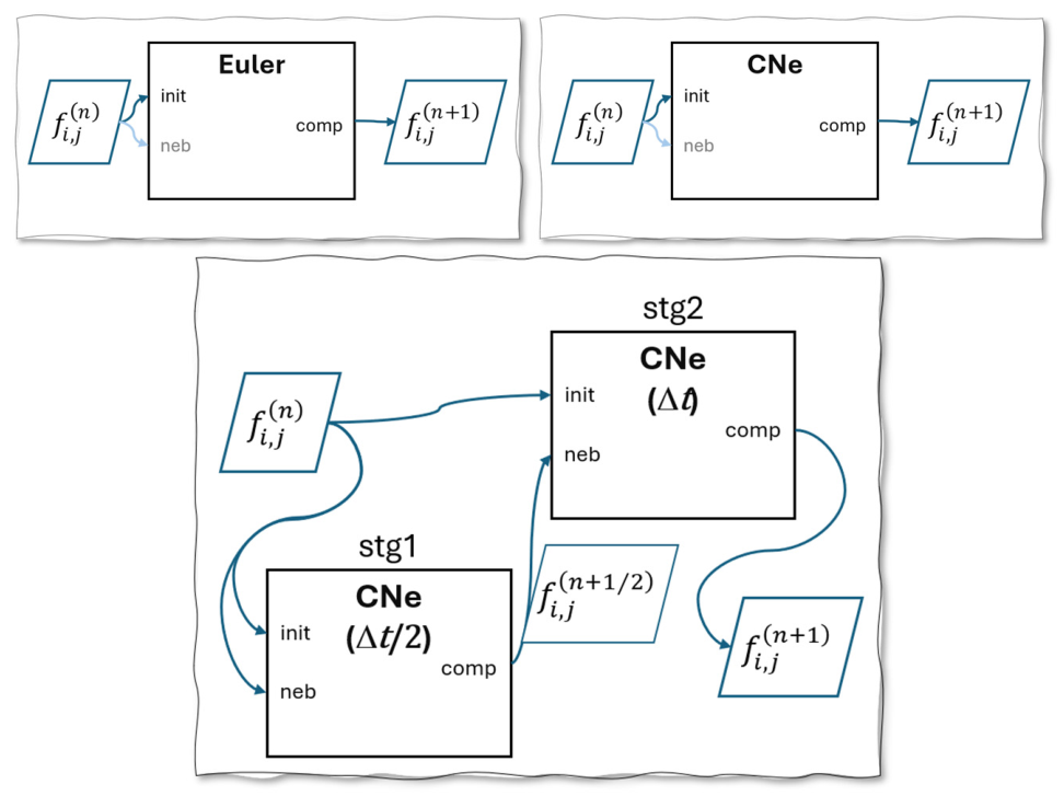
To illustrate the mechanism of the Euler, the CNe, and the CpC methods, see Figure 1.

The CNe and CpC algorithms are unconditionally stable when applied to the diffusion Equation (1); hence, the above mentioned CFL limit does not set any limit to their stability. This excellent stability is implied by the following property.

Theorem 1.

If the CNe or CpC algorithms are used to solve the spatially discretized linear diffusion Equation (1), then, in each timestep, the new $u_{i,j}^n$ values are the convex combinations of the initial values $u_{p,q}^0$.

These statements have been analytically proven in the original papers [21]. Furthermore, the truncation errors of these algorithms for the studied equation are derived in that paper.

2.4. GPU Parallelization and Implementation Strategy

The above methods are well adapted for GPU execution because the value of each inner grid point can be calculated independently within a timestep. A common approach for stencil computations is to assign the calculation of one grid point to one GPU work-item [23]. By doing so, each work-item reads the required values from the previous timestep and writes the new value to its own position in the output grid. Therefore, the work-items do not interfere with each other, and no synchronization is needed during the kernel execution. To interact with the GPU, one has 2 well-known options: OpenCL [24] and CUDA. While CUDA works well with NVIDIA GPU-s, OpenCL has wider compatibility with different platforms [25]. In the present implementation, OpenCL is used to provide a platform-independent GPU programming model [26]. Following this approach, each work-item calculates one inner-domain grid point, while the prescribed boundary values are handled separately. The novelty compared to the previous work [21] is that handling prescribed boundary values is included.

2.4.1. Parallelization of Euler and CNe

In the case of the Euler method, the stepper kernel function for the inner domain is presented in Listing 1. As for the work-item index range this function is parallelly invoked for, the number of indices used to distinguish between work-items equals the number of spatial dimensions. However, only indices denoting the inner domain are used, and the indices of the boundary nodes are omitted. In the 2-dimensional case, supposing a zero-based ({0, …N_x − 1} and {0, …N_y − 1}) indexing, the used index range is {1, …N_x − 2} × {1, …N_y − 2} at each timestep. The host sets no explicit local work-group size, which may lead to implementation-specific behavior of OpenCL.

Listing 1. Kernel of Euler, CNe, and the 1st stage of CpC. This is a verbatim quotation from [21].

#pragma OPENCLEXTENSION cl_khr_fp64: enable   __kernel void calc_cell_2D(                              __global const double *before, __global double *after,                              double2 coeffs, uint2 size, long4 neighbours) {                   const size_t index = get_global_id(0) + size.x * get_global_id(1);                   __global const double *old_cell = before + index;                  after[index] = (1 − 2 * (coeffs.x + coeffs.y)) * *old_cell                              + coeffs.x *                                         (old_cell[neighbours.even.x]                                         + old_cell[neighbours.odd.x])                              + coeffs.y *                                         (old_cell[neighbours.even.y]                                         + old_cell[neighbours.odd.y]); }

where:

• before, after are pointers to the array containing data before and after the timestep;
• coeffs is the [coeff_x, coeff_y] vector containing numerical coefficients for computation;
• size is a vector containing the [N_x, N_y] number of data points; and
• neighbours is a vector containing pointer differences between the current datapoint and its neighbors.

In accordance with (13), the numerical coefficients of the Euler method can be precalculated as:

$$\left[\begin{array}{c}{\mathit{coeff}}_{\mathrm{x}}\\ {\mathit{coeff}}_{\mathrm{y}}\end{array}\right]=D·∆t·\left[\begin{array}{c}{∆x}^{-2}\\ {∆y}^{-2}\end{array}\right]$$

(21)

while—based on (14), (15) and (16)—that of the CNe method can be obtained by:

$$\left[\begin{array}{c}{\mathit{coeff}}_{\mathrm{x}}\\ {\mathit{coeff}}_{\mathrm{y}}\end{array}\right]={\displaystyle \frac{1-\exp \left\{-2D{k}^2∆t\right\}}{2k^2}}·\left[\begin{array}{c}{∆x}^{-2}\\ {∆y}^{-2}\end{array}\right]$$

(22)

where:

k² = ∆x⁻² + ∆y⁻²

(23)

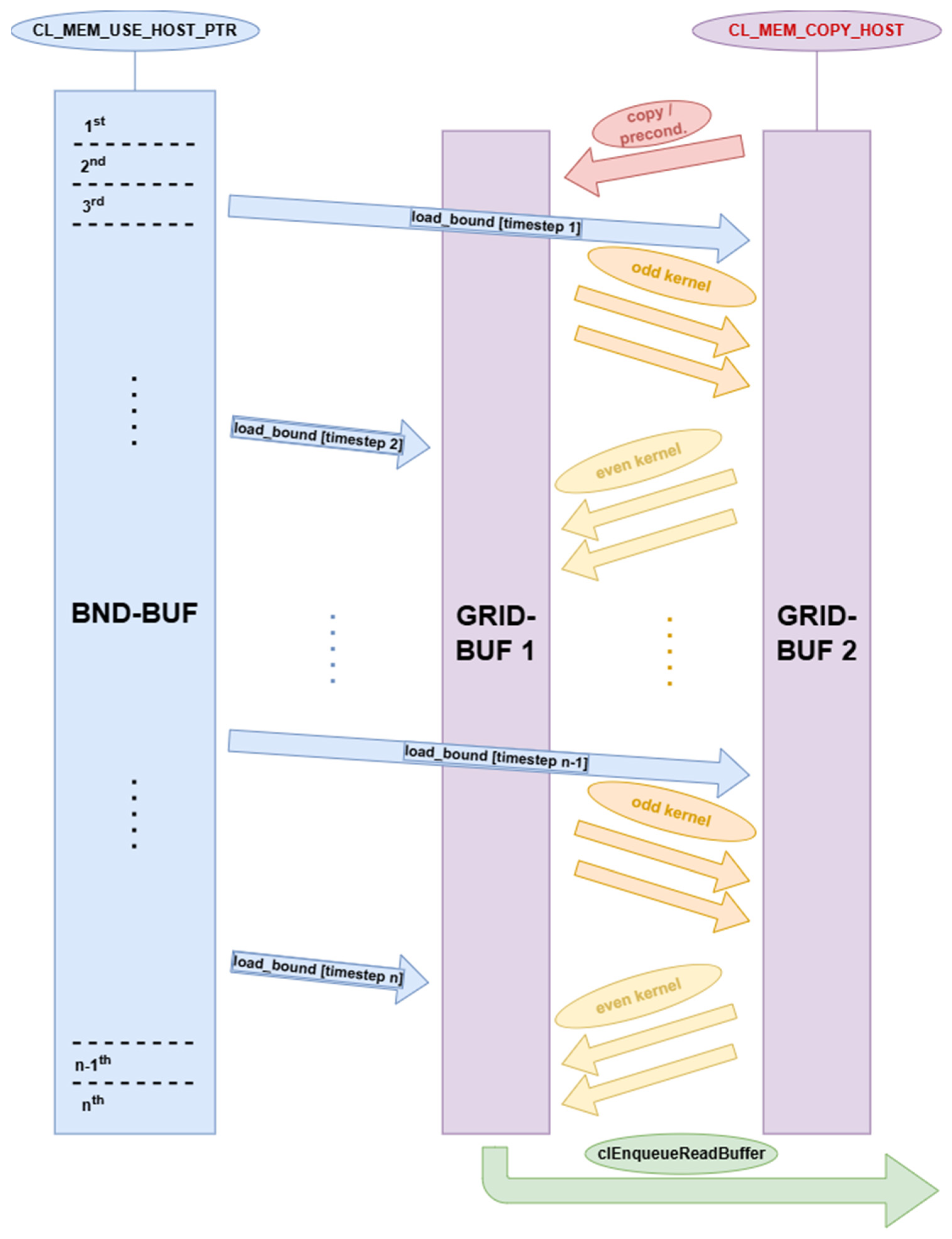
To avoid mixing the values before and after each step, while keeping the memory consumption small, 2 arrays were allocated with enough size to fit the full data-grid in each of them. The roles of the kernel parameters before and after are swapped after each timestep calculation, as shown in Figure 2. At odd timesteps, GRID-BUF 1 is read as values before the step, and GRID-BUF 2 is updated with the result of the timestep calculation. At even timesteps, the roles are swapped. Initial data are placed into GPU RAM by allocating it with the CL_MEM_COPY_HOST flag. Boundary values are accessed by a GPU RAM array allocated with the CL_MEM_USE_HOST_PTR flag and applied to the appropriate buffer by an auxiliary kernel function at each timestep. At the end of the calculation, the result is copied back to the host by a host-side clEnqueueReadBuffer call from the buffer the last timestep calculation has left it in.

The buffer that receives the initial data is allocated using CL_MEM_COPY_HOST_PTR, which means that the data are copied to the GPU RAM at the time of allocation, without any explicit invocation of any further API function. The function clEnqueueCopyBuffer is only used to initially copy the data to the other buffer (this copy is only included to serve as a placeholder for a future preconditioning step.)

The prescribed boundary data are loaded to the grid by a separate kernel function (see Listing 2). The GPU RAM array providing the boundary data is allocated using CL_MEM_USE_HOST_PTR, allowing the OpenCL implementation to use the supplied host-memory region without fully copying the data at allocation time. The exact realization of host-device data movement is implementation-dependent and is handled by the OpenCL runtime.

Listing 2. Kernel to apply boundary data.

#pragma OPENCLEXTENSION cl_khr_fp64: enable __kernel void load_bound(                              __global double *datagrid, __global const double *bound_evol,                              const uint tm_offs, const unsigned long *idx_tbl, uint bndsize) {                   __global const double *timeframe = bound_evol + tm_offs;                   const size_t i = get_global_id(0);                   datagrid[idx_tbl[i]] = timeframe[i]; }

where:

• datagrid are pointers to the datagrid the boundary data is being loaded into;
• bound_evol is a pointer to the array containing the boundary evolution data;
• tm_offs is the time-proportional offset inside array bound_evol;
• idx_tbl is an index-table containing the offset values of the boundary data-points inside datagrid; and
• bndsize is the size of the boundary values per timestep (same as the total number of work-items).

In the 1D case, the index-table simply contains the offset value of the left and right endpoints. In 2D, the table contains the following offset values:

• Offset values of the 4 corner nodes;
• The N_x − 2 offset values of the j = 1 vertex;
• The N_y − 2 offset values of the i = N_x vertex;
• The N_x − 2 offset values of the j = N_y vertex;
• The N_y − 2 offset values of the i = 1 vertex.

For this kernel, only one level of work-item indexing is used. The size of the index-table, as well as the index-range of the kernel, is {0, …2·(N_x + N_y) − 4}.

To summarize, the steps the solver must execute are the following:

• Load initial and boundary data from file to host RAM;
• Initialize OpenCL and build kernel code;
• Allocate GPU memory for 2 full data-grids, containing a copy of the initial data, and one more GPU RAM array for boundary data (with “using HOST pointer” mode);
• Acquire kernel instances and parametrize them for the time evolution loop;
• Enqueue execution of boundary loader kernel;
• Enqueue execution of inner-domain kernel function. Roles of the 2 full-grid memory buffers depend on the parity of the current timestep;
• Swap the roles of the 2 full-grid memory buffers to prepare for next timestep iteration;
• Go back to 5 and repeat the loop until the last timestep is handled;
• Enqueue reading back the result from the last written full-grid GPU buffer to RAM;
• Wait until all data movements are finished;
• Release kernel resources and GPU RAM;
• Write results to file;
• On exit, release any remaining OpenCL resources.

It is to be remarked at about step 3 that only one of the 2 grid buffers is allocated containing the initial data (using the CL_MEM_COPY_HOST flag). The data are copied to the other buffer between steps 4 and 5 by a host-side clEnqueueCopyBuffer call. This intermediate step is a placeholder for a possible preprocessing step of a future version.

2.4.2. Parallelization of CpC

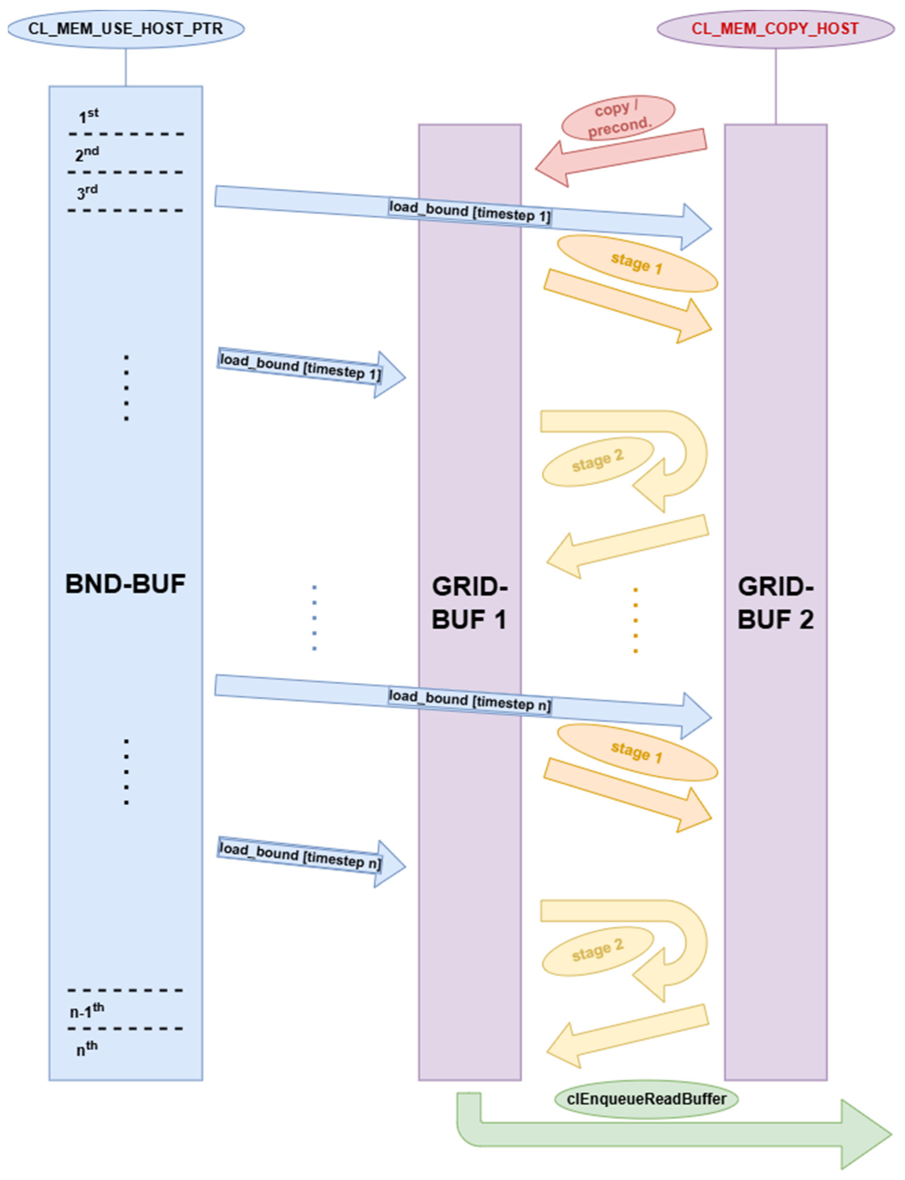
In the case of CpC, two ranges of kernels need to be executed at each timestep. Again, two arrays need to be allocated, but—as shown in Figure 3—their roles are never swapped: one array is to store the full-step values, and the other is to store the midpoint predictions. The calculation of each timestep consists of 2 stages, having different kernel functions. The first stage reads the values from GRID-BUF 1 and stores its result in GRID-BUF 2. The second stage calculates the neighboring effect from the values stored in GRID-BUF 2 and updates values in GRID-BUF 1 based on it. Initial data are placed into GPU RAM by allocating it with the CL_MEM_COPY_HOST flag. Boundary values are accessed by a GPU RAM array (BND_BUF) allocated with the CL_MEM_USE_HOST_PTR flag and applied to GRID-BUF 1 and GRID-BUF 2 by an auxiliary kernel at each timestep. At the end of the calculation, the result is copied from buffer 1 back to the host by a host-side clEnqueueReadBuffer call.

The first stage can use the same kernel function as in the case of Euler and CNe, but—according to (19)—compared to CNe, the factor of 2 is missing from the exponent:

$$\left[\begin{array}{c}{\mathit{coeff}}_{\mathrm{x}}\\ {\mathit{coeff}}_{\mathrm{y}}\end{array}\right]={\displaystyle \frac{1-\exp \left\{-D{k}^2∆t\right\}}{2k^2}}·\left[\begin{array}{c}{∆x}^{-2}\\ {∆y}^{-2}\end{array}\right]$$

(24)

The second-stage kernel needs to be slightly modified because it needs to obtain the pre-stage values and the neighboring effect from 2 different arrays, as shown in Listing 3.

Listing 3. Kernel of the 2nd stage of CpC. This is a verbatim quotation from [21].

__kernel void stage2p05_calc_cell_2D(                             __global const double *stage0,                             __global const double *stage1,                             __global double *after,                             double2 coeffs, uint2 size, long4 neighbours) {                   const size_t index = get_global_id(0) + size.x * get_global_id(1);                   __global const double *old_cell = stage0 + index;                   __global const double *midpoint = stage1 + index;                   after[index] = (1 − 2 * (coeffs.x + coeffs.y)) * *old_cell                             + coeffs.x *                                        (midpoint[neighbours.even.x] +                                        midpoint[neighbours.odd.x])                             + coeffs.y *                                        (midpoint[neighbours.even.y] +                                        midpoint[neighbours.odd.y]); }

where:

• stage0 is a pointer to the array containing data before stage 1;
• stage1 is a pointer to the array containing the result of stage 1;
• after is a pointer to the array containing data after all the stages (often the same as stage0);
• coeffs is the [coeff_x, coeff_y] vector containing numerical coefficients for computation;
• size is a vector containing the [N_x, N_y] number of data points; and
• neighbours is a vector containing pointer differences between the current datapoint and its neighbours.

For parameter stage0 and after, the same array is specified, allowing the function to update the values in-place. Based on (20), the coefficients are calculated again by (22).

To summarize, the steps the solver must execute are the following:

• Load initial and boundary data from file to CPU RAM;
• Initialize OpenCL and build kernel code;
• Allocate GPU memory for 2 full datagrids, containing a copy of the initial data, and one more GPU RAM array for boundary data (with “using HOST pointer” mode).
• Acquire kernel instances and parametrize them for the time evolution loop;
• Enqueue execution of boundary loader kernel for the mid-point buffer;
• Enqueue execution of stage 1 inner-domain kernel function;
• Enqueue execution of boundary loader kernel for the full-step buffer;
• Enqueue execution of stage 2 inner-domain kernel function;
• Go back to 5 and repeat the loop until the last timestep is handled;
• Enqueue reading back result from full-step GPU buffer to RAM;
• Wait until all data movements are finished;
• Release kernel resources and GPU RAM;
• Write results to file;
• On exit, release any remaining OpenCL resources.

3. General Information About the Way of Investigation

This section introduces the applied numerical problem and shortly presents the principles of the comprehensive studies (see Section 3.1) performed on the algorithms listed in Section 2.3, presents the mathematical case studies used as test cases (Section 3.2), and sets up the general circumstances of the investigations by introducing some basic definitions (Section 3.3) related to the examination methodology and listing the technical data of the applied computer (Section 3.4).

3.1. The Types of Examinations Being Performed

If one has an analytical solution with an infinite spatial domain of the equation, Dirichlet’s variable boundary condition can be used to simulate the solution on a finite domain. To achieve this, one has to sample the time evolution of the analytical solution on the boundaries of the simulation domain and prepare it for the algorithm as predefined boundary values. This approach is used in this work for a non-trivial analytical solution of the heat equation, presented in detail in Section 3.2.1 and Section 3.2.2. At the end of the day, three types of examinations have been performed (each of Section 4, Section 5 and Section 6 presents one of these examinations):

• General benchmarking of the three methods: The algorithmic error is shown as a function of the computation time, as well as that of the timestep size. Curves belonging to different algorithms are plotted on the same figure. The execution time is examined as a function of the total number of spatial grid points. This allows seeing the trade-off between computations with different numbers of spatial dimensions;
• Examining the depletion of GPU, as the system-size is being enlarged: The computation time is plotted both as a function of the total number of spatial grid-points and—for the CpC method—as a function of the timestep count;
• Examining the error convergence of the CpC method when refining the timescale: The algorithmic error is examined as a function of the timestep size. The error should converge to a small residual value, as the timestep size is decreased. Curves for multiple grids are presented on the same figure.

3.2. Initial Value Problems

3.2.1. One-Dimensional Initial Value Problems

In one-dimensional computations, the following analytical solution of (1) was used as a mathematical case study:

$$U\left(x,t\right)=A_0·\exp \left\{-{\displaystyle \frac{x^2}{4\mathit{Dt}}}\right\}·\left(1-{\displaystyle \frac{x^2}{2\mathit{Dt}}}+{\displaystyle \frac{x^4}{20D^2{t}^2}}-{\displaystyle \frac{x^6}{840D^3{t}^3}}\right)·{\displaystyle \frac{x}{t^{9/2}}}$$

(25)

where:

• $A_0=1/\underset{x}{\max }\left|{\left.U\left(x,t=T_{\mathrm{init}}\right)\right|}_{A_0=1}\right|$ is the norming factor, and
• D = 1 is the diffusion coefficient.

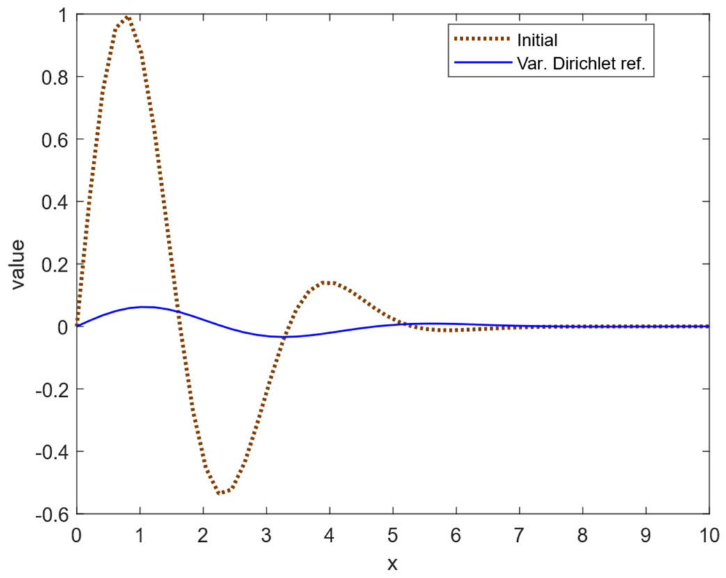
As an example, for T_init = 1 and T_fin = 2 (the values used with the CNe and CpC method), the initial function and the reference solution are shown in Figure 4.

3.2.2. Two-Dimensional Initial Value Problem

In two dimensions, the direct product of (25) is taken with itself, and the result is renormalized:

$$U\left(x,y,t\right)=A_0·\exp \left\{-{\displaystyle \frac{x^2+y^2}{4\mathit{Dt}}}\right\}·$$

$$\left(1-{\displaystyle \frac{x^2}{2\mathit{Dt}}}+{\displaystyle \frac{x^4}{20D^2{t}^2}}-{\displaystyle \frac{x^6}{840D^3{t}^3}}\right)$$

$$\left(1-{\displaystyle \frac{y^2}{2\mathit{Dt}}}+{\displaystyle \frac{y^4}{20D^2{t}^2}}-{\displaystyle \frac{y^6}{840D^3{t}^3}}\right)·{\displaystyle \frac{\mathit{xy}}{t^9}}$$

(26)

where:

• $A_0=1/\underset{x,y}{\max }\left|{\left.U\left(x,y,t=T_{\mathrm{init}}\right)\right|}_{A_0=1}\right|$ is the new norming factor, and
• D = 1 is the diffusion coefficient.

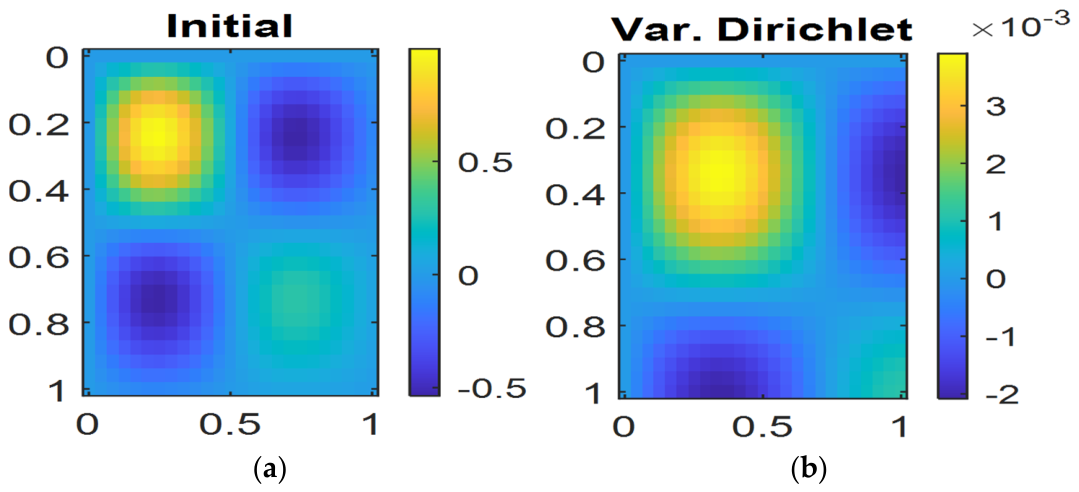
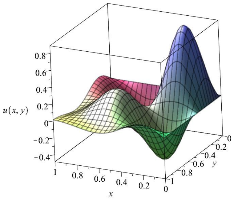
An illustration of the analytical solution can be seen in Figure 5 and Figure 6.

3.3. Measuring Execution Time, Definition of Algorithmic Error

In the recent work, the examined algorithm is invoked four times for each test case, and an average execution time value is calculated with deviations:

$$t_{\mathrm{exec}}\left(N_{\mathrm{r}},N_{\mathrm{t}}\right)={\displaystyle \frac{1}{R}}{\sum }_{r=1}^R{t}_{\mathrm{exec}}^{\left(r\right)}\left(N_{\mathrm{r}},N_{\mathrm{t}}\right),$$

(27)

where $t_{\mathrm{exec}}^{\left(r\right)}\left(N_{\mathrm{r}},N_{\mathrm{t}}\right)$ is the execution time of the r-th experiment with N_r spatial nodes and N_t timestep size. A repetition number of R = 4 is used, except in Section 5, where experiments based on the parameters described in Section 5.1.2 are repeated only 3 times to save some time.

The error of the algorithms is defined as the L_∞ distance between the computation output of the final timestep and the reference (the analytical) solution:

$${\mathit{err}}^{\max }=\underset{i,j}{\max }\left|u_{i,j}^{N_{\mathrm{t}},\mathrm{comp}}-u_{i,j}^{\mathrm{anal}}\right|,$$

(28)

which can be considered as a function of the ∆t timestep size.

3.4. The Technical Specifications of the Computer Being Used

The applied computer has the following specifications:

• CPU: Gen11 Intel Core i7-11700F, 2.5 GHz;
• RAM: 64 GB;
• OS: Windows 11 Enterprise (24H2), ×64;
• GPU: NVIDIA, 12GB;
• OpenCL: Intel v2020.3.494;
• MATLAB: R2025B.

4. General Benchmarking of the Three Methods

In this examination, all the three methods are included, and they are benchmarked by making two types of plots:

• The first type of plot shows algorithmic error as a function of the execution time. For benchmarking reasons, data of different algorithms are plotted as different curves on the same figure. For different numbers of spatial dimensions, different figures are created;
• The second type of plot shows the algorithmic error as a function of the timestep size, to enable parameter-wise benchmarking.

The scaling parameters of the investigation, the resulting plots, and the discussion can be found in the subsequent subsections (Section 4.1, Section 4.2 and Section 4.3, respectively).

4.1. Scaling Parameters

The timescale and spatial grid parameters used for the one-dimensional computations are shown in

Table 1. Timescale parameters used with 1-dimensional computations.

Nt	Δt	Nt	Δt
9	1.111 × 10−1	15,000	6.667 × 10−5
15	6.667 × 10−2	30,000	3.333 × 10−5
30	3.333 × 10−2	50,000	2.000 × 10−5
50	2.000 × 10−2	90,000	1.111 × 10−5
150	6.667 × 10−3	150,000	6.667 × 10−6
300	3.333 × 10−3	300,000	3.333 × 10−6
500	2.000 × 10−3	500,000	2.000 × 10−6
900	1.111 × 10−3	900,000	1.111 × 10−6
1500	6.667 × 10−4	1,500,000	6.667 × 10−7
3000	3.333 × 10−4	3,000,000	3.333 × 10−7
5000	2.000 × 10−4	5,000,000	2.000 × 10−7
9000	1.111 × 10−4	9,000,000	1.111 × 10−7

The simulated time interval is always [T_init, T_fin] = [1, 2].

and

Table 2. Parameters of 1-dimensional spatial grids.

Nx	Δx
100	1.010 × 10−1
1000	1.001 × 10−2

The simulated spatial interval is always [X_init, X_fin] = [0, 10].

, respectively.

The timescale and spatial grid data used for the two-dimensional computations are in

Table 3. Timescale parameters used with 2-dimensional computations.

Nt	Δt	Nt	Δt
9	1.111 × 10−2	5000	2.000 × 10−5
15	6.667 × 10−3	9000	1.111 × 10−5
30	3.333 × 10−3	15,000	6.667 × 10−6
50	2.000 × 10−3	30,000	3.333 × 10−6
150	6.667 × 10−4	50,000	2.000 × 10−6
300	3.333 × 10−4	90,000	1.111 × 10−6
500	2.000 × 10−4	150,000	6.667 × 10−7
900	1.111 × 10−4	300,000	3.333 × 10−7
1500	6.667 × 10−5	600,000	1.667 × 10−7
3000	3.333 × 10−5	900,000	1.111 × 10−7

The simulated time interval is always [T_init, T_fin] = [0.1, 0.2].

and

Table 4. Parameters of 2-dimensional spatial grids.

Nx	Ny	Nx * Ny	Δx⋅Δy
40	40	1600	6.575 × 10−4
100	100	10,000	1.020 × 10−4

The simulated spatial interval is always [X_init, X_fin] = [0, 1] and [Y_init, Y_fin] = [0, 1].

.

4.2. Results

The results of the one-dimensional and two-dimensional computations are listed in separate subsections (Section 4.2.1 and Section 4.2.2, respectively).

4.2.1. Error—Computation Time Characteristics, One-Dimensional Computation

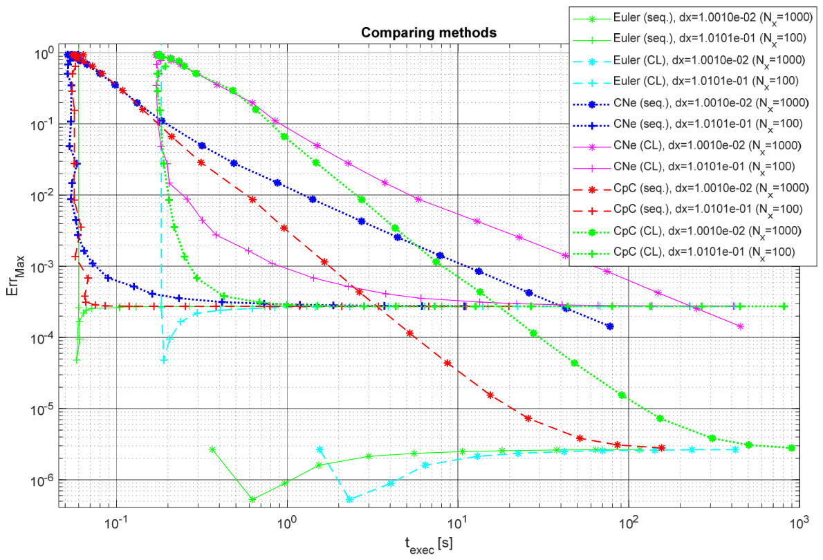
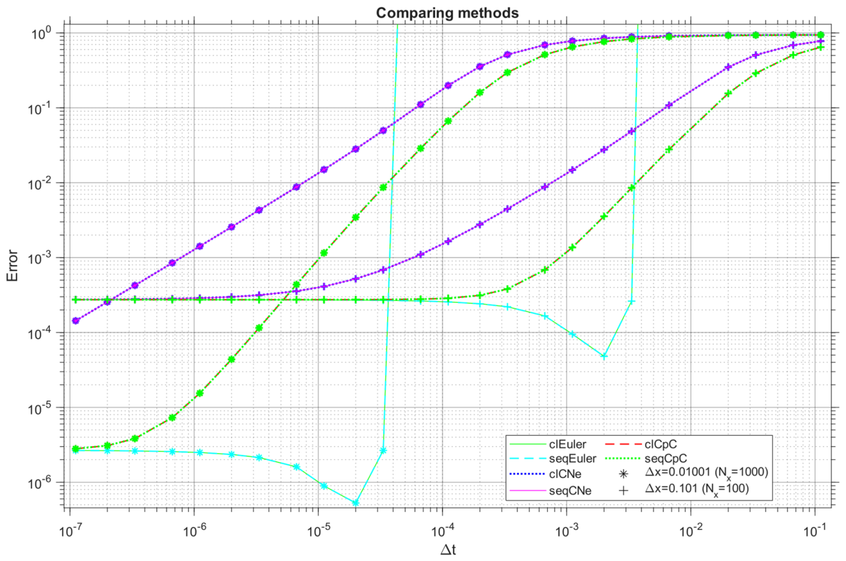
The measurement results (i.e., the algorithmic error, as a function of the execution time) of the one-dimensional computations can be seen in Figure 7. For clearer comparability, the data are also plotted as a function of the timestep size in Figure 8.

4.2.2. Error—Computation Time Characteristics, Two-Dimensional Computation

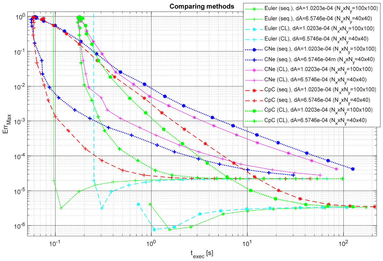
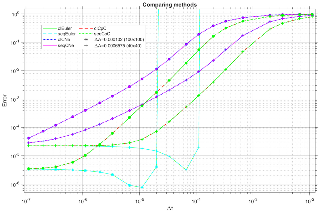
The results of the two-dimensional experiments are presented in Figure 9. Figure 10 shows data as a function of the timestep size.

4.3. Discussion

In Figure 7, Figure 8, Figure 9 and Figure 10, the stability problems of the Euler method are observable, while it can also be seen that in the stable region, the Euler method is more accurate than the rest of the methods. In Figure 8, grid-related information can be read: For the N_x = 100 grid (∆x = 1.010 × 10⁻¹) Euler method becomes unstable at ∆t > 3.333 × 10⁻³ (N_t < 300), while for N_x = 1000 (∆x = 1.001 × 10⁻²), the instability comes at ∆t > 3.333 × 10⁻⁵ (N_t < 30,000). In Figure 10, further grid-related information can be seen, showing that for N_x × N_Y = 100 × 100 (∆x∆y = 1.020 × 10⁻⁴), the instability arrives at ∆t > 1.111 × 10⁻⁴ (N_t < 900), while for N_x × N_Y = 40 × 40 (∆x∆y = 6.575 × 10⁻⁴), stability holds only until ∆t > 2.0 × 10⁻⁵ (N_t < 5000). In Figure 8 and Figure 10, the curves of the sequential and the OpenCL-based version of the same algorithm are identical, verifying that parallelization produces the same numerical result as the sequential implementation. All these experiences are in accordance with the previous paper of the authors.

5. Acceleration and Depletion of Parallel Computation Capacity for Increasing System Size

In our previous work [21], the execution time of the algorithms proved to be almost independent of the number of spatial nodes; hence, we decided to further investigate the dependency of computation time both on the spatial node count and the timestep count. This examination consists of 2 parts:

• The data acquisitions of Section 4 are repeated with a grid-sweep up to a much higher—40,000 by 40,000—node count. Computation time is plotted as a function of the total number of spatial nodes;
• In the case of the CpC method, the above experiment is repeated with two more timescales, and another set of timescales and grids (with a much lower node count) are introduced to gain insight into the dependency on both the node count and the timestep count. As no accurate fitting model was found by the authors to explain the results, two types of figures were plotted to analyze performance on huge systems:

  ○

  one to show the effect of timestep count, and

  ○

  one to show the dependence on the spatial resolution.

Since these examinations can involve spatial grids with high node counts, the calculation of algorithmic error is omitted to save memory space, and only computation time is compared. (i.e., the tester code is configured to refuse reference calculation and to release memory of initial data after it is saved to a file and passed to the target algorithm.)

The subsequent subsections contain the scaling information, the resulting plots, and the discussion (Section 5.1, Section 5.2 and Section 5.3, respectively).

5.1. Scaling Parameters

The cross-method benchmarking and the performance analysis of CpC use different spatial and temporal scaling, which are presented in Section 5.1.1 and Section 5.1.2.

5.1.1. Comparing All the Methods on Big Systems

The timescale and spatial grid parameters of the one-dimensional computations are contained in

Table 5. Timescale parameters used with 1-dimensional computations to examine depletion of GPU.

Tinit	Tfin	Nt	Δt
1	2	500	2.000 × 10−3

and

Table 6. Parameters of 2-dimensional spatial grids used to examine depletion of GPU.

Nx	Δx	Nx	Δx
40	2.564 × 10−1	4,000,000	2500 × 10−6
120	8.403 × 10−2	* 5,000,000	2000 × 10−6
400	2.506 × 10−2	* 7,000,000	1429 × 10−6
1200	8.340 × 10−3	* 9,000,000	1111 × 10−6
4000	2.501 × 10−3	12,000,000	8333 × 10−7
12,000	8334 × 10−4	* 16,000,000	6250 × 10−7
40,000	2.500 × 10−4	* 22,000,000	4545 × 10−7
* 50,000	2.000 × 10−4	* 30,000,000	3333 × 10−7
* 70,000	1.429 × 10−4	40,000,000	2500 × 10−7
* 90,000	1.111 × 10−4	* 50,000,000	2000 × 10−7
120,000	8.333 × 10−5	* 70,000,000	1429 × 10−7
* 160,000	6.250 × 10−5	* 90,000,000	1111 × 10−7
* 220,000	4.545 × 10−5	120,000,000	8333 × 10−8
* 300,000	3.333 × 10−5	* 160,000,000	6250 × 10−8
400,000	2.500 × 10−5	* 220,000,000	4545 × 10−8
* 500,000	2.000 × 10−5	* 300,000,000	3333 × 10−8
* 700,000	1.429 × 10−5	400,000,000	2500 × 10−8
* 900,000	1.111 × 10−5	* 500,000,000	2000 × 10−8
1,200,000	8.333 × 10−6	* 700,000,000	1429 × 10−8
* 1,600,000	6.250 × 10−6	* 900,000,000	1111 × 10−8
* 2,200,000	4.545 × 10−6	1,200,000,000	8333 × 10−9
* 3,000,000	3.333 × 10−6

The simulated spatial interval is always [X_init, X_fin] = [0, 10], * Marked records are only used in the OpenCL case.

, while those of the two-dimensional computations are shown in

Table 7. Timescale parameters used with 2-dimensional computations to examine depletion of GPU.

Tinit	Tfin	Nt	Δt
0.1	0.2	500	2.000 × 10−4

and

Table 8. Parameters of 2-dimensional spatial grids used to examine depletion of GPU.

Nx	Ny	Nx * Ny	Δx * Δy	Nx	Ny	Nx * Ny	Δx * Δy
65	65	4225	2.441 × 10−4	* 2830	2830	8,008,900	1.249 × 10−7
100	100	10,000	1.020 × 10−4	* 3360	3360	11,289,600	8.863 × 10−8
200	200	40,000	2.525 × 10−5	4000	4000	16,000,000	6.253 × 10−8
* 238	238	56,644	1.780 × 10−5	* 4520	4520	20,430,400	4.897 × 10−8
* 283	283	80,089	1.257 × 10−5	* 5100	5100	26,010,000	3.846 × 10−8
* 336	336	112,896	8.911 × 10−6	* 5760	5760	33,177,600	3.015 × 10−8
400	400	160,000	6.281 × 10−6	6500	6500	42,250,000	2.368 × 10−8
* 452	452	204,304	4.916 × 10−6	* 7240	7240	52,417,600	1.908 × 10−8
* 510	510	260,100	3.860 × 10−6	* 8060	8060	64,963,600	1.540 × 10−8
* 576	576	331,776	3.025 × 10−6	* 8980	8980	80,640,400	1.240 × 10−8
650	650	422,500	2.374 × 10−6	10,000	10,000	100,000,000	1.000 × 10−8
* 724	724	524,176	1.913 × 10−6	* 11,900	11,900	142,000,000	7.074 × 10−9
* 806	806	649,636	1.543 × 10−6	* 14,100	14,100	199,000,000	5.037 × 10−9
* 898	898	806,404	1.243 × 10−6	* 16,800	16,800	282,000,000	3.547 × 10−9
1000	1000	1,000,000	1.002 × 10−6	20,000	20,000	400,000,000	2.503 × 10−9
* 1190	1190	1,416,100	7.074 × 10−7	* 23,800	23,800	566,440,000	1.767 × 10−9
* 1410	1410	1,988,100	5.037 × 10−7	* 28,300	28,300	800,890,000	1.249 × 10−9
* 1680	1680	2,822,400	3.547 × 10−7	* 33,600	33,600	112,896,000	8.858 × 10−10
2000	2000	4,000,000	2.503 × 10−7	40,000	40,000	1,600,000,000	6.250 × 10−10
* 2380	2380	5,664,400	1.767 × 10−7

The simulated spatial interval is always [X_init, X_fin] = [0, 1] and [Y_init, Y_fin] = [0, 1], * Marked records are only used in the OpenCL case.

, respectively.

5.1.2. Analyzing Performance of CpC Method

The scaling data of the benchmarking is readable in

Table 9. Timescale parameters used with 1-dimensional computations to examine depletion of GPU.

Nt	Δt	Nt	Δt
1	1.000 × 100	5000	2.000 × 10−4
5	2.000 × 10−1	50,000	2.000 × 10−5
50	2.000 × 10−2	* 200,000	5.000 × 10−6
500	2.000 × 10−3

The simulated time interval is always [T_init, T_fin] = [1, 2], * Omitting the two greatest spatial grid-point counts in both sequential and OpenCL cases.

,

Table 10. Parameters of 1-dimensional spatial grids used to examine depletion of GPU.

Nx	Δx	Nx	Δx
40	2564 × 10−1	120,000	8333 × 10−5
120	8403 × 10−2	400,000	2500 × 10−5
400	2506 × 10−2	* 1,200,000	8333 × 10−6
1200	8340 × 10−3	* 4,000,000	2500 × 10−6
4000	2501 × 10−3	** 12,000,000	8333 × 10−7
12,000	8334 × 10−4	** 40,000,000	2500 × 10−7
40,000	2500 × 10−4

The simulated spatial interval is always [X_init, X_fin] = [0, 10], * For N_t = 200,000, marked records are only used in the OpenCL case. ** Marked records are only used in the OpenCL case.

,

Table 11. Timescale parameters used with 1-dimensional computations to examine depletion of GPU.

Nt	Δt	Nt	Δt
1	1.000 × 10−1	5000	2.000 × 10−5
5	2.000 × 10−2	50,000	2.000 × 10−6
50	2.000 × 10−3	* 200,000	5.000 × 10−7
500	2.000 × 10−4

Simulated time interval is always [T_init, T_fin] = [0.1, 0.2], * Omitting the two greatest spatial grid-point counts in both sequential and OpenCL cases.

and

Table 12. Parameters of 2-dimensional spatial grids used to examine depletion of GPU

Nx	Ny	Nx * Ny	Δx * Δy	Nx	Ny	Nx * Ny	Δx * Δy
65	65	4225	2441 × 10−4	* 1000	1000	1,000,000	1002 × 10−6
100	100	10,000	1020 × 10−4	* 2000	2000	4,000,000	2503 × 10−7
200	200	40,000	2525 × 10−5	** 4000	4000	16,000,000	6253 × 10−8
400	400	160,000	6281 × 10−6	** 6500	6500	42,250,000	2368 × 10−8
650	650	422,500	2374 × 10−6

The simulated spatial interval is always [X_init, X_fin] = [0, 1] and [Y_init, Y_fin] = [0, 1], * For N_t = 200,000, marked records are only used in the OpenCL case. ** Marked records are only used in the OpenCL case.

. In the case of these experiments, a repetition count of R = 3 is used.

5.2. Results

The results of the analysis of CpC with respect to timestep count dependence, the results of the analysis with respect to spatial node count dependence, and the results of the cross-method benchmarking are presented in different subsections (Section 5.2.1, Section 5.2.2 and Section 5.2.3, respectively).

5.2.1. Computation Time of CpC, Depending on Timestep Count

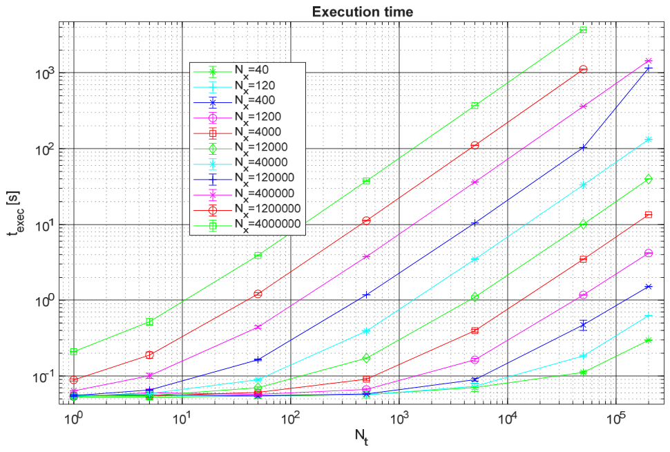
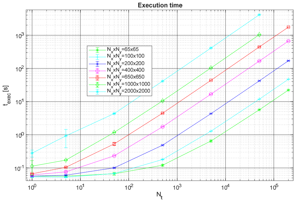
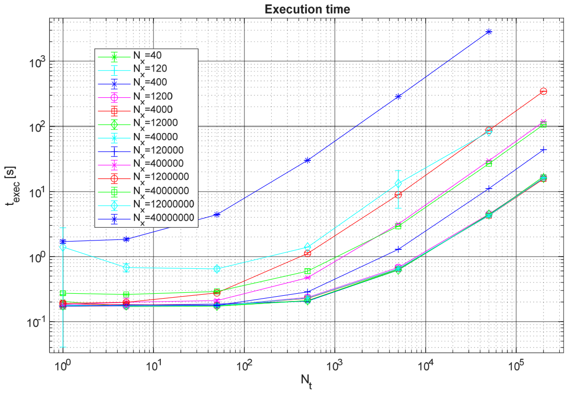
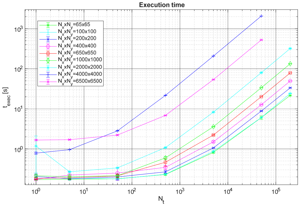
As for the detailed examination of the CpC, the computation time of the one-dimensional computations, as a function of the timestep count, can be seen in Figure 11 for sequential and Figure 12 for parallelized versions. The same graphs for two-dimensional computations are presented in Figure 13 and Figure 14, respectively.

5.2.2. Computation Time of CpC, Depending on Spatial Node Count, Seeing Depletion of GPU

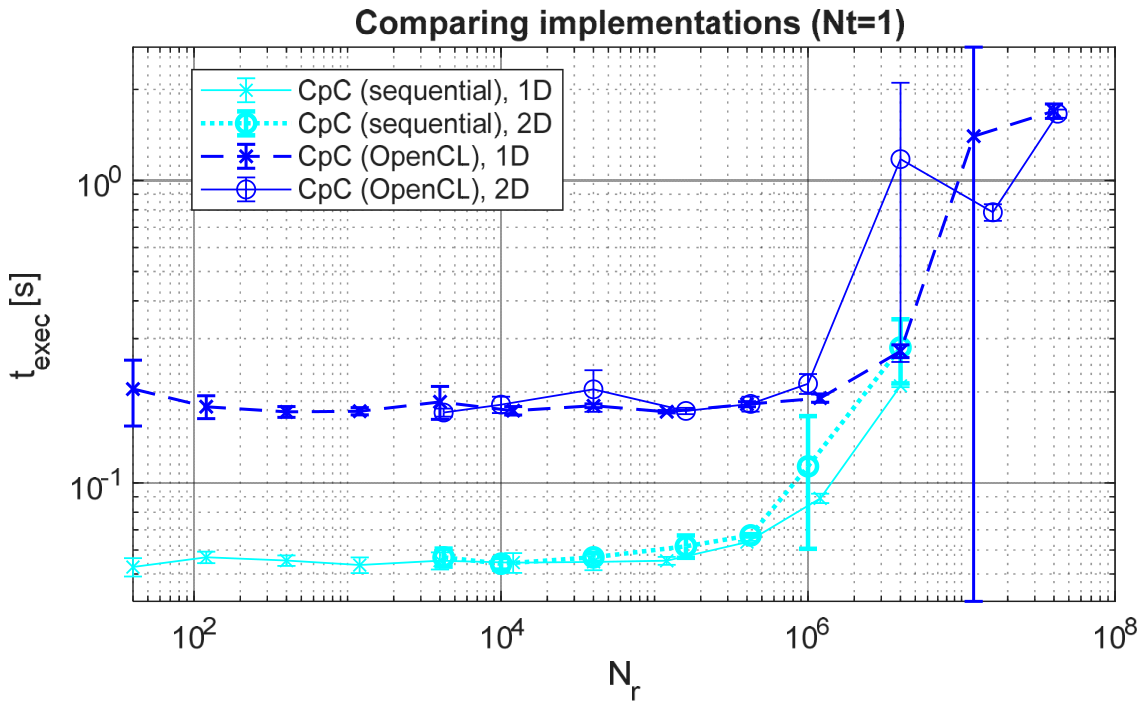
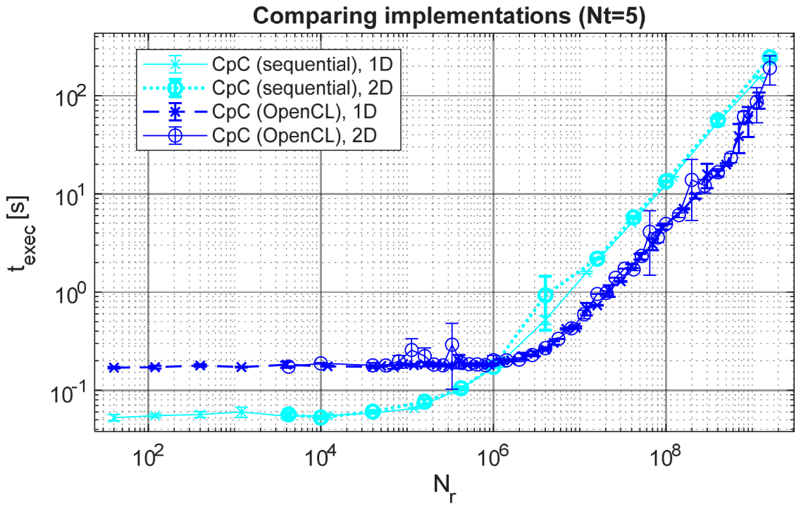
The cross-dimensional, cross-implementation benchmarking graphs can be seen in Figure 15, Figure 16, Figure 17, Figure 18, Figure 19, Figure 20 and Figure 21. Each figure shows performance for different timestep counts.

5.2.3. Comparing Different Algorithms, Seeing Depletion of GPU

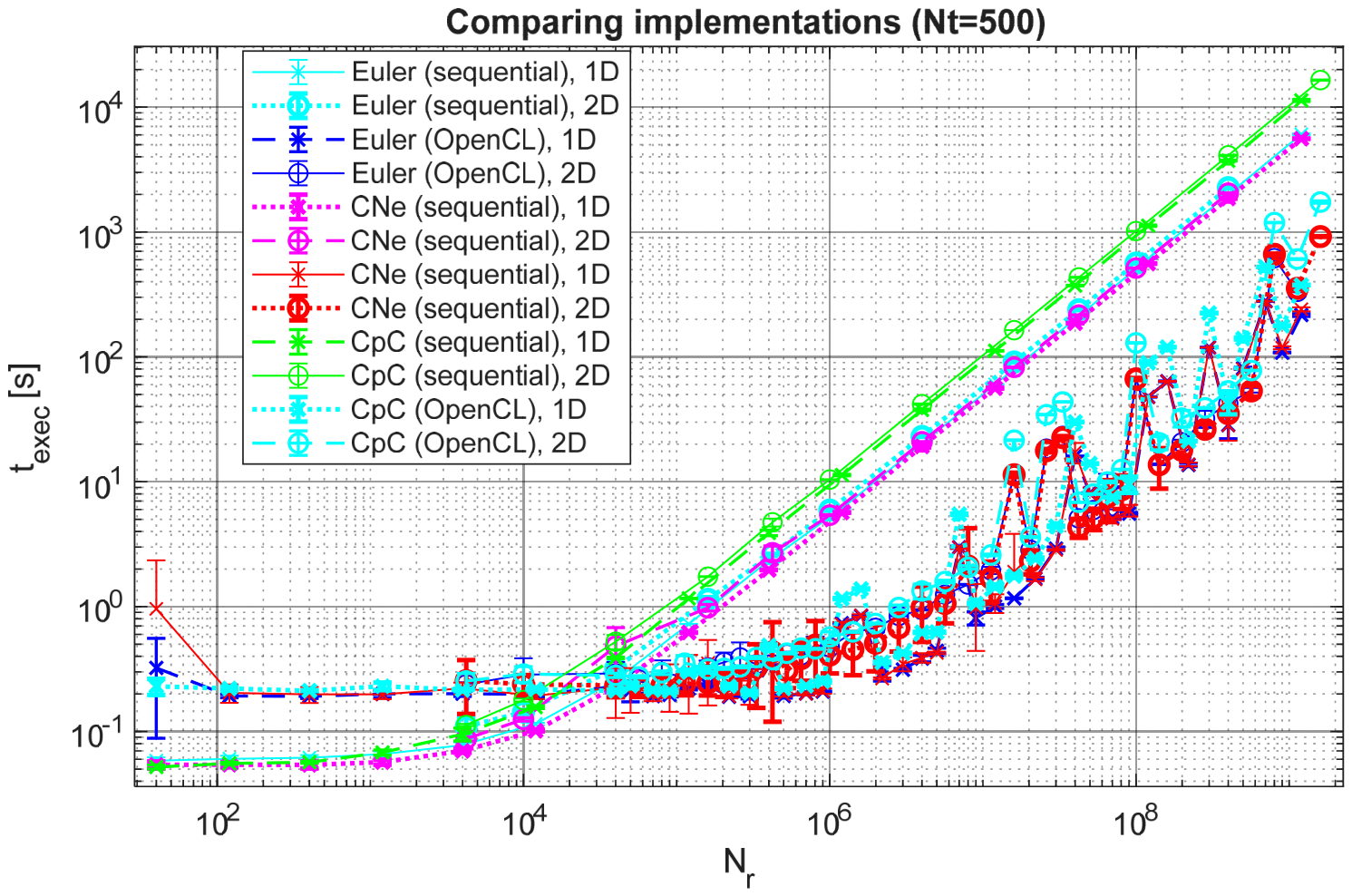
The 500-timestep case of Section 5.2.2 (Figure 18) is repeated, showing the performance of other algorithms in Figure 22.

5.3. Discussion

In our previous work, the computation time of the OpenCL-based versions seemed to be independent of the number of spatial grid-points (only in the case of two-dimensional computations, a slight increase could be observed over 20–30 thousand spatial node count) [21]. The probable reason was that the parallel computation capacity of the GPU was not depleted; hence, adding any further task did not increase the necessary computation time significantly.

In Section 5.2.1 (Figure 11, Figure 12, Figure 13 and Figure 14), it can be observed that each computation has some time-cost independently from the number of timesteps, supposedly related to reading the initial data and other administrative costs. In the case of parallelized implementation—where the application needs to allocate GPU resources and forward the initial data into it—this initial time cost is slightly greater, and sometimes temporarily decreases to have a minimum at around N_t = 5.

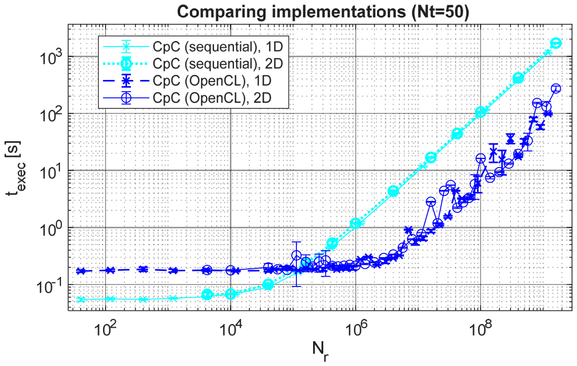
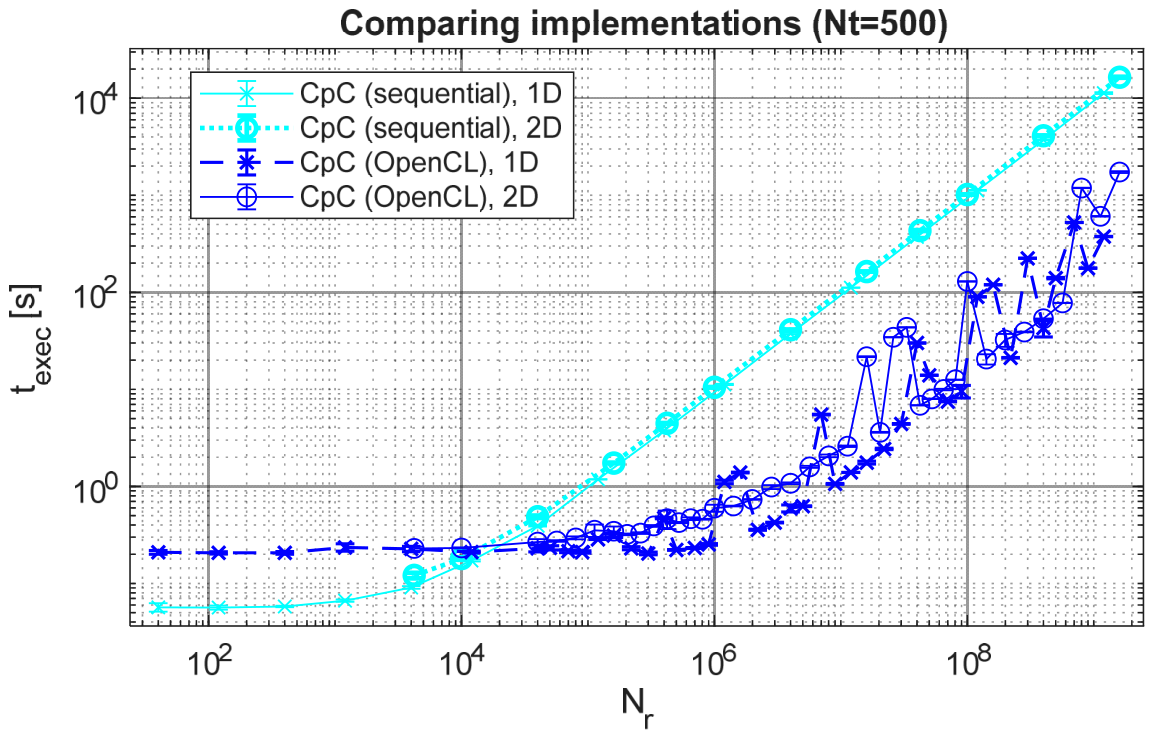
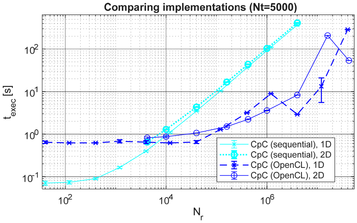
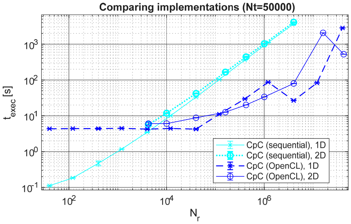
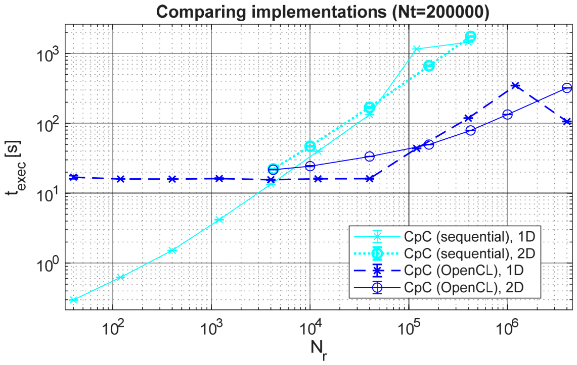
In Section 5.2.2 (Figure 15, Figure 16, Figure 17, Figure 18, Figure 19, Figure 20 and Figure 21), examining the dependence on the number of spatial nodes, the crossover point where parallelization becomes advantageous decreases as the timestep count is increased. Because of the initial cost observable in Section 5.2.1, performing a single timestep, OpenCL proves to be slower until the end of the curve (see Figure 15), which is at N_r = 4 × 10⁶. For N_t = 5, the crossover point is lowered to N_r = 10⁶, and for N_t = 500, it has decreased to N_r = 2 × 10⁴. Then, the decrease becomes slower; it is around N_r = 5000 for N_t = 50,000 (the case examined in the previous work of the authors), and around N_r = 4000 when scaled up to N_t = 200,000.

In Figure 22, the spatial node count spreads up to over 1 billion for both 1- and 2-dimensional computations. In the OpenCL computations, the runtime no longer remains nearly independent of the spatial node count when the grid size becomes larger than 20–30 thousand nodes for the chosen timestep count (N_t = 500). Instead, a sublinear increase in runtime can be observed with respect to the total number of spatial nodes. When reaching a spatial node count of 10⁶, an acceleration factor of about 20 can be reached for the Euler and the CNe method. In the case of the CpC algorithm, this factor approaches 40. For higher node counts, the functions contain some strong fluctuations, which make comparison hard. The experience of the authors with these fluctuations shows that they can be exactly reproduced by repeating the algorithmic execution, indicating that this is not a random phenomenon of the computer’s thread management algorithm but rather a deterministic behavior of OpenCL’s internal optimization. After 10⁷, the overall trend becomes nearly linear, while keeping the deterministic fluctuations. At the end of the curves, above N_r = 10⁹, the acceleration differs for the different algorithms and dimension numbers and has a value from 5 to 40.

6. Error Convergence of CpC Method, as Timescale Is Being Refined

In this section, the error of the CpC method is examined in the 2D case, as a function of the size of timesteps, while the timescale is being extremely refined. This is supposed to give insight into how the algorithmic error converges to the residual value, determined by the space discretization.

To enable execution of large timestep-count computations, the time-evolution data of Dirichlet’s variable boundary is dropped from MATLAB’s memory space after being written to file and passed to the target algorithm. Even so, in the case of the highest spatial node count, the convergence cannot be fully observed using the given computation capabilities. In this case, an estimation is given for the asymptotic error value, based on the scaling parameters and the asymptotic value of the other cases.

The scaling parameters, the resulting plots along with the curve-fitting, as well as the discussion can be found in the subsequent subsections (Section 6.1, Section 6.2 and Section 6.3, respectively).

6.1. Scaling Parameters

The experiment is repeated for different spatial grids. The scaling data of the error-convergence experiment can be seen in

Table 13. Parameters of the spatial grids used to examine the error convergence of the CpC method.

Nx	Ny	Nx × Ny	Δx × Δy
100	100	10,000	1.020 × 10−5
180	180	32,400	3.121 × 10−5
320	320	102,400	9.827 × 10−6
560	560	313,600	3.200 × 10−6
1000	1000	1,000,000	1.002 × 10−6

Simulated spatial intervals are always [X_init, X_fin] = [0, 1] and [Y_init, Y_fin] = [0, 1].

and

Table 14. Timescale parameters used to examine error-convergence of the CpC method.

Nt	Δt	Nt	Δt
* 1	1.000 × 10−3	9000	1.111 × 10−7
* 2	5.000 × 10−4	15,000	6.667 × 10−8
* 3	3.333 × 10−4	30,000	3.333 × 10−8
* 5	2.000 × 10−4	50,000	2.000 × 10−8
9	1.111 × 10−4	90,000	1.111 × 10−8
15	6.667 × 10−5	150,000	6.667 × 10−9
30	3.333 × 10−5	300,000	3.333 × 10−9
50	2.000 × 10−5	500,000	2.000 × 10−9
90	1.111 × 10−5	**** 650,000	1.539 × 10−9
150	6.667 × 10−6	** 670,000	6.667 × 10−9
300	6.667 × 10−6	** 690,000	3.333 × 10−9
500	2.000 × 10−6	** 700,000	1.429 × 10−9
900	1.111 × 10−6	*** 800,000	1.250 × 10−9
1500	6.667 × 10−7	*** 900,000	1.111 × 10−9
3000	3.333 × 10−7	*** 1,000,000	1.000 × 10−9
5000	2.000 × 10−7

The simulated time interval is always [T_init, T_fin] = [0.07, 0.071], * Omitted when using 1000 × 1000 or 560 × 560 grids; ** Only used with 1000 × 1000 grid; *** Only used with 560 × 560 grid; **** Only used with 1000 × 1000 and 560 × 560 grids.

.

6.2. Results

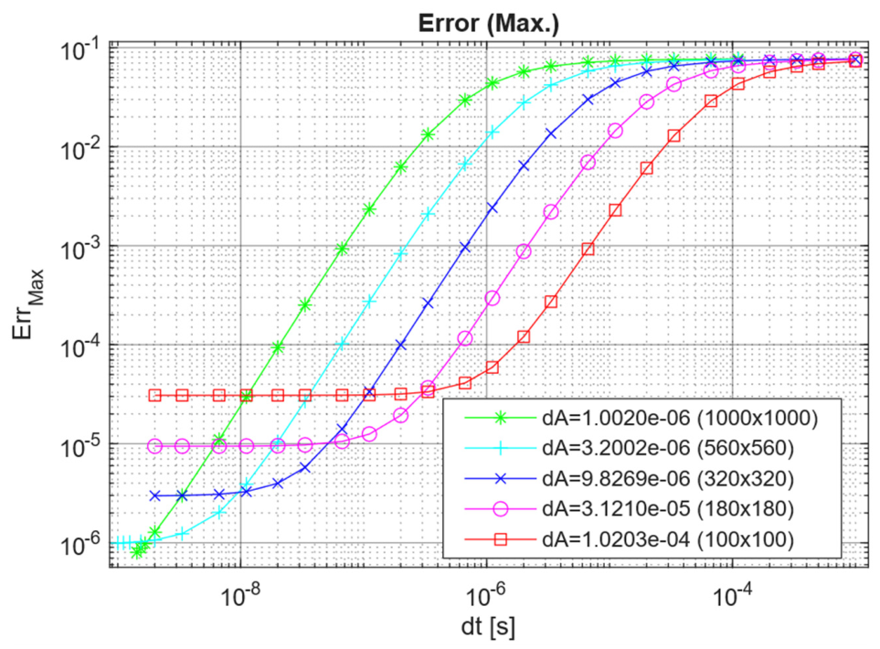
The error vs. timestep size characteristics of the CpC method can be seen in Figure 23.

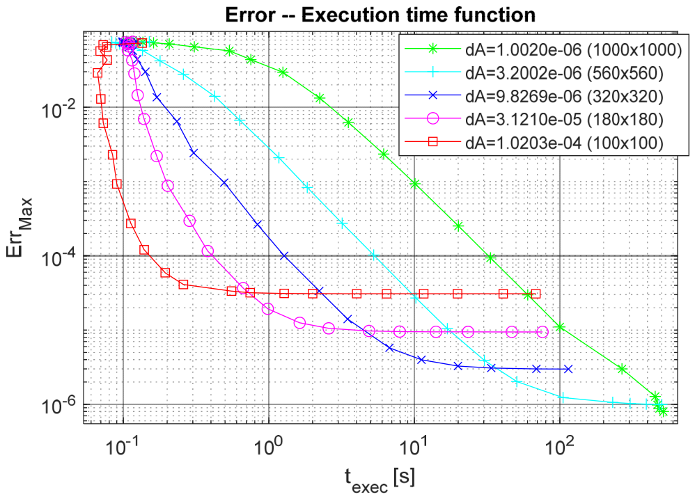
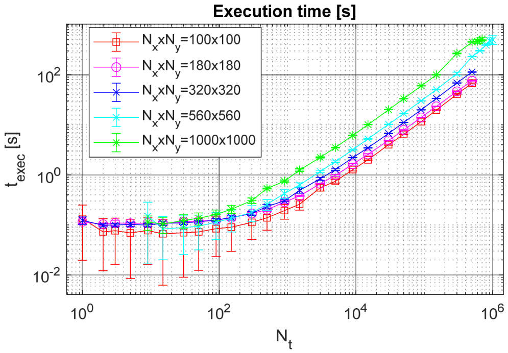
The error is also plotted as a function of the computation time in Figure 24. Similarly, the computation time itself is plotted as a function of the timestep size in Figure 25.

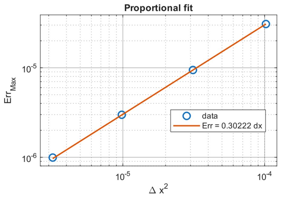
In Figure 23, the asymptote of the 1000 × 1000 curve cannot be seen. To give an estimation of the asymptotic value, we will use the fact that the leading error term of the centered difference formula on a symmetric mesh is:

$${\displaystyle \frac{{∆x}^2}{12}}·\left({\displaystyle \frac{{\partial }^{2}u}{{\partial x}^4}}+{\displaystyle \frac{{\partial }^{2}u}{{\partial y}^4}}\right),$$

(29)

therefore, we know that the residual error value is proportional to ∆x², i.e., the second power of the spatial step-size. The known values are considered by the authors as the last value of the error curves, as presented in

Table 15. Known and unknown asymptotic values of curves of Figure 24.

Spatial Grid	Nr	Δx2	Last Value of ErrMax
100 × 100	10,000	1.020 × 10−4	3.083 × 10−5
180 × 180	32,400	3.121 × 10−5	9.444 × 10−6
320 × 320	102,400	9.827 × 10−6	2.984 × 10−6
560 × 560	313,600	3.200 × 10−6	9.922 × 10−7
1000 × 1000	1,000,000	1.002 × 10−6	<unknown>

.

After plotting the values on a graph, we apply proportional fitting using the model k·∆x², as shown in Figure 26.

The k fitting parameter—along with other statistical values—is shown in

Table 16. Data of proportional fit of Figure 26.

k	R2	RMSE
3.022 × 10−1	0.9999982243	1.577 × 10−8

.

According to these data, the unknown residual error value can be calculated as:

Err_Max(∆x = 1.002 × 10⁻⁶) ≈ 3.022 × 10⁻¹ × 1.002 × 10⁻⁶ = 3.028 × 10⁻⁷.

The last data point of the 1000 × 1000 curve has a value of 7.998 × 10⁻⁷, meaning that only a factor of 2.64 is missing from convergence.

6.3. Discussion

As mentioned before, the variable Dirichlet conditions were implemented by pre-calculating the whole time-evolution of the boundary data. For the applied grid with node count N_x × N_y = 1000 × 1000, there are N_bnd = 2·(N_x − 2) + 2·(N_y − 2) + 4 = 3996 boundary data points. With 64-bit double values, it means 31.25 kB of RAM per timestep. Originally, the authors were able to run with N_t = 650,000 timesteps, which required 650,000 × 3996 × 64 bit ≈ 19.35 GB of RAM. When the algorithm was invoked and the C++-based implementation loaded this data into memory from the file, MATLAB kept in memory the original data used to create the file, which doubled this value up to 38.7 GB. This is in the same order of magnitude as the RAM capacity of 64 GB mentioned in Section 3.4. That is why the prohibitive increase in computation time was experienced. The authors have made MATLAB drop this data after writing the boundary file, which frees some memory and enables going up to N_t = 700,000.

7. Summary and Conclusions

In this study, we have continued the benchmarking of three numerical methods (explicit Euler, Cne, and CpC), beginning in one of our former papers. In addition to the general benchmarking process, we have also examined the depletion of the parallel computation capacity of the GPU by simply scaling up the spatial grid and keeping some pivoted timescales. What is more, we have tried to examine the error convergence graph of the CpC algorithm.

Our experiences are in accordance with our former findings, while on the other hand, we gained some further knowledge: for the pivot timescale of N_t = 500 steps, scaling up the spatial grid to N_x ≤ 1.2 × 10⁹ in one dimension and N_r ≤ 1.6 × 10⁹ in two dimensions, an acceleration factor of 5–40 is reachable. However, this factor differs for the different methods, and reproducible non-monotonic variations in execution time were observed at very large spatial problem sizes. The origin of these variations was not investigated by low-level GPU profiling and therefore no specific hardware-level mechanism is attributed to them. In addition, OpenCL only succeeds in achieving acceleration if a threshold value of N_t and N_r is exceeded, which—in the case of the computer used by the authors—turns out to be around N_r ≈ 2.5 × 10⁴ for N_t = 500.

The error convergence curves of the CpC method are in accordance with the theoretical behavior of the central difference formula used to approximate the Laplacian operator in the differential equation. In addition, this study has given the authors a lesson in methodology: By reconsidering the memory management inside the tester code, finer scaling has become available. This highlights the importance of algorithmic design considering the hardware limitations and reflects the fact that the technically observable convergence curve does not necessarily cover the whole theoretical domain when dealing with FDMs.

As a final word, it is safe to say that OpenCL-based parallelization is only viable if there is a sufficiently high timestep count and spatial node count. Under the hardware and implementation conditions examined here, GPU acceleration was not observed for only a few timesteps on systems containing fewer than approximately 10⁶ spatial values. Nevertheless, for a personal computer with 64 GB of RAM, it becomes possible to execute 500 timesteps on 1.6 × 10⁹ double values within a reasonable time.

References

1. Ledford, H. “RAMmageddon” hits labs: AI-driven memory shortage is impacting science. Nature 2026, 651, 861–862. [Google Scholar] [CrossRef] [Scilit] [PubMed]
2. Hundsdorfer, W.; Verwer, J. Numerical Solution of Time-Dependent Advection-Diffusion-Reaction Equations; Springer Series in Computational Mathematics; Springer: Berlin/Heidelberg, Germany, 2003; Volume 33. [Google Scholar] [CrossRef] [Scilit]
3. Beuken, L.; Cheffert, O.; Tutueva, A.; Butusov, D.; Legat, V. Numerical Stability and Performance of Semi-Explicit and Semi-Implicit Predictor–Corrector Methods. Mathematics 2022, 10, 2015. [Google Scholar] [CrossRef] [Scilit]
4. Essongue, S.; Ledoux, Y.; Ballu, A. Speeding up mesoscale thermal simulations of powder bed additive manufacturing thanks to the forward Euler time-integration scheme: A critical assessment. Finite Elem. Anal. Des. 2022, 211, 103825. [Google Scholar] [CrossRef] [Scilit]
5. Gagliardi, F.; Moreto, M.; Olivieri, M.; Valero, M. The international race towards Exascale in Europe. CCF Trans. High Perform. Comput. 2019, 1, 3–13. [Google Scholar] [CrossRef] [Scilit]
6. Reguly, I.Z.; Mudalige, G.R. Productivity, performance, and portability for computational fluid dynamics applications. Comput. Fluids 2020, 199, 104425. [Google Scholar] [CrossRef] [Scilit]
7. Ali, N.H.M.; Abdullah, R.; Lee, K.J. A comparative study of explicit group iterative solvers on a cluster of workstations. Parallel Algorithms Appl. 2004, 19, 237–255. [Google Scholar] [CrossRef] [Scilit]
8. Ewedafe, S.U.; Shariffudin, R.H. On the Parallel Design and Analysis for 3-D ADI Telegraph Problem with MPI. Int. J. Adv. Comput. Sci. Appl. 2014, 5, 18. [Google Scholar] [CrossRef] [Scilit]
9. Temirbekov, A.; Altybay, A.; Temirbekova, L.; Kasenov, S. Development of parallel implementation for the Navier-Stokes equation in doubly connected areas using the fictitious domain method. East.-Eur. J. Enterp. Technol. 2022, 2, 38–46. [Google Scholar] [CrossRef] [Scilit]
10. Xie, J.; He, J.; Bao, Y.; Chen, X. A low-communication-overhead parallel method for the 3D incompressible Navier-Stokes equations. arXiv 2021, arXiv:2104.08863. [Google Scholar] [CrossRef] [Scilit]
11. Colmenares, J.; Galizia, A.; Ortiz, J.; Clematis, A.; Rocchia, W. A Combined MPI-CUDA Parallel Solution of Linear and Nonlinear Poisson-Boltzmann Equation. BioMed Res. Int. 2014, 2014, 560987. [Google Scholar] [CrossRef] [Scilit] [PubMed]
12. Rueda Castillo, D.; Kaya, U.; Richter, T. An explicit time integration method for Boussinesq approximation. Proc. Appl. Math. Mech. 2024, 24, e202400050. [Google Scholar] [CrossRef] [Scilit]
13. Tan, L.; Huang, M.; Ying, W. A GPU-accelerated Cartesian grid method is proposed for solving the heat, wave, and Schrodinger equations on irregular domains. arXiv 2024. [Google Scholar] [CrossRef] [Scilit]
14. De Luca, P.; Fiorillo, G.; Marcellino, L. A GPU-CUDA Numerical Algorithm for Solving a Biological Model. AppliedMath 2025, 5, 178. [Google Scholar] [CrossRef] [Scilit]
15. Łach, Ł.; Svyetlichnyy, D. Advances in Numerical Modeling for Heat Transfer and Thermal Management: A Review of Computational Approaches and Environmental Impacts. Energies 2025, 18, 1302. [Google Scholar] [CrossRef] [Scilit]
16. Bisbas, G.; Nelson, R.; Louboutin, M.; Luporini, F.; Kelly, P.H.J.; Gorman, G. Automated MPI-X Code Generation for Scalable Finite-Difference Solvers. In Proceedings of the 2025 IEEE International Parallel and Distributed Processing Symposium (IPDPS), Milano, Italy, 3–7 June 2025; pp. 689–701. [Google Scholar] [CrossRef] [Scilit]
17. Essongue, S.; Diarra, B.; Lacoste, E. Runge–Kutta–Chebyshev schemes to accelerate thermal modelling of additive manufacturing processes. Finite Elem. Anal. Des. 2026, 256, 104527. [Google Scholar] [CrossRef] [Scilit]
18. Kareem Jalghaf, H.; Omle, I.; Kovács, E. A Comparative Study of Explicit and Stable Time Integration Schemes for Heat Conduction in an Insulated Wall. Buildings 2022, 12, 824. [Google Scholar] [CrossRef] [Scilit]
19. Kovács, E. A class of new stable, explicit methods to solve the non-stationary heat equation. Numer. Methods Partial Differ. Equ. 2021, 37, 2469–2489. [Google Scholar] [CrossRef] [Scilit]
20. Kovács, E.; Nagy, Á.; Saleh, M. A set of new stable, explicit, second order schemes for the non-stationary heat conduction equation. Mathematics 2021, 9, 2284. [Google Scholar] [CrossRef] [Scilit]
21. Koics, D.; Kovács, E.; Hornyák, O. Effects of OpenCL-Based Parallelization Methods on Explicit Numerical Methods to Solve the Heat Equation. Computers 2024, 13, 250. [Google Scholar] [CrossRef] [Scilit]
22. Mátyás, L.; Barna, I.F. General Self-Similar Solutions of Diffusion Equation and Related Constructions. Rom. J. Phys. 2022, 67, 101. [Google Scholar]
23. Garvey, J.D.; Abdelrahman, T.S. A Strategy for Automatic Performance Tuning of Stencil Computations on GPUs. Sci. Program. 2018, 2018, 6093054. [Google Scholar] [CrossRef] [Scilit]
24. OpenCL. Wikipedia. 18 July 2026. Available online: https://en.wikipedia.org/w/index.php?title=OpenCL&oldid=1364852294 (accessed on 7 September 2026).
25. OpenCL. The Open Standard for Parallel Programming of Heterogeneous Systems. The Khronos Group. Available online: https://www.khronos.org/opencl/ (accessed on 7 September 2026).
26. Halbiniak, K.; Szustak, L.; Olas, T.; Wyrzykowski, R.; Gepner, P. Exploration of OpenCL Heterogeneous Programming for Porting Solidification Modeling to CPU-GPU Platforms. Concurr. Comput. Pract. Exp. 2021, 33, e6011. [Google Scholar] [CrossRef] [Scilit]
Figure 1. Scheme of Euler (top-left), CNe (top-right), and CpC (bottom) methods.
Computers 15 00673 g001
Figure 2. Using GPU memory buffers with Euler and CNe method.
Computers 15 00673 g002
Figure 3. Using GPU memory buffers with the 2nd stage of CpC.
Computers 15 00673 g003
Figure 4. The initial function and reference solution used with 1-dimensional CNe and CpC methods.
Computers 15 00673 g004
Figure 5. The initial function (a) and reference solution (b) for Tinit = 0.1 and Tfin = 0.2.
Computers 15 00673 g005
Figure 6. A 3D illustration of the analytical solution for t = 0.071.
Computers 15 00673 g006
Figure 7. The error of the 1D computations, as a function of the execution time.
Computers 15 00673 g007
Figure 8. The error of the 1D computations, as a function of the timestep size.
Computers 15 00673 g008
Figure 9. The error of the 2D computations, as a function of the execution time.
Computers 15 00673 g009
Figure 10. The error of the 2D computations, as a function of the timestep size.
Computers 15 00673 g010
Figure 11. Computation time of the sequential CpC for different 1D spatial grids, as a function of the timestep count, with error bars.
Computers 15 00673 g011
Figure 12. Computation time of the OpenCL-based CpC for different 1D spatial grids, as a function of the timestep count.
Computers 15 00673 g012
Figure 13. Computation time of the sequential CpC for different 2D spatial grids, as a function of the timestep count.
Computers 15 00673 g013
Figure 14. Computation time of the OpenCL-based CpC for different 2D spatial grids, as a function of the timestep count.
Computers 15 00673 g014
Figure 15. Computation time of different implementations of CpC, as a function of the spatial node count, for Nt = 1.
Computers 15 00673 g015
Figure 16. Computation time of different implementations of CpC, as a function of the spatial node count, for Nt = 5.
Computers 15 00673 g016
Figure 17. Computation time of different implementations of CpC, as a function of the spatial node count, for Nt = 50.
Computers 15 00673 g017
Figure 18. Computation time of different implementations of CpC, as a function of the spatial node count, for Nt = 500.
Computers 15 00673 g018
Figure 19. Computation time of different implementations of CpC, as a function of the spatial node count, for Nt = 5000.
Computers 15 00673 g019
Figure 20. Computation time of different implementations of CpC, as a function of the spatial node count, for Nt = 50,000.
Computers 15 00673 g020
Figure 21. Computation time of different implementations of CpC, as a function of the spatial node count, for Nt = 200,000.
Computers 15 00673 g021
Figure 22. The computation time, as a function of the total number of spatial grid-points, for 500-timestep computations, scaling up to a spatial grid-point count of 1.6 × 10⁹.
Computers 15 00673 g022
Figure 23. The algorithmic error of the CpC method, as a function of the timestep size.
Computers 15 00673 g023
Figure 24. The algorithmic error of the CpC method, as a function of the execution time.
Computers 15 00673 g024
Figure 25. The computation time of the CpC method, as a function of the timestep count.
Computers 15 00673 g025
Figure 26. The known asymptotic values of Figure 23, as a function of the spatial step-size along the x-axis squared, along with the fitted line of proportion.
Computers 15 00673 g026