Article

Machine Learning-Based Gallstone Prediction Using Clinical Markers and Multiple Explainable AI Methods


by
Abhijay N. Sampathila
,
Krishnaraj Chadaga
*,
Devadas Bhat
and
Niranjana Sampathila
*
Manipal Institute of Technology, Manipal Academy of Higher Education, Manipal 576104, India
*
Authors to whom correspondence should be addressed.
Computers 2026, 15(10), 668; https://doi.org/10.3390/computers15100668
Submission received: 5 July 2026 / Revised: 12 September 2026 / Accepted: 14 September 2026 / Published: 1 October 2026
(This article belongs to the Special Issue Deep Learning and Explainable Artificial Intelligence (2nd Edition))

Abstract

Gallstones, also known as cholelithiasis, are hardened deposits of bile (digestive fluid) formed in the gallbladder. Gallstones are a common gastrointestinal condition. They often lead to complications like cholecystitis, biliary obstruction, and pancreatitis. The diagnosis of gallstones involves blood tests, ultrasonography, and Computed Tomography (CT)/Magnetic Resonance Imaging (MRI) scans. Artificial intelligence (AI) and machine learning (ML) have revolutionized medical diagnostics and have led to an increase in the precision and efficiency of diagnosis. In this research study, multiple supervised learning techniques were used to predict the presence of gallstones in patients. The three hyperparameter tuning techniques utilized to optimize predictive performance include: grid search algorithm, randomized search algorithm and Bayesian optimization. The randomized search algorithm performed the best among the three, with an accuracy of 83%. The AdaBoost Classification and the CatBoost Classification techniques were top performers amongst the nine learning techniques utilized in this study. The customized ensemble (stacking) model achieved an F1-score of 84% (95% CI: 71.2–91.8%) and had an AUC of 0.90 using the randomized search algorithm. Further, eight Explainable Artificial Intelligence (XAI) techniques were utilized to interpret the classification results. Vitamin D and C-Reactive Protein (CRP) were identified as the most influential factors in predicting the condition, by XAI techniques. This highlights their significant role in predictive accuracy. The proposed model demonstrates its ability to assist healthcare professionals. It would enable efficient validation of the results obtained from other diagnostic methods.

1. Introduction

Gallstones are primarily caused due to an imbalance in the composition of bile [1]. They lead to the crystallization of cholesterol or bilirubin. This imbalance can result from numerous factors like high cholesterol/bilirubin levels in bile, insufficient bile salts or improper emptying of the gallbladder. Obesity, rapid weight loss and a diet consisting of high fat and low fiber can increase the chances of gallstone formation [2]. The dietary factors that increase the chances of gallstone formation include cholesterol, saturated fat, trans fatty acids, and refined sugar [3]. Hence, it is advised to avoid them in a diet. Consuming polyunsaturated fat, monounsaturated fat, and fiber may help in preventing the formation of gallstones. Following a vegetarian diet can reduce the risk of gallstones. Additionally, some nutritional supplements like Vitamin C, soy lecithin, and iron might be beneficial.
The conventional treatment for symptomatic gallstones includes cholecystectomy, surgical removal of the gallbladder [4]. It often resolves symptoms, even though 10–15% of patients may develop post-cholecystectomy syndrome. The other method involves oral administration of bile acids like ursodeoxycholic acid or chenodeoxycholic acid. These dissolve radiolucent gallstones over several months to two years but may cause gastrointestinal side effects. This method has a high recurrence rate after treatment discontinuation [4]. Lithotripsy may be used with ursodeoxycholic acid for single, non-calcified gallstones.
Gallstones, particularly cholesterol gallstones, can lead to various gastrointestinal symptoms and pose a risk of acute or chronic cholecystitis [5]. Gallstones are usually asymptomatic, but some patients experience biliary colic characterized by sudden and severe right-upper-quadrant pain often with nausea and vomiting. The complications of cholecystitis can include infection, perforation, and gangrene.
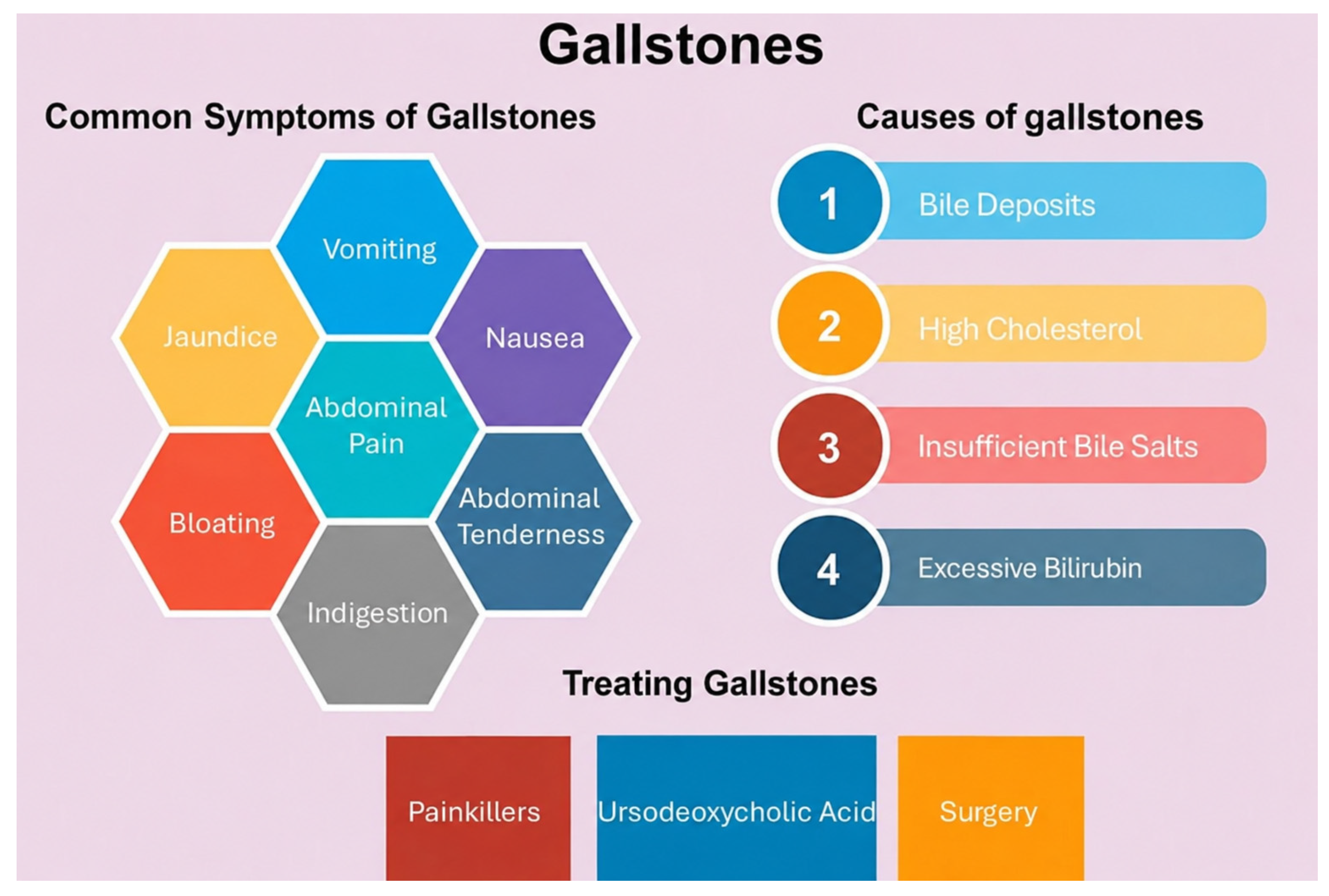
Machine learning (ML) and Explainable Artificial Intelligence (XAI) play a crucial role in enhancing gallstone prediction, by improving diagnostic accuracy and efficiency. ML algorithms analyze patient data including lab results and cholesterol levels, to identify patterns indicative of gallstone formation. Techniques like Random Forest and gradient boosting can effectively classify patients based on risk factors. XAI methods such as Shapley Additive Values (SHAP) and Local Interpretable Model-Agnostic Explanations (LIME) help clinicians understand the physiological features that increase the chance of gallstone formation. Figure 1 is a pictorial representation of common symptoms of gallstones, causes of gallstones and the treatment for gallstones.
A few studies exist that use ML for gallstone detection. Laifu Deng et al. [6] used ML and logistic regression (LR) models to predict gallstones. The dataset was obtained through the National Health and Nutrition Examination Survey (NHANES). The logistic regression model achieved the highest accuracy of 68.1% amongst the four tested algorithms. Yuhu Ma et al. [7] used ML techniques on Computed Tomography (CT) features and clinical data to predict the severity of acute gallstone pancreatitis. The Random Forest method was used in the model. The model achieved an accuracy of 84.6% in predicting the severity of acute gallstone pancreatitis. Khadija M Jack et al. [8] used machine learning (ML) and deep learning (DL) techniques to identify clinical and metabolomic features associated with gallstone disease. The Support Vector Machine (SVM) and Random Forest (RF) algorithms were used to classify the presence of gallstones. This model achieved the highest prediction accuracy of 83%. MD Irfan Esen et al. [9] suggested a machine learning-based prediction model for gallstone disease utilizing bioimpedance and laboratory data. They obtained the highest accuracy of 85.42% for the gradient boosting technique. The findings of various other studies have been tabulated in Table 1.
There were certain unexplored areas in the publicly accessible studies. Most studies lacked the use of multiple XAI techniques. This highlights the need for visual interpretation of the predictions. In several studies, XAI techniques were limited to the use of SHAP and LIME explainers. Other newer XAI techniques could be used to improve the interpretability of model results.
On the contrary, this study optimized interpretable machine learning algorithms to predict gallstone disease among patients and identify the potential risk factors. Eight XAI tools and methodologies were used to describe the model outputs in detail. This research makes the following contributions:
  • Three hyperparameter optimization techniques have been utilized and compared to enhance the classifiers. They are: (a) randomized search, (b) grid search and (c) Bayesian optimization.
  • The ensemble model was customized by stacking nine different models. This has increased the precision, recall, and F1-score and has also made the prediction of gallstones more accurate.
  • The eight XAI techniques, namely, SHAP, LIME, QLattice, Partial Dependence Plots (PDPs), Individual Conditional Expectations (ICEs), Eli5, anchor and counterfactual explanations make the predictions comprehensible, interpretable, and transparent. No one study exists that uses eight different XAI techniques for gallstone prediction. Explainers such as anchor and counterfactual explanations have rarely been used in ML research.

2. Materials and Methods

2.1. Dataset

This clinical data was collected from the Internal Medicine Outpatient Clinic of Ankara VM Medical Park Hospital, Turkey and is freely accessible on the UCI Machine Learning Repository [9]. This dataset contains 38 features, including demographic, bioimpedance, and laboratory data. It includes the data from 319 individuals out of which, 161 had gallstones. The presence or absence of gallstones along with all clinical, bioimpedance, and laboratory parameters was documented in one single patient visit, hence making it suitable for a retrospective classification of gallstone status instead of the prediction of the future development of gallstones. This increases the feature-to-sample ratio. This study aims to develop an ML- and XAI-based model that accurately predicts gallstone disease. The below table represents the brief description of each marker. Table 2 presents a description of markers used in this study to predict gallstones. The original source does not report a specific recruitment period or detailed inclusion and exclusion criteria beyond outpatient status. Comorbidities are captured directly as model features (Table 2). The target variable ‘Gallstone Status’ was coded such that 1 indicates the presence of gallstones (positive class, 161) and 0 indicates the absence of gallstones (158). This coding was used consistently throughout all model training, evaluation, and XAI interpretation reported in this study.

2.2. Statistical Analysis and Data Preprocessing

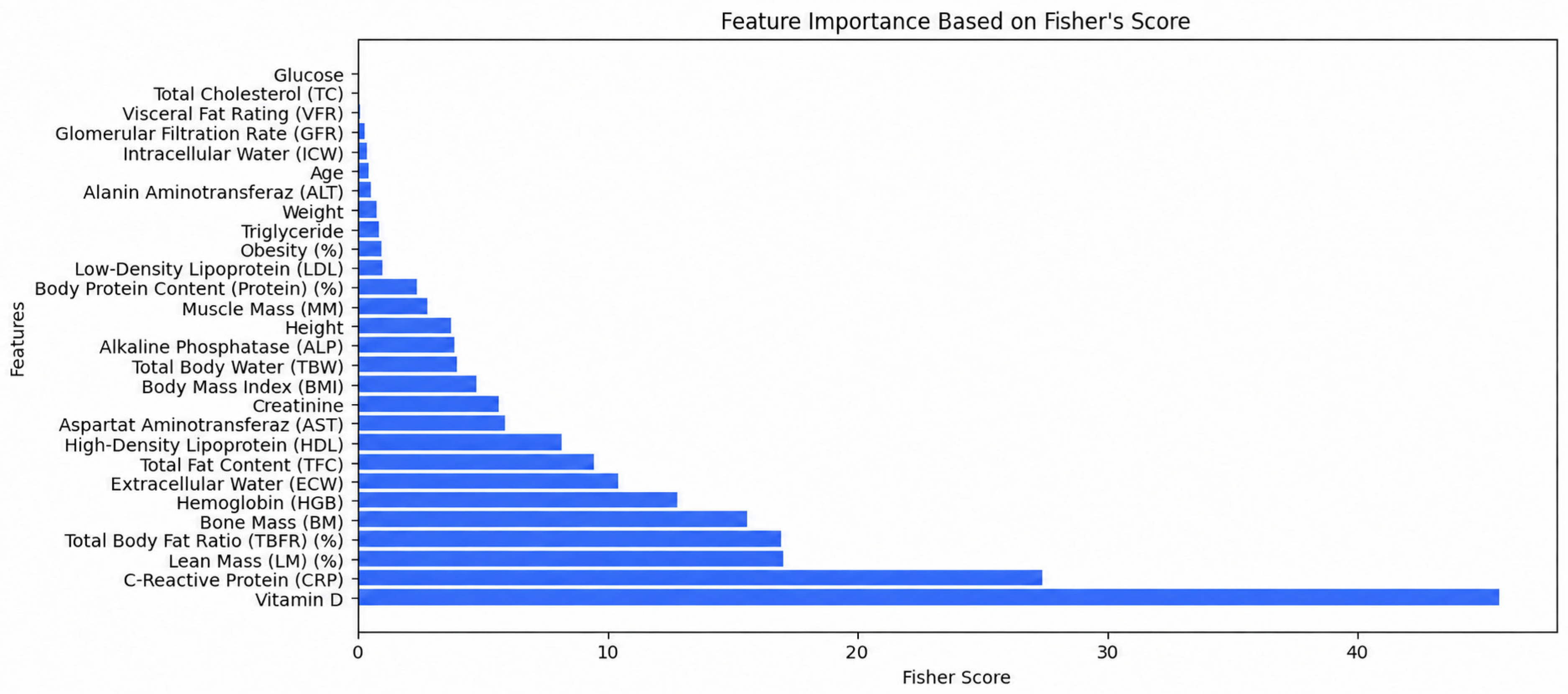
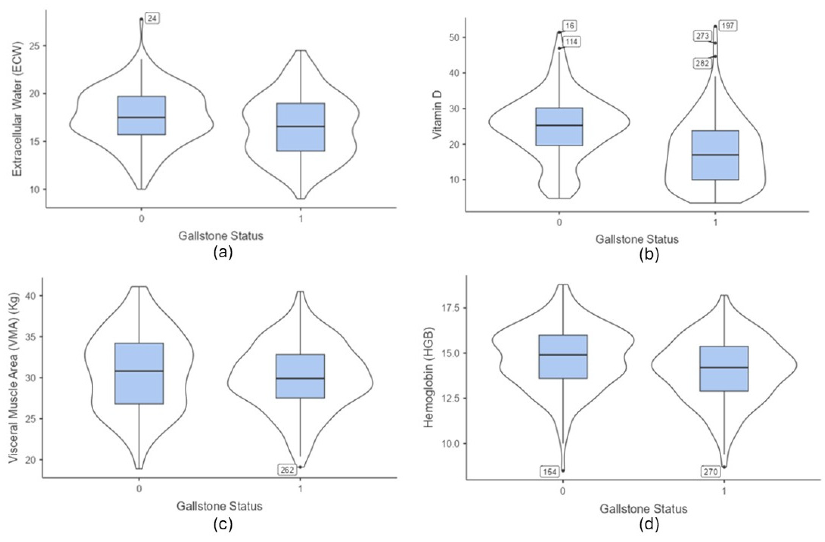
The dataset was balanced and free of null values. Further, descriptive and inferential statistical analysis was conducted on the dataset to identify key parameters. The parameters for the descriptive statistical analysis of continuous attributes have been plotted in Table 3. Inferential statistical analysis was performed through t-tests and chi-square tests. If the p-value is less than 0.001, then it is an important attribute in gallstone prediction. The univariate test was utilized as a preliminary screen procedure. Significant univariate results do not necessarily mean that the variables are important for the multivariate models, which are evaluated by Fisher’s score and XAI analyses. The results of Student’s t-test are described below in Table 4. The results of chi-square tests on categorical attributes are depicted in Table 5. Data is usually scaled to avoid potential biases [14]. The dataset was split into training (80%, n = 255) and test (20%, n = 64) sets. All data-dependent preprocessing steps, including Standard Scaler and categorical encoding, were fit exclusively on the training set. Fisher’s score feature ranking was computed on the training set. These steps were implemented within a scikit-learn pipeline, refit separately within each cross-validation fold during hyperparameter tuning, ensuring no information from validation folds or the held-out test set influenced preprocessing or model selection. The test set was reserved exclusively for final performance evaluation, reported in Table 6. The Standard Scaler was used to scale the data and ensure that the features are standardized to zero mean and unit variance. All categorical variables (Gender, Comorbidity, Coronary Artery Disease, Hypothyroidism, Hyperlipidemia, Diabetes Mellitus) were retained in their original numeric coding and used alongside the continuous features without additional transformation. The full feature matrix therefore comprised the 38 variables listed in Table 2. Fisher’s score was computed using ANOVA F-statistics, depicted in Figure 2. Vitamin D, C-Reactive Protein (CRP), Lean Mass (LM), Total Body Fat Ratio (TBFR), and Bone Mass (BM) were found to be the key features in predicting gallstone disease, based on Fisher’s score. For the XAI techniques like SHAP and LIME, the top 20 continuous features ranked by Fisher’s score were considered. This subset excludes the categorical/binary clinical variables and Hepatic Fat Accumulation (HFA), which were not included in the ranked continuous feature selection. Hyperparameter tuning was performed using randomized search CV via cross-validation folds drawn from the training set to optimize the model. The model was internally validated through a train–test and cross-validation approach. The attributes were compared using violin plots, as shown in Figure 3. It can be seen that there was a significant difference in Vitamin D levels between the two cohorts.

2.3. Machine Learning and XAI Techniques

In this study, an ensemble model was customized through stacking. It combined nine base learners including Random Forest, logistic regression, KNN, SVM, Decision Tree, AdaBoost, CatBoost, XGBoost and gradient boosting. This model provides an effective technique for improving predicting performance. Stacking enhances prediction effectiveness by the combination of the predictive capacity of different classifiers using a meta-learner [15]. Combining multiple models helps in minimizing the overfitting. In this study, the meta-learner is a logistic regression model (final_estimator), trained on out-of-fold predicted probabilities from the nine base learners, generated via 5-fold internal cross-validation (cv = 5, stack_method = ‘predict_proba’) so that no base learner ever produces a training meta-feature from data it was trained on. The meta-learner receives only these probability outputs, not the original 38 features. The default threshold of 0.5 was used for final classification. This architecture was used to leverage diverse model strengths, minimizing individual weaknesses. The full mathematical formulations of the nine base learners and the stacking meta-learner are provided in Appendix A.
Eight XAI techniques were used to interpret the predictions made by algorithms. They were:
  • SHapley Additive exPlanations (SHAP): It is a technique based on game theory that can be used to understand the outcomes of any classifier [16]. This approach applies game theory’s Shapley values to determine the optimal credit allocation based on local factors. The SHAP values distribute the outcome value across attributes for an estimation. The SHAP value assigned to each attribute represents its contribution to the definitive foresight.
  • Local Interpretable Model-Agnostic Explanation (LIME): It produces interpretable features by discretizing each dimension [17]. It is an agnostic model and supports a wide range of ML algorithms.
  • Partial Dependence Plots (PDPs): They show how the values of a feature or pair of features impact a model’s predictions [18]. They estimate the average effect of a predictor variable on the predictive variable.
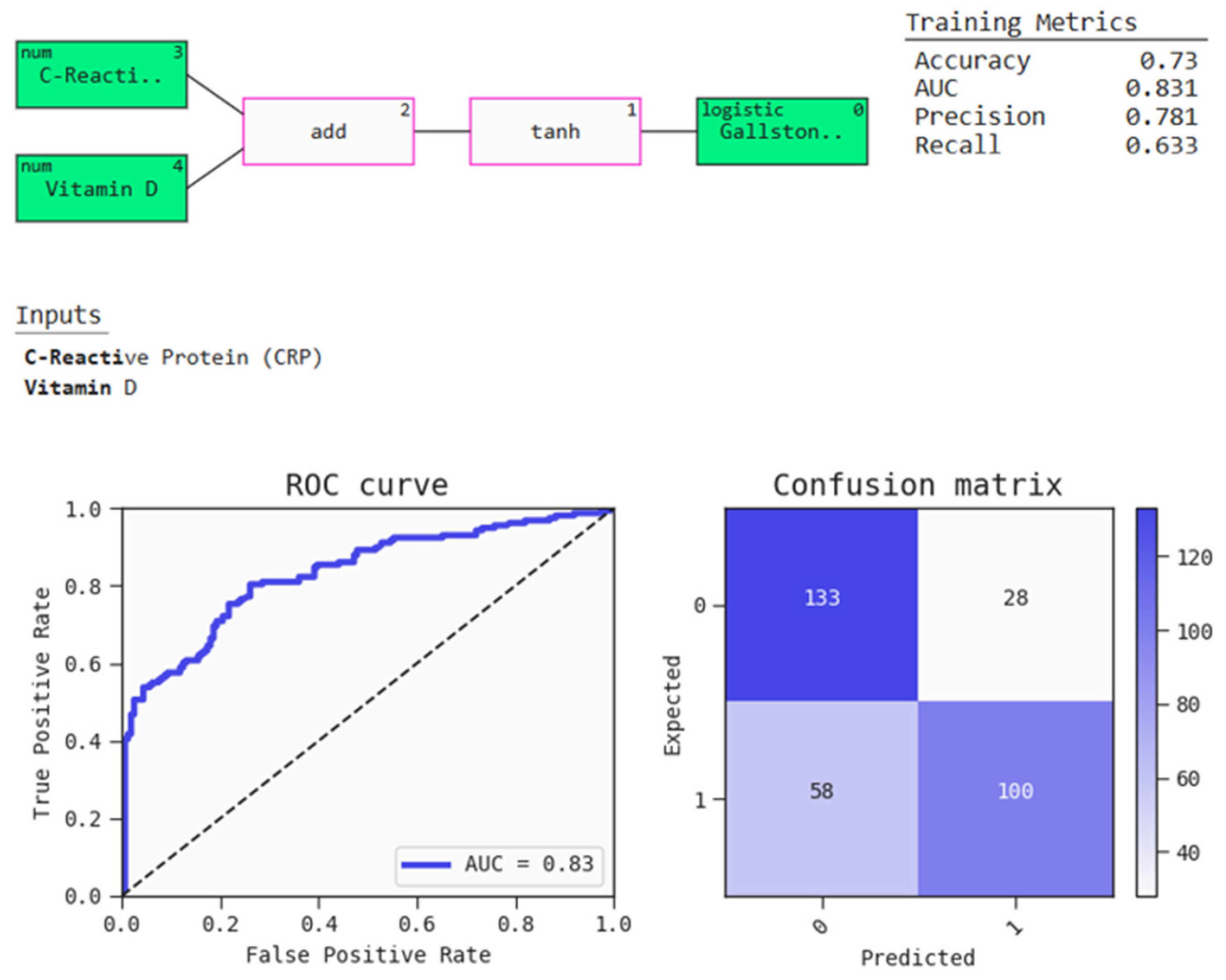
  • QLattice: ‘Abzu’ developed QLattice in 2018 [19]. It utilizes the concept of symbolic regression. Both numerical and categorical attributes can be entered as the input. The model explanation is created with QGraphs. They include activation functions, edges, and nodes. The activation function alters the output, connecting nodes and representing each attribute with a node.
  • Individual Conditional Expectation (ICE): ICE plots depict the variation in the fitted values. They suggest where and to what extent heterogeneities exist [20]. They disaggregate the averaged data, allowing researchers to analyze the effect of the predictor variable at each value level while maintaining the values of the other predictor variables constant.
  • Explain Like I am 5 (Eli5): Eli5 is a Python package that explains the predictions made by an algorithm [21]. It supports a diverse set of machine learning algorithms. It can successfully manage small consistency issues. Additionally, it facilitates code reuse. It is well known that Eli5 can manage both local and global interpretation.
  • Anchor: The anchor method offers explanations that are specifically customized to the model’s behavior within the identical perturbation space, resulting in enhanced accuracy and transparency [22]. It provides simple rule-based explanations for complex models by identifying stable prediction conditions. It is useful for decision-making in scenarios where trust and clarity are crucial.
  • Counterfactual Explanation: A counterfactual explanation indicates what should have changed in an event for observing a different outcome [23]. It depicts how certain changes to an input could lead to a different outcome.
Hyperparameter optimization is crucial in machine learning to improve data accuracy. Searching techniques are used to determine the appropriate hyperparameters for each algorithm. The three techniques used to identify the crucial parameters in this study are as follows:
  • Grid Search: It involves defining a grid of hyperparameters. Each combination in the grid is carefully analyzed and evaluated [24]. This method involves the process of defining the hyperparameter grid, training and evaluating the model. Optimal hyperparameters are selected and the model is validated.
  • Randomized Search: It works faster and more efficiently in high-dimensional spaces [25]. It samples the hyperparameters from specific distributions. This technique includes defining hyperparameter distributions, random sampling, training and evaluating models, selecting optimal hyperparameters, and validating the models.
  • Bayesian Optimization: Hyperparameters are selected through Bayes’ theorem [26]. An acquisition function balances the exploration and exploitation stages of the search process after the search space is defined.

3. Results

3.1. Classification Results

A total of three hyperparameter tuning techniques (grid search, randomized search, and Bayesian optimization) were compared for each of the nine base learners under an identical protocol (five-fold stratified cross-validation, random_state = 42). These hyperparameter tuning techniques were utilized to find the best set of hyperparameters. The tuning strategy selection was based on cross-validation within the training set. F1-score was chosen to be the primary evaluation parameter for model performance because it considers both the precision and the recall together. This makes it highly suitable for an imbalanced medical dataset where false positives and false negatives have medical relevance.
Table 6 presents the classification results. When the grid search technique was used, Hard Voting gave the best results with the highest accuracy and F1-score of 86%. It also had the lowest Hamming Loss of 0.14 and highest Jaccard score of 0.74, implying that it made the fewest mistakes overall. XGBoost had the highest AUC of 0.91, slightly better than CatBoost and Soft Voting, which both scored 0.89. However, XGBoost’s accuracy of 80% was lower than Hard Voting’s. When the randomized search technique was used, Soft Voting and the stacking model both achieved the highest accuracy and F1-score of 84%. The stacking model also had the best MCC of 0.69 and Jaccard score of 0.73 in this group, showing that its predictions were more balanced and reliable. CatBoost had the highest AUC of 0.91, just ahead of stacking, Soft Voting, and XGBoost, which all scored 0.90. Using the Bayesian optimization technique, Soft Voting performed best, with the highest accuracy and F1-score of 84%, ahead of the stacking model, which scored 80% on both. CatBoost, XGBoost, and stacking all shared the highest AUC of 0.90.
The stacking model tuned via randomized search achieved a strong and balanced performance, with an F1-score of 84% (95% CI 71.2–91.8%), an accuracy of 83%, and an AUC of 0.90. The model demonstrated a sensitivity of 83%, a specificity of 70%, a positive predictive value of 83%, and a negative predictive value of 80%.
While Soft Voting achieved a comparable accuracy and F1-score under randomized search, its underlying mechanism is comparatively simple. It aggregates predictions by averaging the outputs of individual learners, without considering the reliability of each learner. It leads to a weak model and a strong model contributing equally to the final decision. Stacking, on the other hand, uses a meta-learner trained on the out-of-fold predicted probabilities of the base learners across five folds. This allows the meta-learner to identify which base models are more trustworthy under different conditions and weight their contributions accordingly, rather than treating all learners as equally reliable. This distinction is reflected in the stacking model’s higher MCC and Jaccard score compared to Soft Voting, suggesting more consistent and better calibrated predictions rather than accuracy driven by a few dominant learners.
Among the three hyperparameter tuning strategies, the stacking model under randomized search was selected for further analysis, including XAI, as it offered the most balanced performance across accuracy, F1-score, MCC, and Jaccard score. It outperformed its grid search and Bayesian optimization counterparts on these combined metrics. This balance was prioritized over any single metric, since a model that performs well across multiple evaluation criteria is more likely to generalize reliably and produce trustworthy explanations in downstream interpretability analysis.
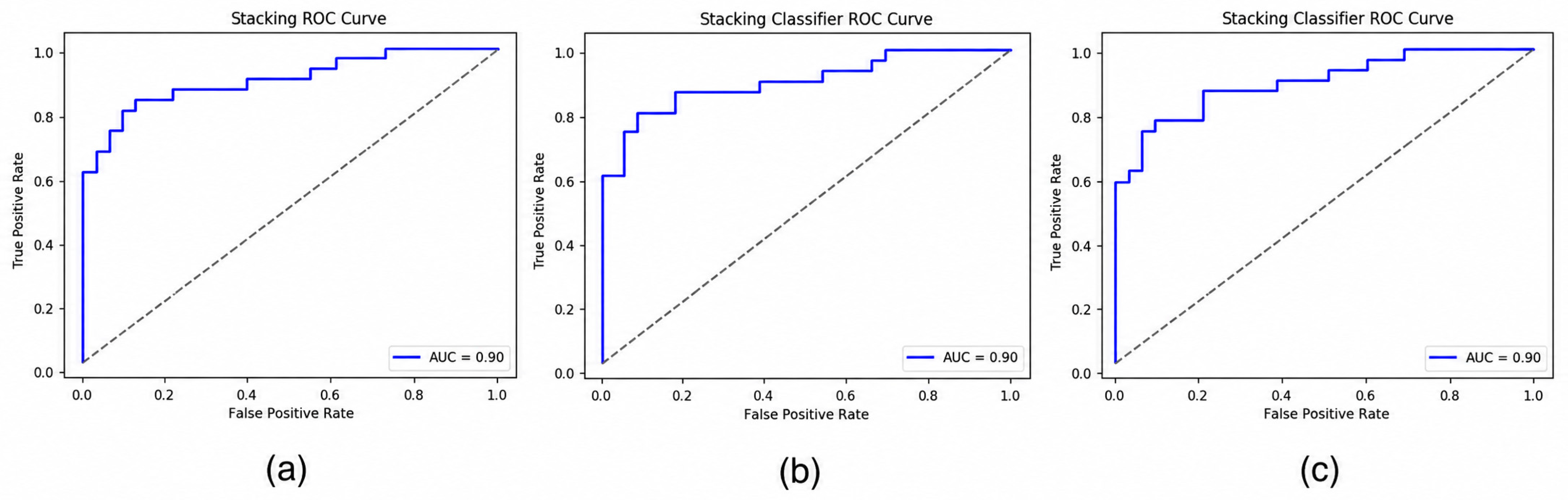
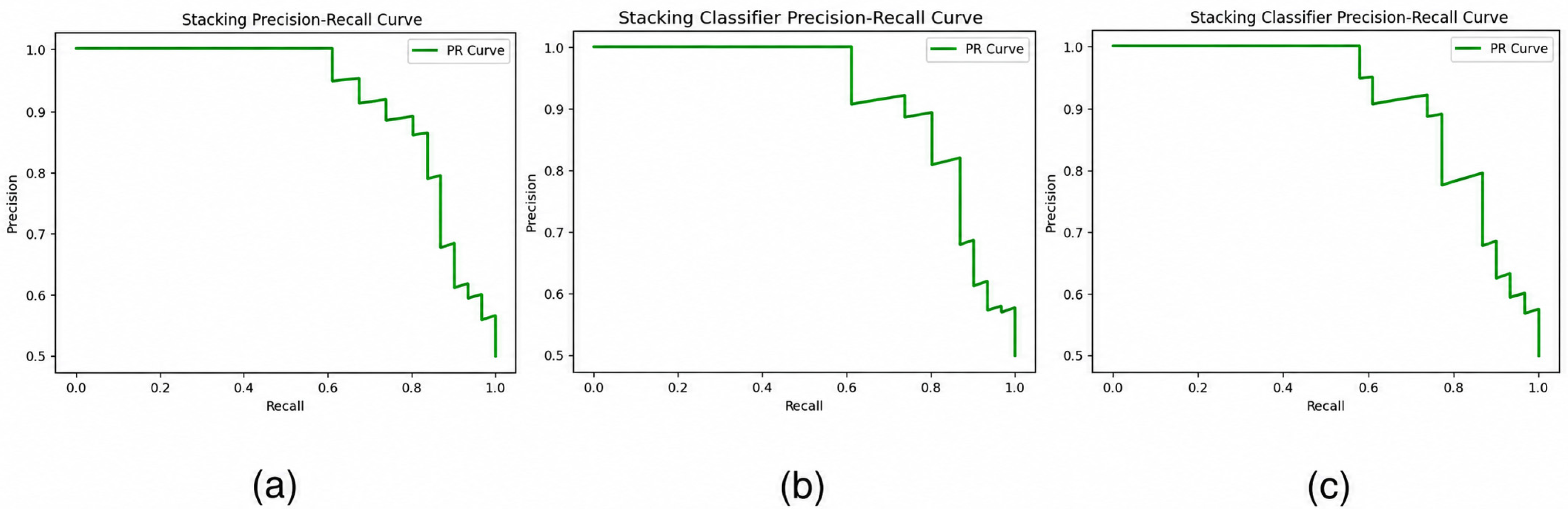
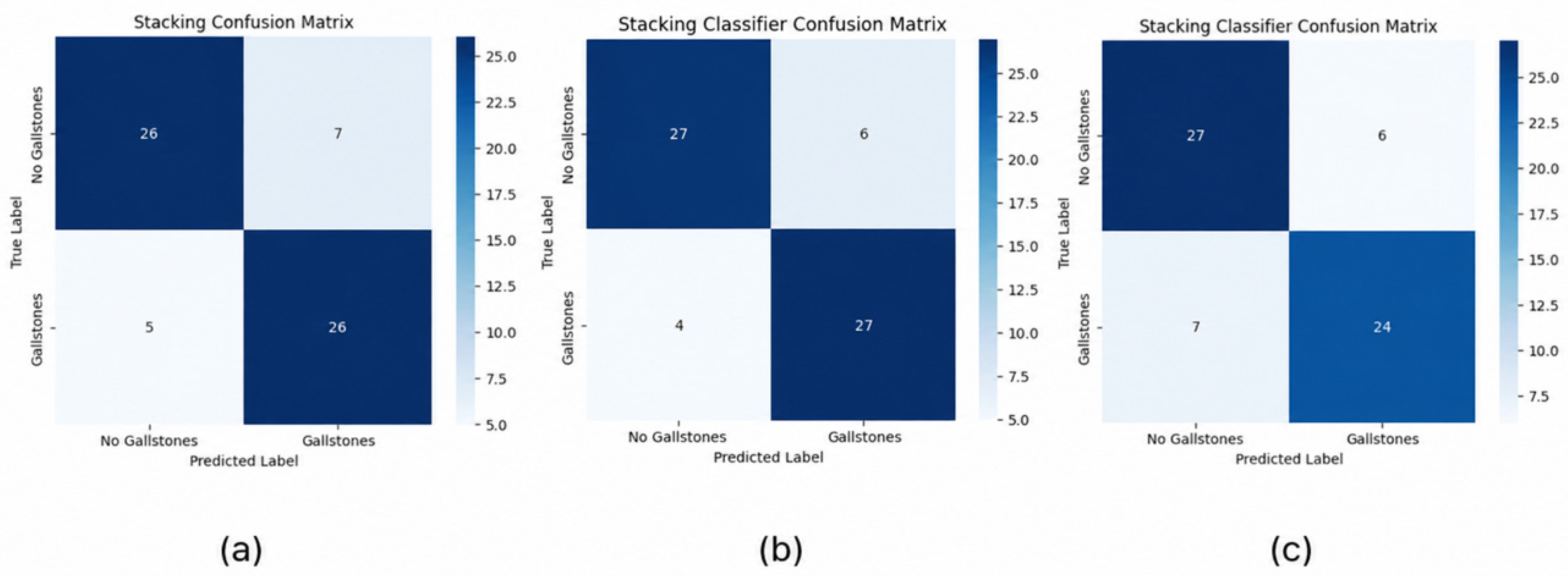
Full search spaces, configuration counts, and cross-validated F1-scores for all three strategies are reported in Table 7. Randomized search was selected as the tuning strategy for the final reported models and subsequent XAI analysis, based on its performance relative to the other two strategies within a comparable computational budget. The hyperparameters selected by various algorithms for the randomized search technique are tabulated in Table 7. Figure 4 is a depiction of the Receiver Operating Characteristic (ROC) curve for all the customized ensemble models. Figure 5 depicts the precision–recall (PR) curve for all customized ensemble models. There were very few false positives and false negative instances. This indicates accurate prediction. Figure 6 depicts the confusion matrices of the stacking model for the three hyperparameter tuning strategies. Algorithms obtained satisfactory results by preprocessing and balancing the data and utilizing hyperparameters.
A baseline logistic regression model was trained using established risk factors for gallstones (age, gender, BMI, and Total Cholesterol). On testing, the model achieved an accuracy of 56% and an AUC of 0.60. In addition to the baseline model, we examined the penalized (L2) logistic regression with all 38 variables following the same procedure, with accuracy being 83%, F1-score being 84%, and AUC equal to 0.90. In order to estimate the contribution of CRP and Vitamin D, we compared the full model above with a model involving one fewer predictor, i.e., CRP and Vitamin D removed from consideration (36 variables). The latter model demonstrated a lower level of accuracy at 73.62%. The likelihood ratio test for the nested models was highly significant (LR = 36.12, df = 2, p < 0.001).

3.2. XAI Analysis

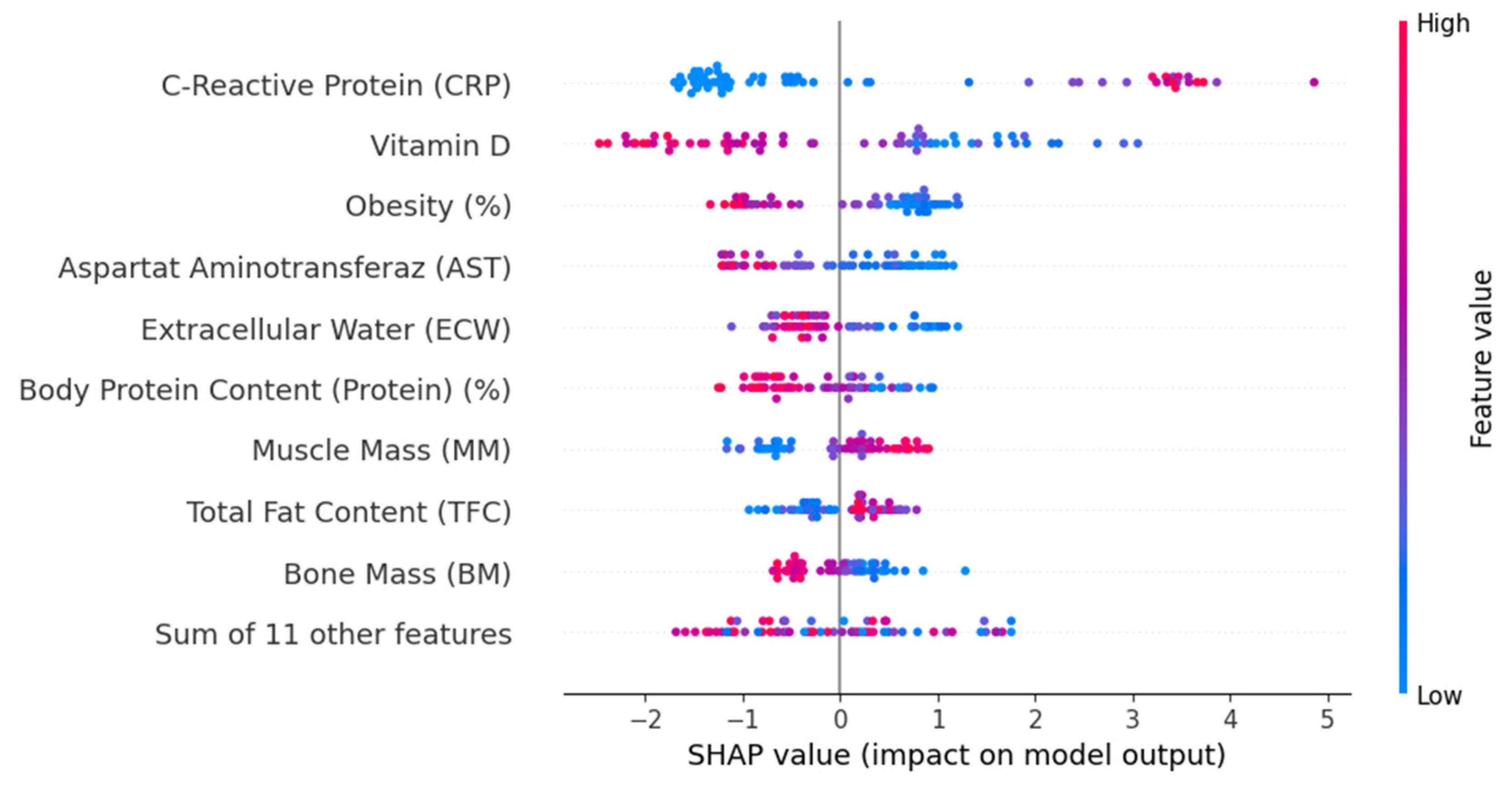
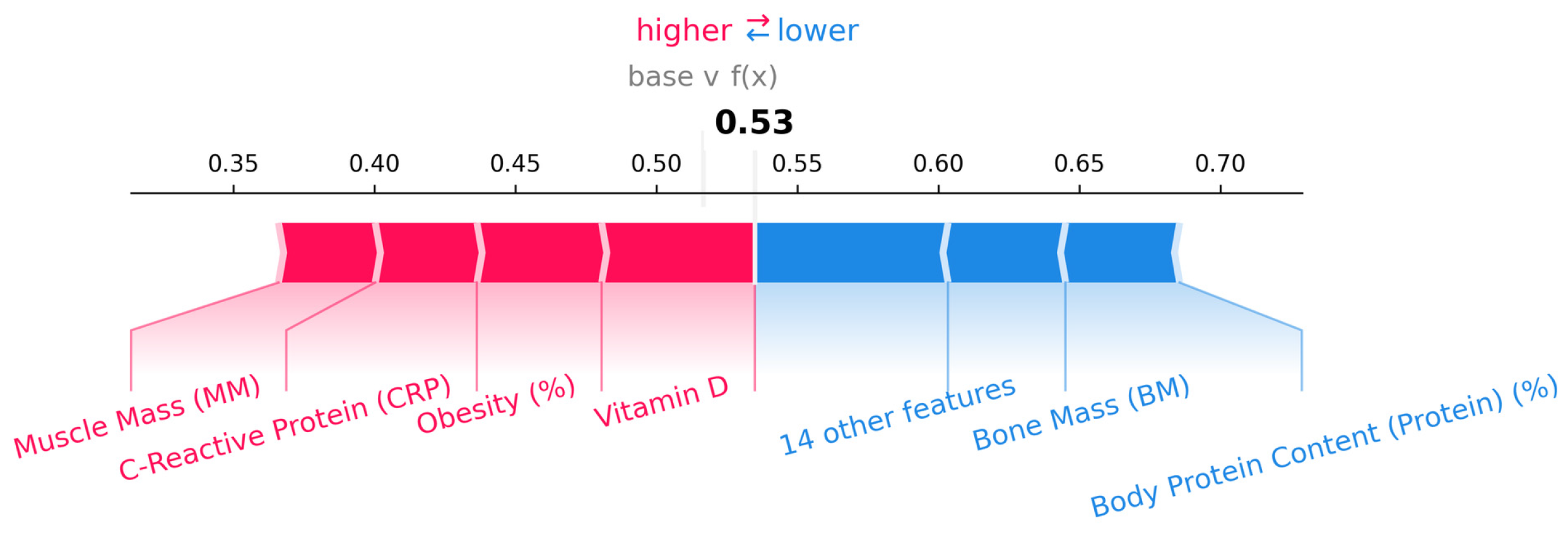
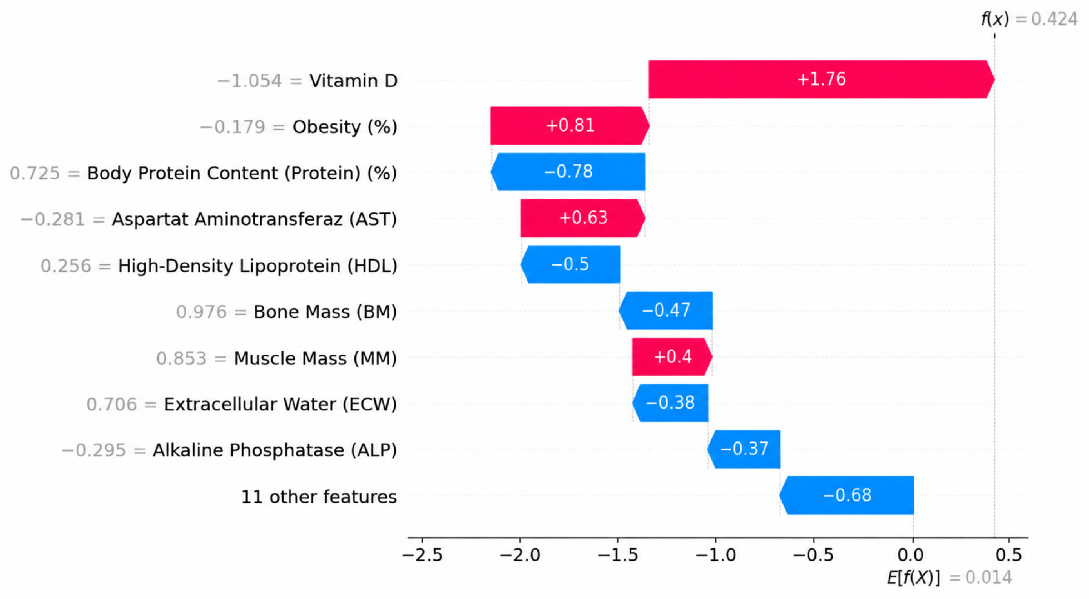
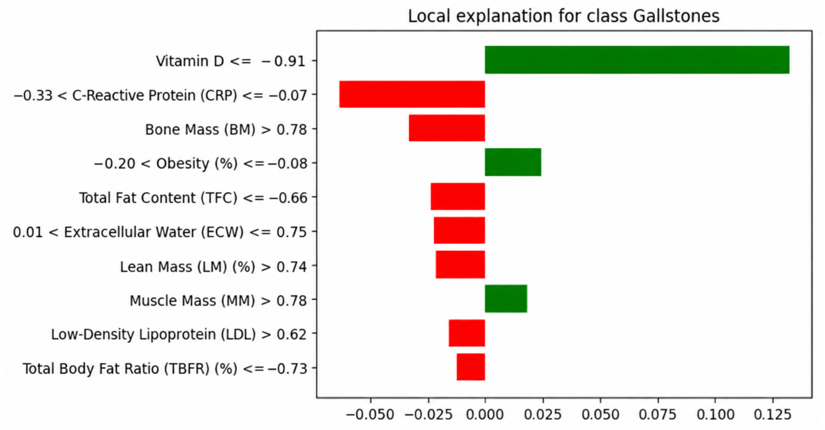
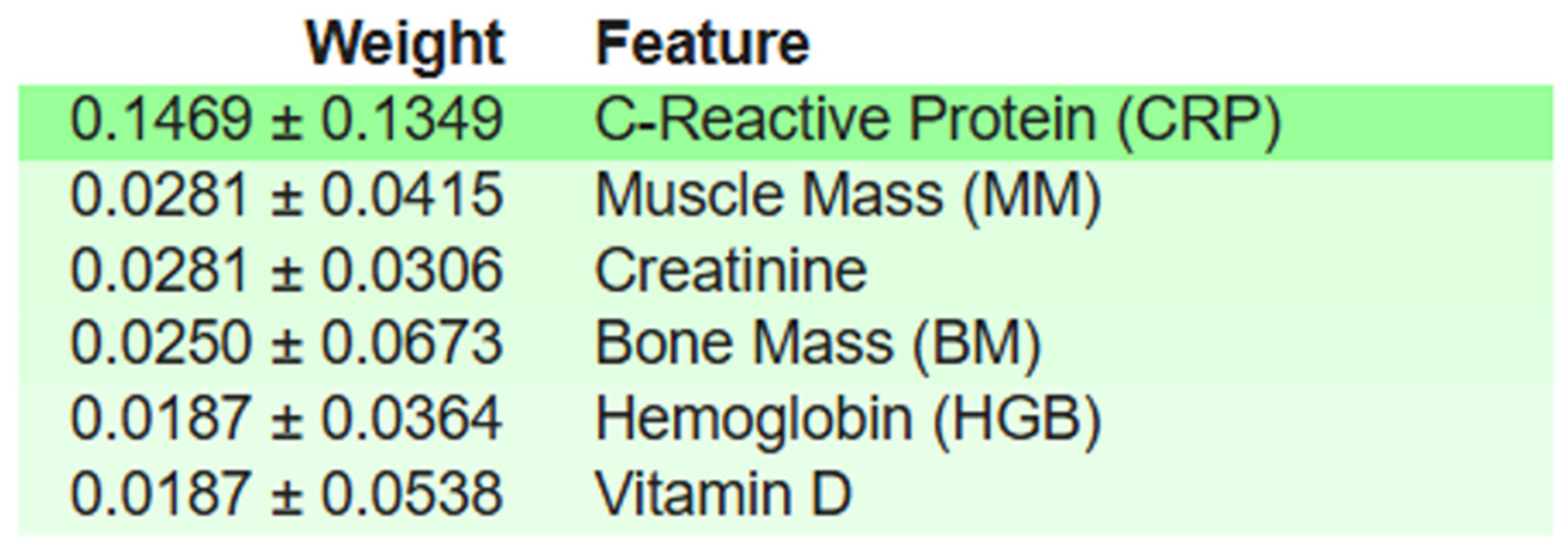
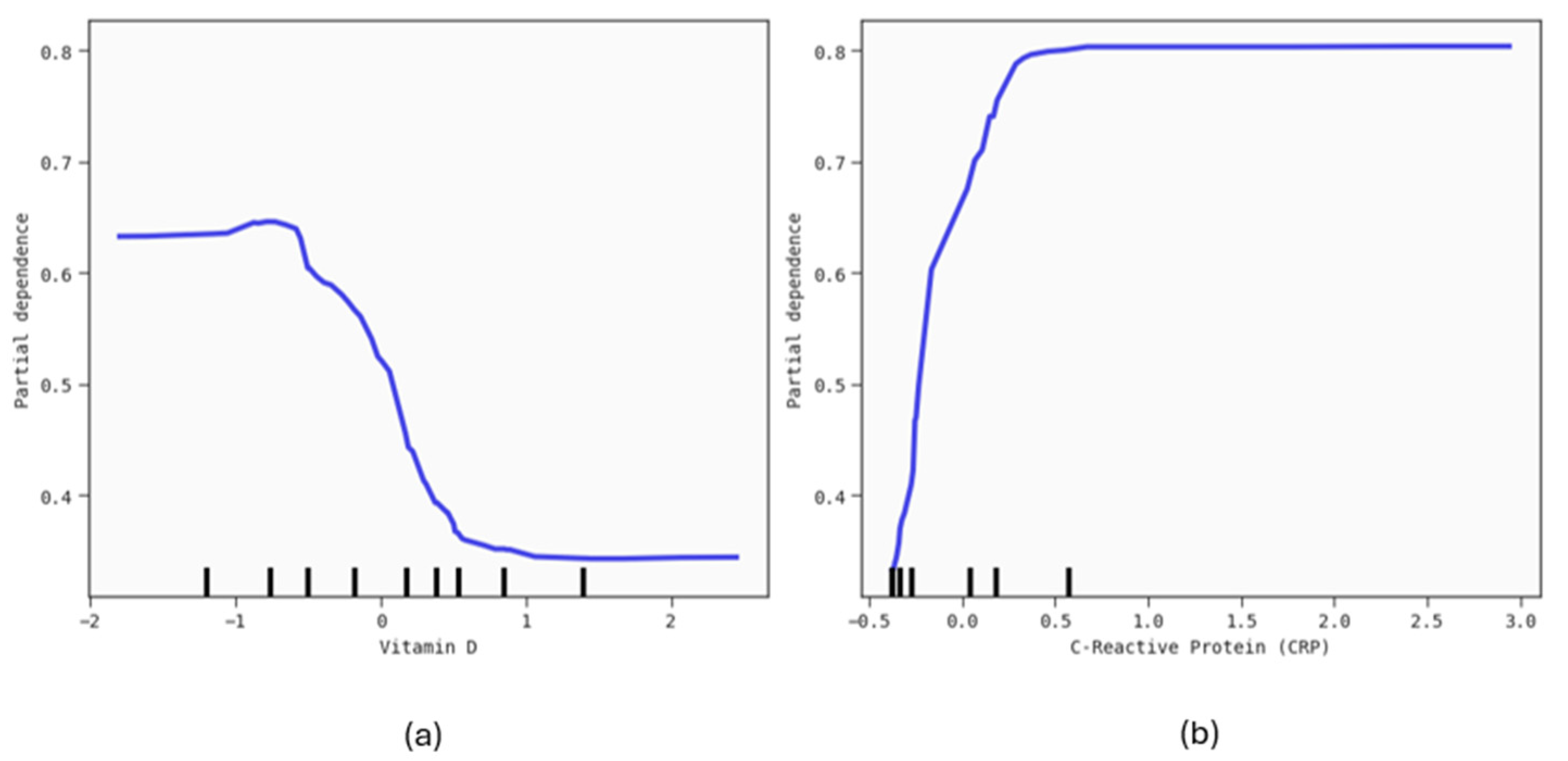
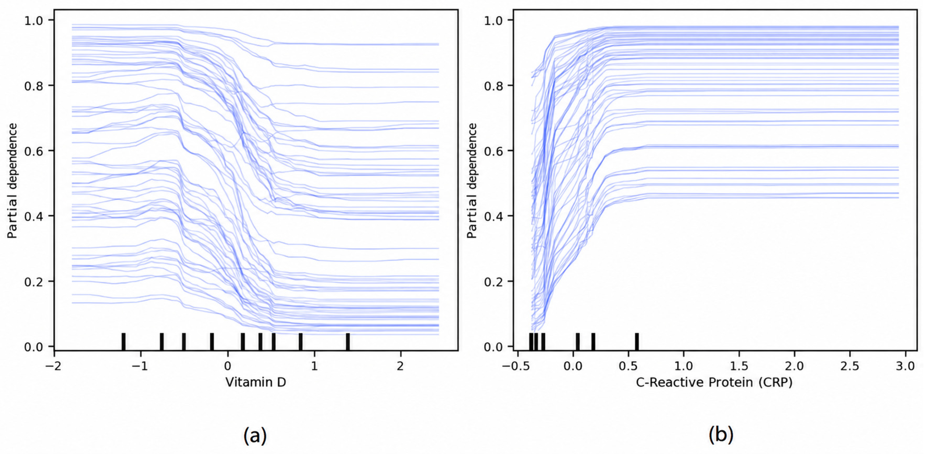
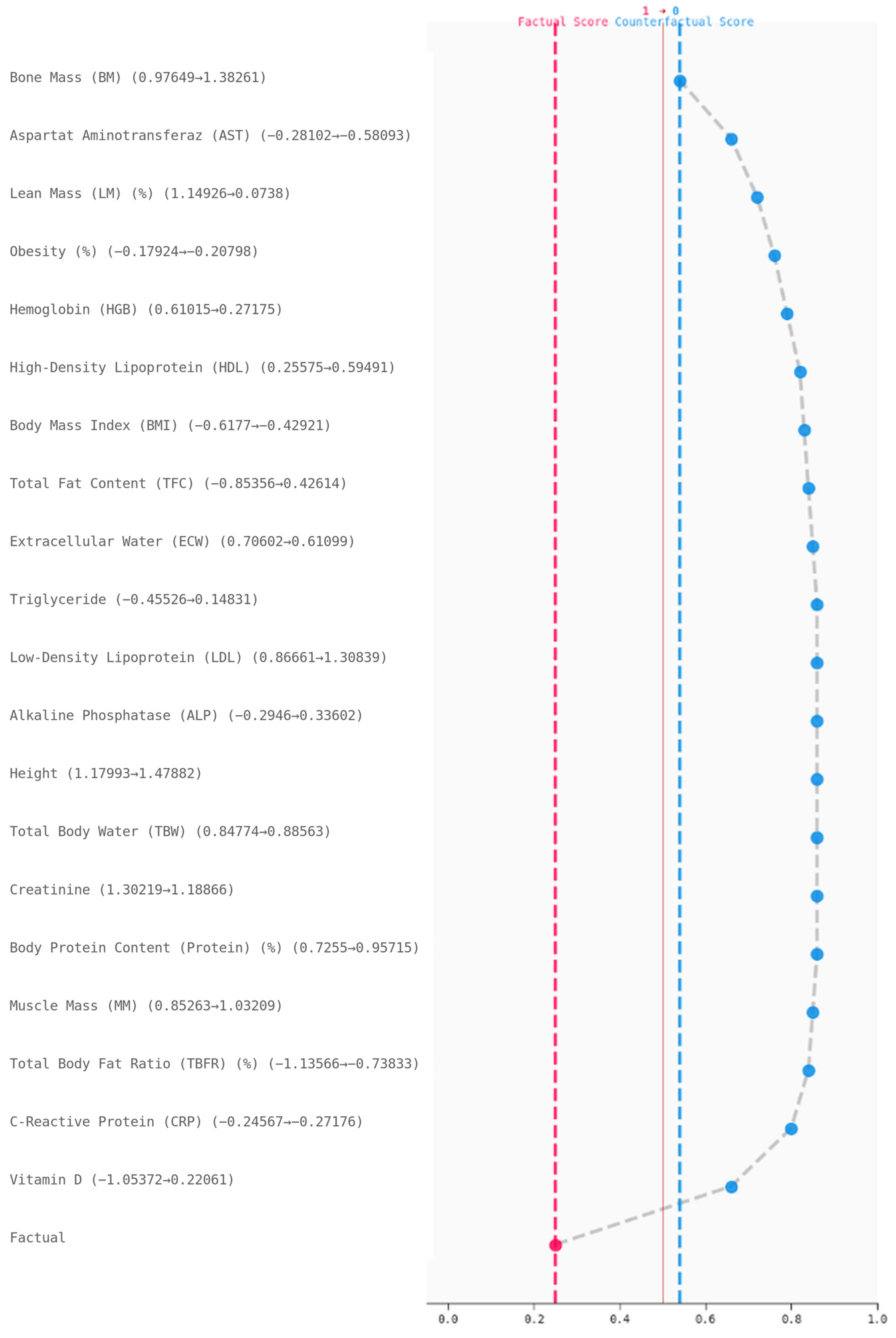
The predictions were explained using eight explainers. Further analysis was done using the stacking model with the randomized search technique since it obtained good results and combines multiple classifiers compared to individual baseline models. Figure 7 illustrates the SHAP beeswarm plot. The markers are organized in descending order of their significance. Hence, C-Reactive Protein (CRP), Vitamin D, obesity and Aspartate Aminotransferase (AST) were the attributes of high importance in predicting gallstone disease. Further, the two classes are divided by a vertical plane. The colors represent the value intensity, with blue showing lower values and red showing higher values. A higher muscle mass (MM) value decreases the chances of being predicted with gallstones. Figure 8 is a depiction of a force plot. A force plot is useful in interpreting the prediction made for each patient. Figure 9 depicts the SHAP waterfall plot for an individual case. It illustrates that Vitamin D, obesity, Aspartate Aminotransferase (AST) and muscle mass (MM) are associated with a higher model-predicted probability of gallstone presence, while Body Protein Content, High-Density Lipoprotein (HDL) and Extracellular Water (ECW) lower the model output for this individual case. The contradicting association of MM with gallstone formation is due to the difference between global interpretability (Figure 7) and local interpretability (Figure 9). MM shows a negative association with gallstones across the entire dataset. However, the waterfall plot in Figure 9 represents an individual case where the patient’s unique combination of features caused the model to weigh MM as the risk-increasing factor for that instance only. The beeswarm plot, force plot and waterfall plot were generated using the SHAP explainer. The LIME prediction for a gallstone-diseased patient is made in Figure 10. The LIME explainer arranges the parameters based on their importance. Attributes like Vitamin D, obesity and muscle mass are significant factors in indicating the presence of gallstones. Figure 11 consists of the details of interpretations made by Eli5. The most important markers were C-Reactive Protein (CRP) and muscle mass (MM). The QGraph generated by the QLattice model is illustrated in Figure 12. It can be inferred that C-Reactive Protein (CRP) and Vitamin D were the best markers. QLattice is an independently trained model. It uses symbolic regression to search over a space of mathematical expressions to find a simple interpretable equation that predicts the target directly from the data. In this research, the QLattice model utilized the “addition” activation function. PDP and ICE analyses were conducted on a preselected subset of top-ranked features identified via SHAP (Vitamin D and C-Reactive Protein). These plots illustrate the stacking ensemble’s behavior with respect to these specific markers and should not be interpreted as an independent or exhaustive assessment of feature importance across the full feature set. Figure 13 depicts the Partial Dependence Plot (PDP) for Vitamin D and C-Reactive Protein (CRP). The PDP for Vitamin D illustrates that lower Vitamin D levels are associated with a higher predicted outcome, and higher levels with a lower predicted outcome. From the PDP for CRP, it can be inferred that higher CRP levels are strongly associated with a higher predicted outcome. This feature appears to have a strong proportionality with the predicted outcome once it crosses a certain threshold. Figure 14 depicts the Individual Conditional Expectation (ICE) plot for Vitamin D and C-Reactive Protein (CRP). CRP shows a highly homogeneous and strong positive association on the predicted outcome. Higher CRP values are associated with a higher model-predicted probability of gallstone presence for almost every individual. Vitamin D shows a relatively homogeneous decreasing association. This means that lower Vitamin D values were generally associated with higher model-predicted probabilities. The anchor explainer identified C-Reactive Protein (CRP) and Vitamin D as important markers. The results of the anchor explainer are tabulated in Table 8. From Figure 15, a greedy chart for counterfactual explanations, it can be inferred that Vitamin D is influential in the prediction of gallstones.
Eight XAI techniques have been utilized in this study and according to them, the crucial parameters are Vitamin D and C-Reactive Protein (CRP). These markers can be used to predict gallstone disease. Table 9 is a tabulation of important markers according to the explainers. These provide deeper visual and rule-based interpretations. C-Reactive Protein and Vitamin D were found to be important across local (LIME, SHAP force plot), global (SHAP beeswarm, PDP, ICE), rule-based (anchor), and counterfactual (greedy counterfactual chart) methods. Table 10 shows the configuration of the eight XAI techniques used in this study.

4. Discussion

Multiple classifiers were used in this study to predict gallstones in patients. Three hyperparameter tuning techniques were used. The stacking model through the randomized search CV (cross-validation) technique achieved an F1-score of 84%, an accuracy of 83% and an AUC of 0.90. It was chosen over the CatBoost classifier and voting techniques as it provided optimal discrimination, generalization stability, and smooth probability estimates for XAI applications and clinical decision support system requirements.
The difference in the performance of the stacking model and baseline model highlights the limited classifying ability when solely relying on traditional clinical parameters associated with cholelithiasis. The ensemble model’s better performance can be attributed to the incorporation of additional features including Vitamin D and CRP. This may help in increasing the predictive accuracy of the model. A total of eight XAI techniques were utilized to identify the important markers.
C-Reactive Protein (CRP) and Vitamin D were identified as key parameters in predicting gallstones by the model. However, these are non-specific markers that are associated with many medical conditions. SHAP and LIME techniques have also identified obesity and muscle mass (MM) as crucial parameters affecting gallstone formation. These parameters were found to be important on feature importance rankings too. Although obesity did not reach univariate significance in the analysis (Mann–Whitney U, p = 0.864), it remained among the top-ranked features in the multivariable SHAP analysis. This is not a contradiction. Univariate testing measures a marginal group difference in isolation, while SHAP-based importance reflects a feature’s contribution within the full multivariable model, accounting for interactions with other markers.
The findings suggest gallstones are associated with low Vitamin D [27]. Another study by C. Bin et al. [28] has also found a positive association between Vitamin D and gallstone formation. This study too revealed that lower Vitamin D levels were associated with a higher model-predicted probability of gallstone presence in this dataset. Low Vitamin D might contribute to gallstone risk through several overlapping mechanisms. Vitamin D receptors (VDRs) are expressed in hepatocytes and biliary epithelium. Vitamin D signaling modulates bile acid synthesis and transport, lipid metabolism, and inflammatory tone. Vitamin D deficiency is associated with dyslipidemia, insulin resistance, and visceral adiposity. These are the states that promote cholesterol supersaturation of bile and reduce gallbladder motility, facilitating nucleation and stone growth. Vitamin D also influences smooth muscle function and may indirectly affect gallbladder emptying, with deficiency potentially impairing cholecystokinin-mediated contraction. These pathways provide biological reasoning for the observed inverse association between Vitamin D levels and gallstone predictions in our model. Elevated levels of CRP generally indicate inflammation. But CRP has been linked to gallstone formation in prior studies and higher CRP levels imply greater chances of finding gallstones [29]. This study also highlighted that higher CRP levels were associated with a higher model-predicted probability of gallstone presence. The beeswarm plot suggested that higher MM was associated with lesser chances of gallstone formation, while the waterfall plot listed MM as a parameter that increased the prediction in a specific case. Hence, it can be concluded that MM is a potentially unstable predictor whose effect may be sample-specific or interaction-dependent. However, there are various studies that testify the association between low muscle mass and the formation of gallstones [30].
Table 11 consists of the comparison of the proposed model with similar research. This is the first research that uses eight Explainable Artificial Intelligence (XAI) techniques to predict gallstones.
Vitamin D was identified as important by all eight XAI methods applied in this study, while CRP was identified by six of eight, consistent with Table 9. However, because these explainers are applied to the same model, the same 319-patient dataset, and a partially correlated feature set, this cross-method agreement reflects consistent model behavior rather than independent statistical or biological validation.
It is worth noting that SHAP and LIME are known to be sensitive to feature collinearity, particularly on small tabular biomedical datasets. Several markers in this dataset are correlated with one another. Body Mass Index, for instance, is moderately to strongly correlated with Extracellular Water and Total Body Water. Attribution among these body composition markers should therefore be read as importance distributed across a correlated cluster, rather than as independent contributions from each variable. C-Reactive Protein showed weak correlation with the other markers examined, so its attribution is less likely to be affected by this issue.
On the contrary, MM was highlighted only by two explainers. This inconsistency implies that MM’s contribution is conditional, unstable and likely dependent on interactions with adiposity or inflammatory markers. It was found that lower Body Protein Content, HDL, and ECW were associated with a higher model-predicted probability of gallstone presence in this dataset. As this is a cross-sectional, associative analysis, these findings should not be interpreted as evidence that dietary protein intake or supplementation prevents cholelithiasis.
The implementation of XAI techniques improves the clinical applicability of ML models. They also help in understanding how certain markers are influential in predicting gallstones. XAI techniques facilitate model validation by revealing potential biases or errors in the prediction logic, ensuring the model’s fairness and robustness across different patient groups.
There are certain limitations in this research. The dataset used for this research consisted of the data from 319 individuals, where 161 were diagnosed with gallstones. This increases the risk of overfitting and limits the generalizability of the model. External validation was not performed. This limits the clinical utility of the model. With 38 correlated predictors and 319 samples, evaluating nine base learners under three tuning strategies and two ensembling schemes carries meaningful risk of model selection bias. The cross-validation and reported confidence intervals partially mitigate but do not fully eliminate this risk. Multiple-testing correction was not applied to the univariate comparisons. This raises the possibility that some markers reaching statistical significance do so by chance rather than reflecting a true group difference. This risk is limited to the univariate screening analysis and does not affect the machine learning models, whose feature importance is derived from the Fisher’s score. The reliance of the model on non-specific parameters introduces the risk of false positive cases. Patients with inflammatory conditions and Vitamin D deficiency may be falsely classified as having cholelithiasis. Moreover, measuring CRP and Vitamin D is not clinically feasible as a first step in diagnosis. Therefore, this proposed model at present can be used only as a tool in assisting gallstone diagnosis. These limitations highlight the fact that ultrasound imaging would still remain as the diagnostic tool for gallstones. Additionally, the diagnostic reference standard used to establish gallstone status in the original data source is not specified. This limits our ability to assess potential diagnostic misclassification.
ML models will evolve to capture complex patterns and subtle risk factors that traditional methods might overlook once larger datasets are available. By using deep learning (DL) techniques on ultrasound images, such predictions could be made even more accurately [31]. The integration of ML and XAI paves the way for more accurate diagnosis of gallstone disease. XAI techniques enhance the interpretability of the model. They will play a crucial role in ensuring that these models remain transparent and clinically interpretable. The future research must include multi-centric data collection to make the model generalizable and more reliable. Validation of the model with external data is crucial to increase the reliability of the model. The scope of this study may be reframed towards identifying potential risk factors for gallstone formation. This would enhance the contribution of the study by aligning it with preventive medicine and public health goals. Additionally, deploying cloud-based systems can enhance the accessibility and security of the data.

5. Conclusions

Various machine learning algorithms and Explainable Artificial Intelligence techniques were utilized in this research, to predict gallstones based on clinical parameters. The eight XAI techniques, namely, SHAP, LIME, Eli5, QLattice, PDP, ICE, anchor and counterfactual explanations were also utilized to interpret the outcomes. These increased the interpretability and explainability of the model. Understanding the reasoning behind the prediction is as crucial as the prognosis. An F1-score of 84%, an accuracy of 83% and an AUC of 0.90 were obtained by the customized ensemble model. Vitamin D, C-Reactive Protein, obesity and muscle mass were identified as the crucial markers in predicting gallstones. The model captures the physical and physiological markers associated with gallstone presence in this dataset. These results indicate that ML models can be effectively incorporated into clinical decision support systems to assist medical professionals in risk categorization, facilitating timely clinical discussion between patients and providers. ML and XAI have the potential to improve and expand the realm of gallstone prediction. Integrating digital health records, medical imaging, and genomics is a key strategy. Combining these data sources can make the predictive model more reliable. Therefore, these measures would help in achieving preventive medicine and public health goals of ensuring good health and well-being.
Apart from increasing the accuracy of the decision-making process, the suggested tool will increase the accountability of the human decision-maker, a feature becoming increasingly important when designing tools for the clinical application of artificial intelligence. The model is not supposed to act as a completely independent diagnostic tool but works under a human-in-the-loop approach, where the clinician is ultimately responsible for the diagnostic decision and the XAI techniques assist in that decision. The SHAP and LIME techniques give us an estimate of the impact of each clinical marker on prediction in one particular patient, thus giving an opportunity for the clinician to check if the reasoning of the model for the patient is biologically plausible or not. PDPs, ICEs, and QLattice illustrate how markers such as Vitamin D and CRP relate to the model’s predicted probability of gallstone presence, and the clinician will be able to confirm that the model behaves in a realistic manner. The anchor explanations provide rule-based justifications for the model prediction. The counterfactual explanations give the clinician the information about the smallest change in a patient’s characteristics necessary to change the prediction. Thus, the clinician may use this information to explain the decision to the patient and justify it retrospectively. In addition, since all predictions of the model can be tracked down to the specific combination of markers that could be understood by humans, the clinician is not required to trust the output of the model blindly but can critically evaluate it and either agree or disapprove. This shifts the locus of accountability back to the clinician, who remains the responsible decision-maker, with the model serving as an auditable aid rather than a black box replacement.

Author Contributions

A.N.S.: Writing—original draft, visualization, software; K.C.: conceptualization, data curation, writing—review and editing; D.B.: writing—review and editing, resources, visualization; N.S.: supervision, formal analysis, validation. All authors have read and agreed to the published version of the manuscript.

Funding

This research received no external funding.

Data Availability Statement

The data supporting the findings of this study includes external data. The dataset used in this study is openly available in the UCI Machine Learning Repository. https://archive.ics.uci.edu/dataset/1150/gallstone-1 (accessed on 9 June 2025).

Acknowledgments

The authors would like to thank the Manipal Academy of Higher Education for their support.

Conflicts of Interest

The authors declare no conflicts of interest.

Appendix A. Mathematical Formulations of the Machine Learning Algorithms and Hyperparameter Tuning Methods

This appendix documents the mathematical formulation of every algorithm used in this study, expressed in vector/matrix form. The feature matrix is denoted as X ∈ ℝn×p, where n is the number of samples and p the number of clinical markers. An individual sample is the row vector xi ∈ ℝp, and a new input for prediction is x. The true label vector is y ∈ {0,1}n. Model parameters include a weight vector w ∈ ℝp and scalar bias b. Predicted probabilities/labels are denoted as ŷ.

Appendix A.1. Logistic Regression

1. Mathematical Formulation
The linear combination of features is passed through the sigmoid function σ(z) = 1/(1 + e−z):
z = Xw + b1 ŷ = σ(z)
where 1 is a vector of ones broadcasting the bias across all n samples.
2. Training Objective
Binary cross-entropy loss with L2 regularization:
L(w, b) = −(1/n)Σi=1n [yi log ŷi + (1−yi) log(1−ŷi)] + λ‖w‖2
3. Prediction Rule
ŷ = 1 if σ(xw + b) ≥ 0.5, else 0
4. Operation Type
A direct matrix–vector multiplication (Xw) followed by scalar addition and element-wise sigmoid activation—a purely linear model.

Appendix A.2. K-Nearest Neighbors (KNNs)

1. Mathematical Formulation
The vectorized squared Euclidean distance matrix between the test and train samples:
D2 = ‖Xtest‖21T − 2XtestXtrainT + 1‖Xtrain‖2
so that D2ij = ‖xtest,i − xtrain,j‖2, computed for all pairs at once rather than one at a time.
2. Training Objective
KNN is instance-based: the training data is stored, and no explicit loss function is minimized during training.
3. Prediction Rule
Let Nk(x) be the k nearest training vectors to x. The predicted label is the majority class among them:
ŷ = argmaxc∈{0,1} Σxjj∈Nk(x) 1(yj = c)
4. Operation Type
A distance-based computation: prediction depends on the pairwise distance of the query to every training vector, not on a single matrix–vector product.

Appendix A.3. Support Vector Machine (SVM)

Appendix A.3.1. Linear SVM

1. Mathematical Formulation
f(xi) = xiw + b, with labels yi ∈ {−1, +1}
2. Training Objective
Hinge loss with L2 regularization, maximizing the margin between classes:
L(w, b) = (1/n) Σi=1n max(0, 1 − yif(xi)) + λ‖w‖2
3. Prediction Rule
ŷ = sgn(xw + b)
4. Operation Type
A direct matrix–vector multiplication for linear separation of classes.

Appendix A.3.2. Kernel SVM (RBF Kernel)

1. Mathematical Formulation
With support vectors xsvi, dual coefficients αi, and RBF kernel K(xa,xb) = exp(−γ‖xa − xb‖2):
f(x) = Σi∈SV αiysviK(x, xsvi) + b
2. Training Objective
Maximize the dual objective, subject to box constraints on α:
L(α) = Σi=1n αi − (1/2) Σi,j αiαjyiyjK(xi, xj)
subject to 0 ≤ αi ≤ C and Σiyiαi = 0.
3. Prediction Rule
ŷ = sgn(Σi∈SV αiysviK(x, xsvi) + b)
4. Operation Type
A kernel/distance-based computation—the RBF kernel itself is a function of the distance between vectors.

Appendix A.4. Decision Tree Classifier

1. Mathematical Formulation
The feature space is partitioned into M rectangular regions Rm; a sample in region Rm receives constant prediction cm:
h(x) = Σm=1M cm 1(x ∈ Rm)
2. Training Objective
Nodes are split recursively to minimize child node impurity (maximize information gain):
Gini: G(p) = Σk=1K pk(1−pk) Entropy: E(p) = −Σk=1K pk log2 pk
3. Prediction Rule
Traverse the tree from the root, evaluating one feature condition per internal node; predict the majority class of the leaf reached.
4. Operation Type
A rule-based/sequential computation—a series of conditional evaluations, not a single matrix operation.

Appendix A.5. Random Forest

1. Mathematical Formulation
An ensemble of B decorrelated trees hb, each trained on a bootstrap sample with a random feature subset:
H(x) = argmaxc∈{0,1} Σb=1B 1(hb(x) = c)
2. Training Objective
Each tree minimizes impurity as in Appendix A.4; averaging diverse trees reduces variance and improves generalization.
3. Prediction Rule
ŷ = argmaxc∈{0,1} Σb=1B 1(ŷb = c)
4. Operation Type
Aggregation of sub-models—many decorrelated trees combined by majority vote.

Appendix A.6. AdaBoost

1. Mathematical Formulation
M weak learners hm(x), each weighted by αm, with labels and predictions in {−1, +1}:
H(x) = sgn(Σm=1M αmhm(x))
2. Training Objective
Minimizes exponential loss by iteratively training weak learners on reweighted samples:
L = Σi=1n exp(−yiH(xi)) αm = (1/2) ln((1−εm)/εm)
where εm is the weighted error of hm, and sample weights are updated as wi^(t + 1) ∝ wi^(t) exp(−αm yi hm(xi)).
3. Prediction Rule
ŷ = sgn(Σm=1M αmhm(x))
4. Operation Type
Aggregation of sub-models—sequentially trained weak learners focused on previously misclassified samples, combined by weighted vote.

Appendix A.7. Gradient Boosting

1. Mathematical Formulation
An additive model built by sequentially adding M trees hm with step sizes (learning rates) ρm:
FM(x) = Σm=1M ρmhm(x)
2. Training Objective
Each new tree is fit to the negative gradient (pseudo-residual) of the loss w.r.t. the current ensemble prediction:
rim = − [∂L(yi, F(xi))/∂F(xi)]F=Fm−1
3. Prediction Rule
ŷ = FM(x) = Σm=1M ρmhm(x)
4. Operation Type
Aggregation of sub-models—trees sequentially fit to correct prior residuals, combined additively.

Appendix A.8. XGBoost

1. Mathematical Formulation
FM(x) = Σm=1Mhm(x)
2. Training Objective
A regularized objective minimized via a second-order Taylor expansion of the loss at iteration t:
L(t) = Σi=1n [giht(xi) + (1/2) Hiht2(xi)] + Ω(ht)
with gi = ∂L/∂Ft−1, Hi = ∂2L/∂F2t−1, and Ω(ht) = γT + (1/2)λ‖w‖2 (T = number of leaves).
Optimal leaf weight:
w*j = − (Σi∈Ijgi)/(Σi∈IjHi + λ)
3. Prediction Rule
ŷ = FM(x) = Σm=1Mhm(x)
4. Operation Type
Aggregation of sub-models, as in gradient boosting, with an enhanced regularized objective using second-order gradients.

Appendix A.9. CatBoost

1. Mathematical Formulation
Also, an additive tree ensemble, but built using a permutation-driven (ordered) boosting scheme:
FM(x) = Σm=1Mhm(x)
2. Training Objective
Minimizes LogLoss as in standard gradient boosting, but each residual for sample i is estimated using a model trained only on samples preceding i in a random permutation (ordered boosting), reducing target leakage/prediction shift. Categorical features are encoded on-the-fly using permutation-based target statistics rather than static encodings.
3. Prediction Rule
ŷ = σ(FM(x)) = σ(Σm=1Mhm(x))
4. Operation Type
Aggregation of sub-models with sequential (ordered) training, adding native handling of categorical features and reduced prediction shift.

Appendix A.10. Customized Stacking Ensemble (Meta-Learner)

1. Mathematical Formulation
Predictions of the K = 9 base learners (Appendix A.1, Appendix A.2, Appendix A.3, Appendix A.4, Appendix A.5, Appendix A.6, Appendix A.7, Appendix A.8 and Appendix A.9) for input x form a meta-feature vector:
z = [h1(x), h2(x), …, hK(x)]
The meta-learner g (logistic regression) then predicts from this vector:
ŷ = g(z)
2. Training Objective
Two-stage training: (i) base learners are trained on the original data; (ii) out-of-fold predictions of the base learners form a new training set on which the meta-learner g is trained to minimize its own loss (binary cross-entropy).
3. Prediction Rule
ŷ = g(h1(x), …, hK(x))
4. Operation Type
A hierarchical aggregation of sub-models—a meta-learner learns to optimally combine the outputs of nine diverse base learners.

Appendix A.11. Hyperparameter Tuning Methods

Appendix A.11.1. Grid Search

For hyperparameters θ1,…,θP with candidate sets S1,…,SP, grid search exhaustively evaluates every combination (|S1|×…×|SP| total):
(θ*1,…,θ*P) = argmax(θ1,…,θP)∈S1×…SP PerformanceMetric(Model(θ1,…,θP))
Operation type: deterministic, exhaustive search over a discretized hyperparameter grid.

Appendix A.11.2. Randomized Search

Instead of exhaustive enumeration, N combinations are sampled from distributions De defined over each hyperparameter, θp,j~Dp, and the best-performing sampled combination is selected. This is markedly cheaper than grid search when many hyperparameters are uninformative.
Operation type: non-exhaustive, stochastic search over the hyperparameter space.

Appendix A.11.3. Bayesian Optimization

A sequential, model-based strategy for optimizing an expensive objective f (cross-validation performance). A surrogate model (Gaussian Process) P(f|D) is fit to prior observations D = {(θ1,y1),…,(θt,yt)}, and an acquisition function a(θ|D) (e.g., Expected Improvement) selects the next point to evaluate:
θt+1 = argmaxθ a(θ | D)
Operation type: sequential, model-based optimization balancing exploration and exploitation, rather than an exhaustive or purely random search.

References

  1. Sanders, G.; Kingsnorth, A.N. Gallstones. BMJ Clin. Rev. 2007, 335, 295–299. [Google Scholar] [CrossRef] [Scilit]
  2. Lammert, F.; Gurusamy, K.; Ko, C.W.; Miquel, J.-F.; Méndez-Sánchez, N.; Portincasa, P.; van Erpecum, K.J.; van Laarhoven, C.J.; Wang, D.Q.-H. Gallstones. Nat. Rev. Dis. Primers 2016, 2, 16024. [Google Scholar] [PubMed]
  3. Johnston, D.E.; Kaplan, M.M. Pathogenesis and Treatment of Gallstones. N. Engl. J. Med. 1993, 328, 412–421. [Google Scholar] [CrossRef] [Scilit] [PubMed]
  4. Gaby, A.R. Nutritional approaches to prevention and treatment of gallstones. Altern. Med. Rev. 2009, 14, 258. [Google Scholar] [PubMed]
  5. Friedman, M.G.D. Natural history of asymptomatic and symptomatic gallstones. Am. J. Surg. 1993, 165, 399–404. [Google Scholar] [CrossRef] [Scilit] [PubMed]
  6. Deng, L.; Wang, S.; Wan, D.; Zhang, Q.; Shen, W.; Liu, X.; Zhang, Y. Relative Fat Mass and Physical Indices as Predictors of Gallstone Formation: Insights from Machine Learning and Logistic Regression. Int. J. Gen. Med. 2025, 18, 509–527. [Google Scholar] [CrossRef] [Scilit] [PubMed]
  7. Ma, Y.; Yue, P.; Zhang, J.; Yuan, J.; Liu, Z.; Chen, Z. Early prediction of acute gallstone pancreatitis. Ann. Med. 2024, 56, 2357354. [Google Scholar] [CrossRef] [Scilit] [PubMed]
  8. Salem, N.M.; Jack, K.M.; Gu, H.; Kumar, A.; Garcia, M.; Yang, P.; Dinu, V. Machine and deep learning identified metabolites and clinical features. Comput. Methods Programs Biomed. Update 2023, 3, 100106. [Google Scholar] [CrossRef] [Scilit]
  9. Esen, İ.; Arslan, H.; Aktürk Esen, S.M.; Gülşen, M.; Kültekin, N.; Özdemir, O.M. Early prediction of gallstone disease with a machine learning-based method from bioimpedance and laboratory data. Medicine 2024, 103, 8. [Google Scholar] [CrossRef] [Scilit] [PubMed]
  10. Hong, C.; Zafar, I.; Ayaz, M.M.; Kanwal, R.; Kanwal, F.; Dauelbait, M.; Bourhia, M.; Jardan, Y.A.B. Analysis of Machine Learning Algorithms for Real-Time Gallbladder Stone Identification from Ultrasound Images in Clinical Decision Support Systems. Int. J. Comput. Intell. Syst. 2025, 18, 73. [Google Scholar] [CrossRef] [Scilit]
  11. Dalai, C.; Azizian, J.M.; Trieu, H.; Rajan, A.; Chen, F.; Dong, T.; Beaven, S.W.; Tabibian, J.H. Machine learning models compared to existing criteria for noninvasive prediction of endoscopic retrograde cholangiopancreatography-confirmed choledocholithiasis. Liver Res. 2021, 5, 224–231. [Google Scholar] [CrossRef] [Scilit] [PubMed]
  12. Zhang, X.; Yue, P.; Zhang, J.; Yang, M.; Chen, J.; Zhang, B.; Luo, W.; Wang, M.; Da, Z.; Li, X.; et al. A novel machine learning model and a public online prediction platform for prediction of post-ERCP-cholecystitis (PEC). eClinicalMedicine 2022, 48, 101431. [Google Scholar] [CrossRef] [Scilit] [PubMed]
  13. Shao, G.; Ma, Y.; Wang, L.; Qu, C.; Gao, R.; Sun, P.; Cao, J. Machine learning models based on dietary data to predict gallstones: NHANES 2017–2020. Res. Sq. 2024. [Google Scholar] [CrossRef] [Scilit] [PubMed]
  14. Ahsan, M.M.; Mahmud, M.A.P.; Saha, P.K.; Gupta, K.D.; Siddique, Z. Effect of Data Scaling Methods on Machine Learning Algorithms and Model Performance. Technologies 2021, 9, 52. [Google Scholar] [CrossRef] [Scilit]
  15. Koopialipoor, M.; Asteris, P.G.; Mohammed, A.S.; Alexakis, D.E.; Mamou, A.; Armaghani, D.J. Introducing stacking machine learning approaches for the prediction of rock deformation. Transp. Geotech. 2022, 34, 100756. [Google Scholar] [CrossRef] [Scilit]
  16. Feng, D.-C.; Wang, W.-J.; Mangalathu, S.; Taciroglu, E. Interpretable XGBoost-SHAP Machine-Learning Model for Shear Strength Prediction of Squat RC Walls. J. Struct. Eng. 2021, 147, 04021173. [Google Scholar] [CrossRef] [Scilit]
  17. Garreau, D.; von Luxburg, U. Explaining the Explainer: A First Theoretical Analysis of LIME. In Proceedings of the Twenty Third International Conference on Artificial Intelligence and Statistics, Palermo, Italy, 26–28 August 2020; Volume 108, pp. 1287–1296. [Google Scholar]
  18. Kerrigan, D.; Barr, B.; Bertini, E. PDPilot: Exploring Partial Dependence Plots Through Ranking, Filtering, and Clustering. IEEE Trans. Vis. Comput. Graph. 2025, 3, 7377–7390. [Google Scholar] [CrossRef] [Scilit] [PubMed]
  19. Sun, D.; Ding, Y.; Wen, H.; Zhang, F. A novel QLattice-based whitening machine learning model of landslide susceptibility mapping. Earth Surf. Processes Landf. 2023, 49, 304–317. [Google Scholar] [CrossRef] [Scilit]
  20. Goldstein, A.; Kapelner, A.; Bleich, J.; Pitkin, E. Peeking Inside the Black Box: Visualizing Statistical Learning with Plots of Individual Conditional Expectation. J. Comput. Graph. Stat. 2015, 24, 44–65. [Google Scholar] [CrossRef] [Scilit]
  21. Khanna, V.V.; Chadaga, K.; Sampathila, N.; Prabhu, S. A machine learning and explainable artificial intelligence triage-prediction system for COVID-19. Decis. Anal. J. 2023, 7, 100246. [Google Scholar] [CrossRef] [Scilit]
  22. Thanathamathee, P.; Sawangarreerak, S.; Nizam, D.N.M. Enhancing Going Concern Prediction with Anchor Explainable AI and Attention-Weighted XGBoost. IEEE Access 2024, 12, 68345–68363. [Google Scholar] [CrossRef] [Scilit]
  23. Guidotti, R. Counterfactual explanations and how to find them: Literature review and benchmarking. Data Min. Knowl. Discov. 2022, 38, 2770–2824. [Google Scholar] [CrossRef] [Scilit]
  24. Belete, D.M.; Huchaiah, M.D. Grid search in hyperparameter optimization of machine learning models for prediction of HIV/AIDS test results. Int. J. Comput. Appl. 2022, 44, 875–886. [Google Scholar] [CrossRef] [Scilit]
  25. Subaşı, N. Comprehensive Analysis of Grid and Randomized Search on Dataset Performance. Eur. J. Eng. Appl. Sci. 2024, 7, 77–83. [Google Scholar] [CrossRef] [Scilit]
  26. Stuke, A.; Rinke, P.; Todorović, M. Efficient hyperparameter tuning for kernel ridge regression with bayesian optimization. Mach. Learn. Sci. Technol. 2021, 2, 035022. [Google Scholar] [CrossRef] [Scilit]
  27. Kumar, D.; Mehta, M.A.; Kotecha, K.; Kulkarni, A. Computer-aided cholelithiasis diagnosis using explainable convolutional neural network. Sci. Rep. 2025, 15, 4249. [Google Scholar] [CrossRef] [Scilit] [PubMed]
  28. Bin, C.; Zhang, C. The association between vitamin D consumption and gallstones in US adults: A cross-sectional study from the national health and nutrition examination survey. J. Formos. Med. Assoc. 2025, 124, 212–217. [Google Scholar] [CrossRef] [Scilit] [PubMed]
  29. Jiang, Z.; Jiang, H.; Zhu, X.; Zhao, D.; Su, F. The relationship between high-sensitivity C-reactive protein and gallstones: A cross-sectional analysis. Front. Med. 2024, 11, 1453129. [Google Scholar] [CrossRef] [Scilit] [PubMed]
  30. Ataş, A.E.; Ünüvar, Ş. High visceral adiposity and low skeletal muscle mass independently predict the development of acute cholecystitis in patients with gallstones: A retrospective cohort study. Front. Med. 2025, 12, 1724416. [Google Scholar] [CrossRef] [Scilit] [PubMed]
  31. Ali, M.L.; Zhang, Z. The YOLO Framework: A Comprehensive Review of Evolution, Applications, and Benchmarks in Object Detection. Computers 2024, 13, 336. [Google Scholar] [CrossRef] [Scilit]
Figure 1. The common symptoms, causes and treatments for gallstones.
Computers 15 00668 g001
Figure 2. Feature importance based on Fisher’s score.
Computers 15 00668 g002
Figure 3. Violin plots that depict marker variation. (a) Extracellular Water, (b) Vitamin D, (c) Visceral Muscle Area, (d) Hemoglobin.
Computers 15 00668 g003
Figure 4. Receiver Operating Characteristic (ROC) curves for the final stacking model. (a) Grid search, (b) randomized search, (c) Bayesian optimization algorithm.
Computers 15 00668 g004
Figure 5. Precision–recall (PR) curves for the final stacking model. (a) Grid search, (b) randomized search, (c) Bayesian optimization algorithm.
Computers 15 00668 g005
Figure 6. Confusion matrix for the final stacking model. (a) Grid search, (b) randomized search, (c) Bayesian optimization algorithm.
Computers 15 00668 g006
Figure 7. SHAP beeswarm plot to decipher gallstone prediction. All 38 features were used for model training; features beyond the top 20 are omitted here for readability.
Computers 15 00668 g007
Figure 8. SHAP force plot for an individual with gallstones.
Computers 15 00668 g008
Figure 9. SHAP waterfall plot for an individual with gallstones.
Computers 15 00668 g009
Figure 10. LIME model to decipher gallstone positive predictions.
Computers 15 00668 g010
Figure 11. Eli5 technique to understand crucial parameters in gallstone prediction.
Computers 15 00668 g011
Figure 12. QGraph, ROC curve and confusion matrix of QLattice model to understand significant markers in gallstone prediction.
Computers 15 00668 g012
Figure 13. Partial Dependent Plot (PDP) for (a) Vitamin D, (b) C-Reactive Protein.
Computers 15 00668 g013
Figure 14. Individual Conditional Expectation (ICE) for (a) Vitamin D, (b) C-Reactive Protein.
Computers 15 00668 g014
Figure 15. Greedy chart for counterfactual explanation.
Computers 15 00668 g015
Table 1. Tabulation of research findings by various authors.
AuthorsData UsedML ModelsAccuracyXAI Techniques
Chen Hong et al. [10]Local hospitalsRandom Forest96.33%Grad-CAM, saliency maps
C. Dalai et al. [11]ERCP-confirmed patient dataXGBoost, RF, SVM83%SHAP
Xu Zhang et al. [12]ERCP patient recordsLogistic regression, XGBoost85.5%SHAP
Guanming Shao et al. [13]NHANES (2017–2020)XGBoost88%SHAP
Table 2. Markers used to predict the presence of gallstone disease.
MarkerDescriptionMarkerDescription
1. AgeAge of the person20. Muscle mass (MM)Muscle weight
2. GenderGender of the person21. ObesityExcessive adiposity
3. ComorbidityConcomitant diseases22. Total fat content (TFC)Total fat amount
4. Coronary Artery Disease (CAD)Cardiovascular disease23. Visceral Fat Area (VFA)Inner adipose tissue area
5. HypothyroidismUnderactive thyroid gland24. Visceral Muscle Area (VMA)Inner muscle area
6. HyperlipidemiaHigh levels of fat in the blood25. Hepatic Fat Accumulation (HFA)Accumulation of fat in the liver
7. Diabetes Mellitus (DM)High blood sugar26. GlucoseBlood sugar
8. HeightHeight is the length27. Total cholesterol (TC)It is total cholesterol
9. WeightBody weight28. Low-Density Lipoprotein (LDL)Bad cholesterol
10. Body Mass Index (BMI)Weight for height ratio29. High-Density Lipoprotein (HDL)Good cholesterol
11. Total Body Water (TBW)Total water in the body30. TriglycerideType of fat found in the blood
12. Extracellular water (ECW)It is extracellular water31. Aspartate Aminotransferase (AST)Type of liver enzyme
13. Intracellular water (ICW)It is intracellular water32. Alanine Aminotransferase (ALT)An enzyme related to the liver
14. Extracellular Fluid/Total Body Water (ECF/TBW)Extracellular water content33. Alkaline Phosphatase (ALP)Type of liver and bone enzyme
15. Total Body Fat Ratio (TBFR)Total fat content34. CreatinineKidney function indicator
16. Lean Mass (LM)Lean body mass35. Glomerular Filtration Rate (GFR)Kidney filtration rate
17. Body Protein Content (Protein)Essential building blocks for the body36. C-Reactive Protein (CRP)Inflammation indicator
18. Visceral Fat Rating (VFR)Visceral organ fat level37. Hemoglobin (HGB)Protein in the blood that carries oxygen
19. Bone Mass (BM)Bone weight38. Vitamin DEssential vitamin for bone health
Table 3. Descriptive statistical measures for continuous attributes.
DiagnosisMeanMedianStandard DeviationPercentiles
25th50th75th
AgeGallstone47.63449.00012.97038.00049.00056.000
No Gallstone48.51350.00011.20039.25050.00056.000
HeightGallstone168.230170.0009.772162.000170.000175.000
No Gallstone166.063165.00010.247158.000165.000174.000
WeightGallstone79.80978.00015.97669.20078.00090.500
No Gallstone81.33579.85015.44570.22579.85092.150
Body Mass
Index (BMI)
Gallstone28.23927.7005.29124.80027.70031.400
No Gallstone29.52829.1505.27526.02529.15032.475
Total Body
Water (TBW)
Gallstone41.46041.6007.81435.00041.60047.100
No Gallstone39.69938.2507.97433.62538.25046.600
Extracellular
Water (ECW)
Gallstone17.62917.5002.94315.70017.50019.700
No Gallstone16.50316.5503.28314.00016.55018.975
Intracellular
Water (ICW)
Gallstone23.82123.6005.10419.20023.60027.500
No Gallstone23.44422.5505.59819.52522.55027.950
Extracellular
Fluid/Total Body Water
(ECF/TBW)
Gallstone42.75742.0002.77841.00042.00044.000
No Gallstone41.65742.0003.58439.82042.00044.000
Total Body Fat
Ratio (TBFR) (%)
Gallstone26.39225.8008.40820.10025.80031.700
No Gallstone30.19431.0508.06523.99231.05036.015
Lean Mass (LM)
(%)
Gallstone73.52273.9308.38468.32073.93079.750
No Gallstone69.71868.7908.07563.99268.79075.995
Body Protein
Content
(Protein) (%)
Gallstone16.13816.1302.10214.67016.13017.420
No Gallstone15.73515.6102.54114.20015.61017.408
Bone Mass (BM)Gallstone2.9122.9000.4972.5002.9003.300
No Gallstone2.6922.6000.5002.3002.6003.000
Muscle Mass
(MM)
Gallstone55.25255.20010.14046.50055.20063.000
No Gallstone53.27652.25010.99944.75052.25061.925
Obesity (%)Gallstone29.99425.80021.59814.10025.80043.000
No Gallstone29.57424.67020.87013.90024.67037.355
Total Fat
Content (TFC)
Gallstone21.87120.1009.64915.10020.10026.700
No Gallstone25.13524.7509.30918.62524.75029.750
Visceral Fat Area
(VFA)
Gallstone11.44110.6005.3317.90010.60014.500
No Gallstone12.91612.4855.1019.10012.48515.795
Visceral Muscle
Area (VMA) (Kg)
Gallstone30.72530.8004.78426.80030.80034.200
No Gallstone30.07529.9074.09427.51129.90732.814
GlucoseGallstone109.19999.00048.81093.00099.000110.000
No Gallstone108.16997.00040.56691.00097.000107.750
Total Cholesterol (TC)Gallstone202.857199.00043.285172.000199.000234.000
No Gallstone204.146198.00048.278173.000198.000230.750
Low-Density Lipoprotein (LDL)Gallstone128.805125.00036.043105.000125.000152.000
No Gallstone124.459119.00040.92995.000119.000148.750
High-Density Lipoprotein (HDL)Gallstone46.69645.00012.00538.00045.00054.000
No Gallstone52.30847.50021.74943.00047.50058.000
TriglycerideGallstone149.425119.000104.83082.000119.000188.000
No Gallstone139.486118.50090.36289.000118.500163.750
Aspartate Aminotransferase (AST)Gallstone23.91320.00017.15916.00020.00027.000
No Gallstone19.41516.50015.95014.00016.50021.000
Alanine Aminotransferase (ALT)Gallstone28.01221.00023.87814.00021.00033.000
No Gallstone25.67718.00031.48114.62518.00027.000
Alkaline Phosphatase (ALP)Gallstone70.48469.00025.09156.00069.00083.000
No Gallstone75.79173.00022.98860.00073.00088.750
CreatinineGallstone0.8240.8200.1770.6800.8200.960
No Gallstone0.7770.7450.1730.6400.7450.898
Glomerular Filtration Rate (GFR)Gallstone101.294104.72016.19694.100104.720110.860
No Gallstone100.335102.90017.76695.023102.900110.550
C-Reactive Protein (CRP)Gallstone0.4620.0002.4820.0000.0000.310
No Gallstone3.2721.2906.3350.2001.2903.450
Hemoglobin (HGB)Gallstone14.76414.9001.73713.60014.90016.000
No Gallstone14.06614.2001.75112.90014.20015.375
Vitamin DGallstone24.90525.2709.11619.62525.27030.200
No Gallstone17.83117.0009.5769.95017.00023.775
Table 4. Inferential statistical analysis of attributes using t-tests.
Statisticdfp
AgeStudent’s t−0.6473170.518
HeightStudent’s t1.9333170.054
WeightStudent’s t−0.8683170.386
Body Mass Index (BMI)Student’s t−2.1803170.030
Total Body Water (TBW)Student’s t1.9933170.047
Extracellular Water (ECW)Student’s t3.2293170.001
Intracellular Water (ICW)Student’s t0.6283170.530
Extracellular
Fluid/Total Body Water
(ECF/TBW)
Student’s t3.0683170.002
Total Body Fat Ratio (TBFR) (%)Student’s t−4.120317<0.001
Lean Mass (LM) (%)Student’s t4.126317<0.001
Body Protein Content (%)Student’s t1.5453170.123
Bone Mass (BM)Student’s t3.950317<0.001
Muscle Mass (MM)Student’s t1.6683170.096
Obesity (%)Mann–Whitney U12,861.03170.864
Total Fat Content (TFC)Student’s t−3.0743170.002
Visceral Fat Area (VFA)Student’s t−2.5253170.012
Visceral Muscle Area (VMA) (Kg)Student’s t1.3033170.194
Hepatic Fat Accumulation (HFA)Student’s t−1.6143170.108
GlucoseStudent’s t0.2053170.838
Total Cholesterol (TC)Student’s t−0.2513170.802
Low-Density Lipoprotein (LDL)Student’s t1.0073170.315
High-Density Lipoprotein (HDL)Student’s t−2.8603170.005
TriglycerideStudent’s t0.9063170.365
Aspartate Aminotransferase (AST)Student’s t2.4243170.016
Alanine Aminotransferase (ALT)Student’s t0.7473170.455
Alkaline Phosphatase (ALP)Student’s t−1.9683170.050
CreatinineStudent’s t2.3763170.018
Glomerular Filtration Rate (GFR)Student’s t0.5043170.615
C-Reactive Protein (CRP)Mann–Whitney U5312.5317<0.001
Hemoglobin (HGB)Student’s t3.575317<0.001
Vitamin DStudent’s t6.758317<0.001
Table 5. Inferential statistical analysis of attributes using chi-square tests.
Attributep-Value
Gender0.006
Comorbidity0.394
Coronary Artery Disease (CAD)0.083
Hypothyroidism0.324
Hyperlipidemia0.004
Diabetes Mellitus (DM)0.062
Table 6. Gallstone classification results.
ClassifierAccuracy (%)Precision (%)Recall (%)F1-Score (%)AUCMCCLog LossJaccard ScoreHamming Loss
Grid Search
Random Forest808179800.860.590.490.660.2
Logistic Regression808080800.850.60.470.670.2
KNN565656560.610.121.770.30.44
SVM727272720.880.660.630.690.28
Decision Tree777776760.760.538.450.590.23
AdaBoost808079790.870.60.540.630.2
CatBoost818181810.890.630.430.670.19
XGBoost808080800.910.590.410.650.2
Gradient Boosting818181810.870.660.710.690.19
Soft Voting 848484840.890.690.450.720.16
Hard Voting86868686N/A 0.72N/A0.740.14
Stacking818181810.900.630.420.680.19
Randomized Search
Random Forest777876770.870.530.470.620.23
Logistic Regression808080800.860.600.470.670.20
KNN565656560.610.121.770.300.44
SVM727272720.810.440.530.540.28
Decision Tree777776770.760.538.450.590.23
AdaBoost838383830.860.660.590.690.17
CatBoost838383830.910.660.400.690.17
XGBoost808080800.900.590.450.660.20
Gradient Boosting818181810.880.620.420.680.19
Soft Voting848484840.900.660.420.690.16
Hard Voting83838383N/A0.69N/A0.730.17
Stacking848484840.900.690.420.730.16
Bayesian Optimization
Random Forest788373770.860.570.480.650.22
Logistic Regression808080800.860.60.470.670.2
KNN565656560.610.121.770.30.44
SVM727272720.810.440.530.540.28
Decision Tree777776760.760.538.450.590.23
AdaBoost838383830.860.660.590.690.17
CatBoost838383830.900.660.40.690.17
XGBoost808080800.900.590.450.660.2
Gradient Boosting818181810.880.620.420.680.19
Soft Voting848484840.890.690.450.720.16
Hard Voting83838383N/A0.63N/A0.670.17
Stacking808080800.900.590.430.650.20
Hard Voting does not produce predicted class probabilities; AUC is therefore reported as N/A. Soft Voting’s Log Loss is reported based on averaged predicted probabilities across base learners. The 95% CI for stacking’s F1-score (bootstrap resampling, 1000 iterations, n = 64 test set): 71.2–91.8%.
Table 7. Hyperparameters chosen by algorithms for each hyperparameter tuning technique.
AlgorithmGrid SearchRandomized SearchBayesian Optimization
-{“n_estimators”: [50, 100, 150], “max_depth”: [None, 10, 20], “min_samples_split”: [2, 5, 10], “min_samples_leaf”: [1, 2, 4], “bootstrap”: [True, False],}{“n_estimators”: np.arange(50, 200, 50), “max_depth”: [None, 10, 20, 30], “min_samples_split”: np.arange(2, 10, 2), “min_samples_leaf”: np.arange(1, 5, 1), “bootstrap”: [True, False],}{“n_estimators”: Integer(50, 150), “max_depth”: Categorical([None, 10, 20]), # Categorical for discrete values “min_samples_split”: Integer(2, 10), “min_samples_leaf”: Integer(1, 4), space “bootstrap”: Categorical([True, False]),}
Random Forest{‘bootstrap’: False, ‘max_depth’: 10, ‘min_samples_leaf’: 2, ‘min_samples_split’: 2, ‘n_estimators’: 100}{‘n_estimators’: 200, ‘min_samples_split’: 2, ‘min_samples_leaf’: 4, ‘max_depth’: 5, ‘bootstrap’: True}{‘bootstrap’: True, ‘max_depth’: 20, ‘min_samples_leaf’: 4, ‘min_samples_split’: 5, ‘n_estimators’: 117}
Logistic Regression{‘C’: 0.1, ‘penalty’: ‘l1’, ‘solver’: ‘liblinear’}{‘solver’: ‘liblinear’, ‘penalty’: ‘l1’, ‘C’: 0.1}{‘C’: 0.29397976202716886, ‘penalty’: ‘l2’, ‘solver’: ‘liblinear’}
KNN{‘metric’: ‘euclidean’, ‘n_neighbors’: 9, ‘weights’: ‘distance’}{‘weights’: ‘distance’, ‘n_neighbors’: 3, ‘metric’: ‘minkowski’}{‘metric’: ‘minkowski’, ‘n_neighbors’: 9, ‘weights’: ‘distance’}
SVM{‘C’: 10, ‘gamma’: ‘scale’, ‘kernel’: ‘linear’}{‘kernel’: ‘rbf’, ‘gamma’: ‘scale’, ‘C’: 1}{‘C’: 3.9728931339630273, ‘gamma’: ‘scale’, ‘kernel’: ‘linear’}
Decision Tree{‘criterion’: ‘gini’, ‘max_depth’: 2, ‘min_samples_leaf’: 1, ‘min_samples_split’: 2}{‘min_samples_split’: 5, ‘min_samples_leaf’: 8, ‘max_depth’: 2, ‘criterion’: ‘entropy’}{‘criterion’: ‘gini’, ‘max_depth’: 2, ‘min_samples_leaf’: 8, ‘min_samples_split’: 3}
AdaBoost{‘learning_rate’: 0.1, ‘n_estimators’: 100}{‘n_estimators’: 200, ‘learning_rate’: 0.2}{‘learning_rate’: 0.2568157624707026, ‘n_estimators’: 50}
CatBoost{‘depth’: 6, ‘iterations’: 200, ‘l2_leaf_reg’: 3, ‘learning_rate’: 0.05}{‘learning_rate’: 0.01, ‘l2_leaf_reg’: 7, ‘iterations’: 1000, ‘depth’: 10}{‘depth’: 8, ‘iterations’: 476, ‘l2_leaf_reg’: 2, ‘learning_rate’: 0.01543210934155101}
XGBoost{‘learning_rate’: 0.1, ‘max_depth’: 6, ‘n_estimators’: 100, ‘subsample’: 0.5}{‘subsample’: 1.0, ‘n_estimators’: 200, ‘max_depth’: 9, ‘learning_rate’: 0.3}{‘learning_rate’: 0.07385485392202742, ‘max_depth’: 7, ‘n_estimators’: 251, ‘subsample’: 0.5000000001417663}
Gradient Boosting{‘learning_rate’: 0.2, ‘max_depth’: 5, ‘n_estimators’: 100, ‘subsample’: 1.0}{‘subsample’: 0.5, ‘n_estimators’: 300, ‘max_depth’: 2, ‘learning_rate’: 0.01}{‘learning_rate’: 0.09015555039236096, ‘max_depth’: 5, ‘n_estimators’: 133, ‘subsample’: 0.594212645882715}
StackingLogistic regression; out-of-fold predicted probabilities (cv = 5, stack_method = ‘predict_proba’, passthrough = False); no calibration; 0.5 thresholdLogistic regression; out-of-fold predicted probabilities (cv = 5, stack_method = ‘predict_proba’, passthrough = False); no calibration; 0.5 thresholdLogistic regression; out-of-fold predicted probabilities (cv = 5, stack_method = ‘predict_proba’, passthrough = False); no calibration; 0.5 threshold
Table 8. Results of anchor explainer.
PredictionConditionPrecisionCoverage
Presence of gallstoneC-Reactive Protein (CRP) > −0.33 AND Vitamin D <= −0.910.840.15
Absence of gallstoneC-Reactive Protein (CRP) <= −0.330.600.50
Presence of gallstoneC-Reactive Protein (CRP) > −0.37 AND Extracellular Water (ECW) <= −0.690.770.16
Absence of gallstoneVitamin D > 0.660.620.25
Absence of gallstoneC-Reactive Protein (CRP) <= −0.330.600.50
Presence of gallstoneVitamin D <= −0.91 AND
Creatinine <= −0.85
0.740.10
Table 9. Important markers according to the explainers.
XAI TechniqueCrucial Parameters
SHAPC-Reactive Protein (CRP)
Vitamin D
Obesity
Aspartate Aminotransferase (AST)
Muscle Mass (MM)
LIMEVitamin D
Obesity
Muscle Mass (MM)
Eli5C-Reactive Protein (CRP)
Muscle Mass (MM)
Creatinine
Bone Mass (BM)
Hemoglobin
Vitamin D
QLatticeC-Reactive Protein (CRP)
Vitamin D
PDPVitamin D
C-Reactive Protein (CRP)
ICEVitamin D
C-Reactive Protein (CRP)
AnchorC-Reactive Protein (CRP)
Vitamin D
Counterfactual ExplanationsVitamin D
Table 10. Configuration of the eight explainable AI (XAI) techniques used to interpret model predictions.
TechniqueModel ExplainedScopeData SubsetPositive ClassPackageKey Settings
SHAPStacking ensembleGlobal/LocalTest set1 (gallstone)shapKernelExplainer, background = k-means(train, 15), nsamples = 100
LIMEStacking ensembleLocalTest set1limeDefault tabular explainer settings
ELI5Stacking ensembleGlobalTest set1eli5Permutation importance
QLatticeIndependent model (not an explainer of the stacking ensemble)—Full set1feyn“Addition” activation function
PDPStacking ensembleGlobalTest set1sklearnfeatures = [‘Vitamin D’, ‘C-Reactive Protein (CRP)’]
ICEStacking ensembleLocalTest set1sklearnkind = ‘individual’, features = [‘Vitamin D’, ‘C-Reactive Protein (CRP)’]
Anchor (rule-based)Stacking ensembleLocalTest set1alibithreshold = 0.90, disc_perc = (25, 50, 75), batch_size = 100
CounterfactualStacking ensembleLocalTest set1Custom greedy implementationmax_rounds = 10, distance-penalized greedy search
Table 11. Comparison of studies that used ML for gallstone prediction.
PaperBest ClassifiersMaximum ResultsDatasetXAI Techniques
[6]Random Forest, logistic regressionAccuracy: 86%Hospital-based clinical dataSHAP, LIME
[8]Random ForestAccuracy: 90%Metabolomics & clinical datasetsSHAP
[9]Random ForestAUC: 0.85Bioimpedance and lab dataSHAP, LIME
[11]XGBoost, Random Forest, SVMAccuracy: 83%ERCP-confirmed patient dataSHAP
[13]XGBoostAccuracy: 88%NHANES 2017–2020SHAP
Our paperAdaBoost, CatBoost, Customized ensemble modelAUC: 0.90
Accuracy: 83%
Gallstone Dataset,
UC Irvine Machine Learning Repository
SHAP, LIME,
Eli5, QLattice,
PDP, ICE,
Anchor,
Counterfactual Explanations
Disclaimer/Publisher’s Note: The statements, opinions and data contained in all publications are solely those of the individual author(s) and contributor(s) and not of MDPI and/or the editor(s). MDPI and/or the editor(s) disclaim responsibility for any injury to people or property resulting from any ideas, methods, instructions or products referred to in the content.