
Deep Learning Techniques for Retinal Layer Segmentation to Aid Ocular Disease Diagnosis: A Review
 , , , and
Abstract
1. Introduction
1.1. Glaucoma
1.1.1. Primary Open-Angle Glaucoma
1.1.2. Acute Angle-Closure Glaucoma
1.2. Age-Related Macular Degeneration
1.3. Diabetic Retinopathy
1.4. OCT-Aided Ocular Diseases Diagnosis
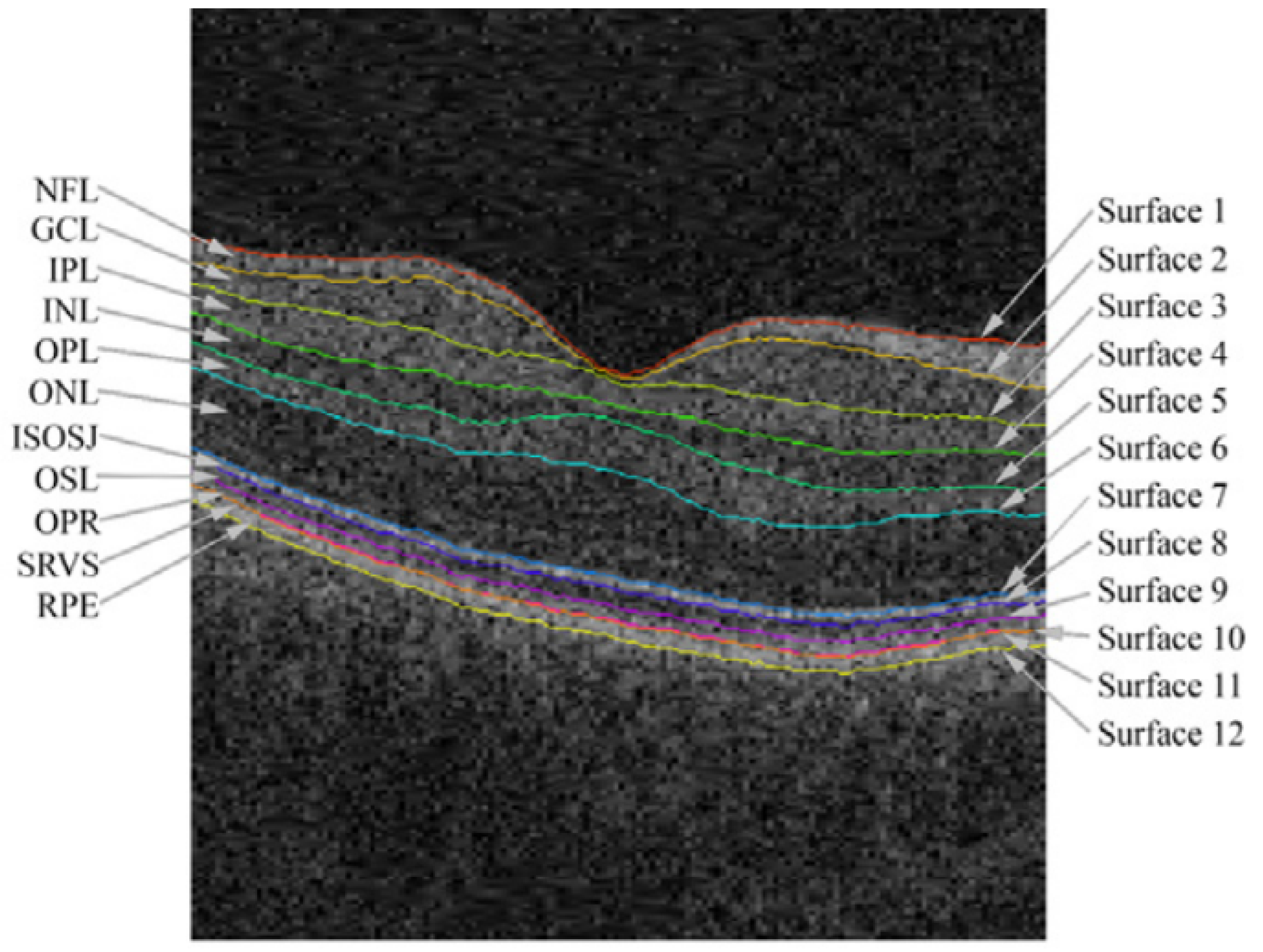
1.5. Retinal Layers
2. Background Concepts
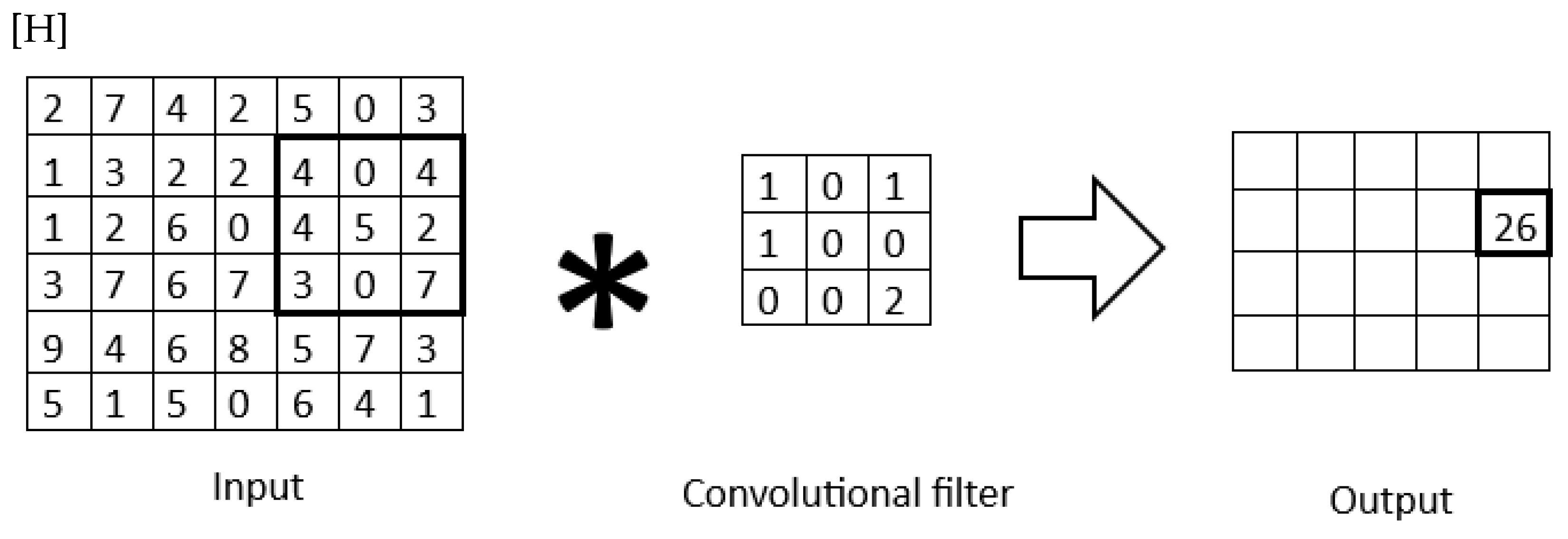
2.1. Convolutional Neural Networks
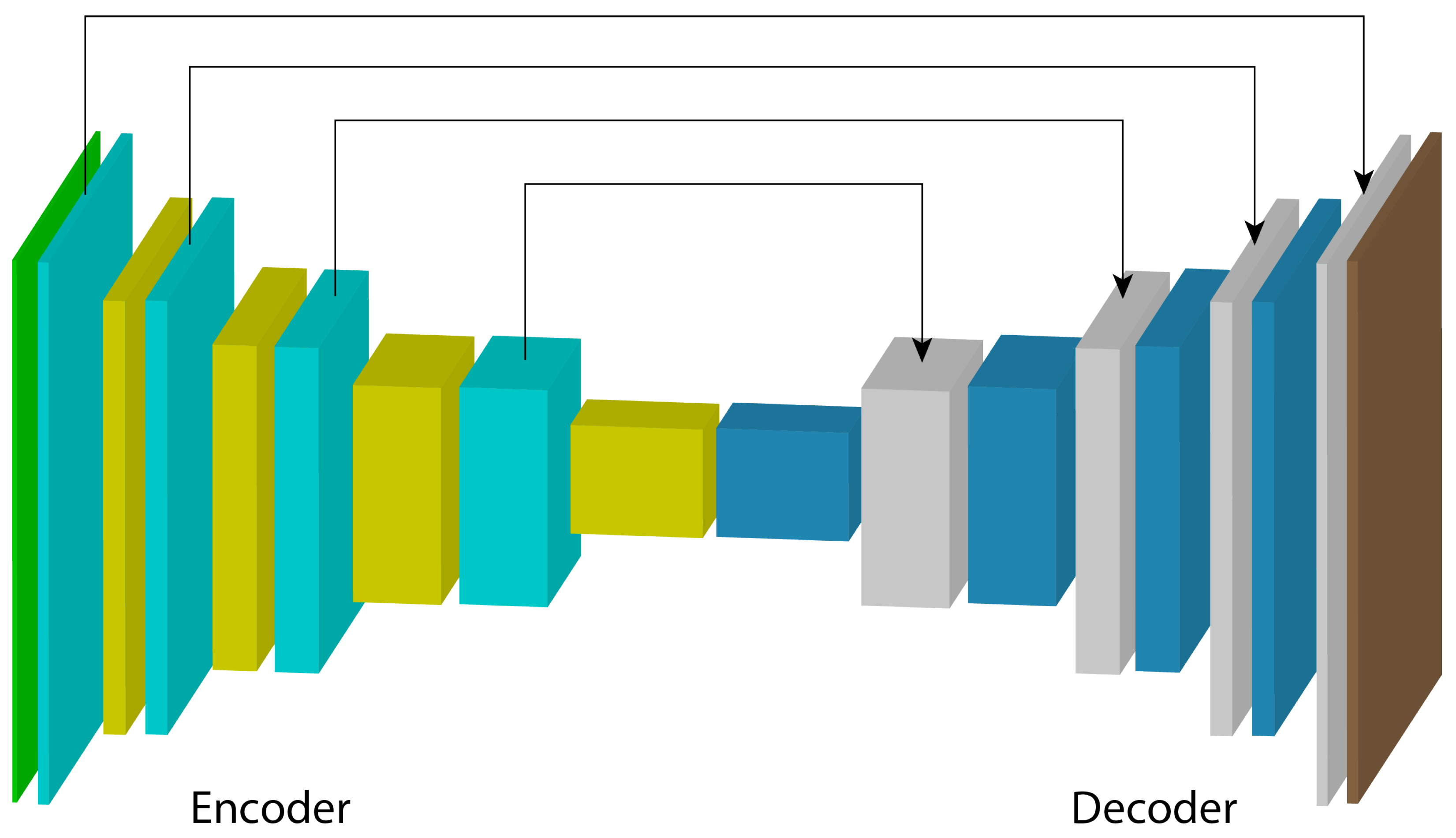
U-Net
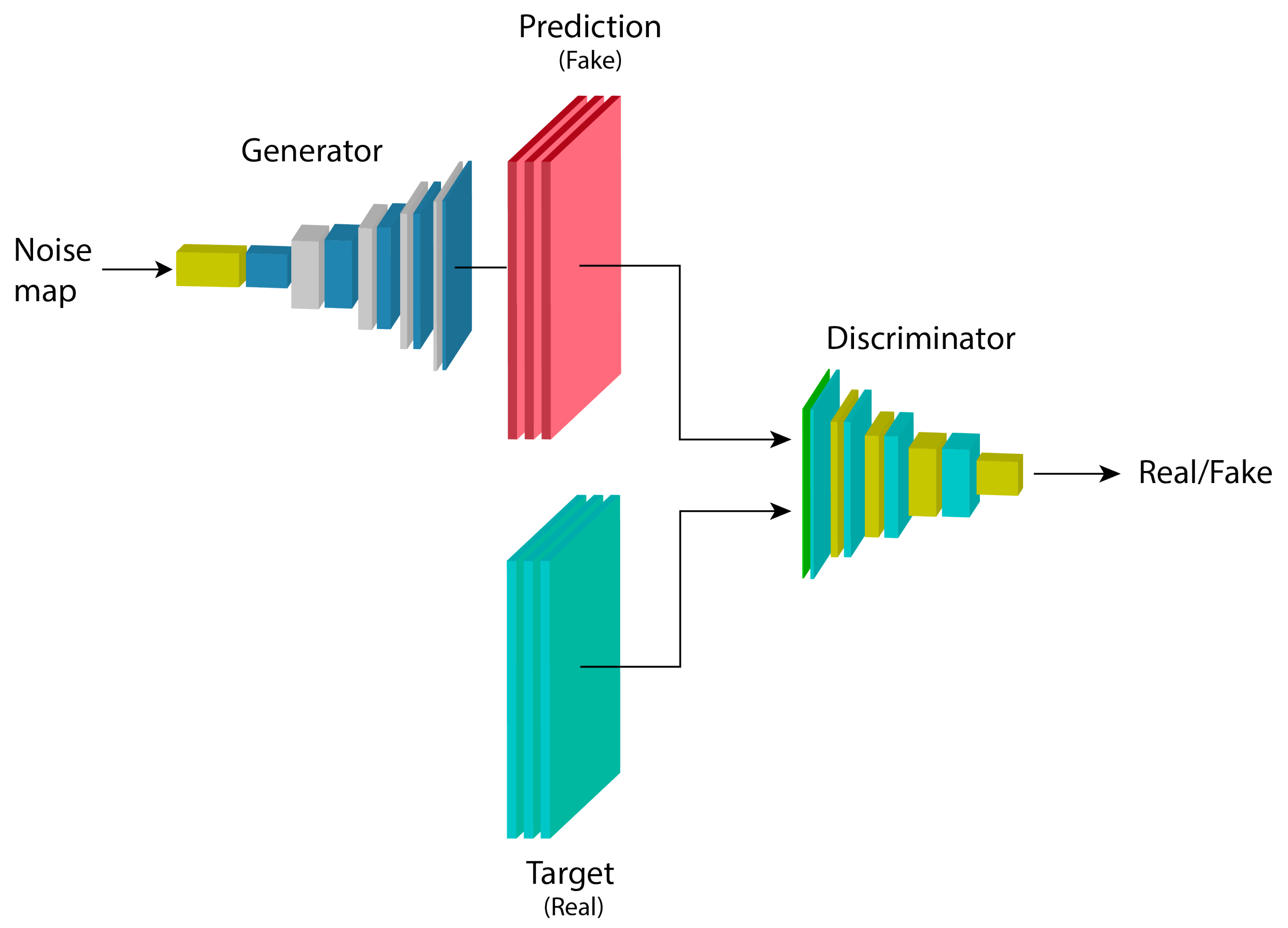
2.2. Generative Adversarial Networks
2.3. Conditional Generative Adversarial Networks
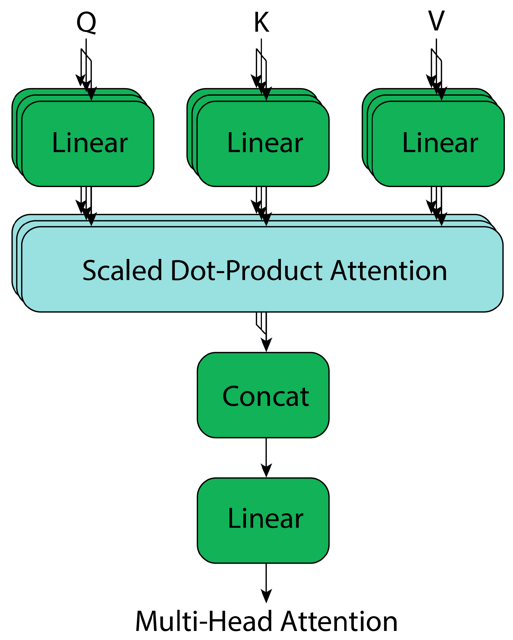
2.4. Transformers
Attention Block
3. Materials and Methods
3.1. Eligibility Criteria
- Optical Coherence Tomography OCT-based segmentation;
- Retinal layer(s);
- Segmentation/Detection;
- Deep learning/Neural network(s)/Machine learning/Artificial intelligence;
- Glaucoma/Diabetic retinopathy/Macular degeneration.
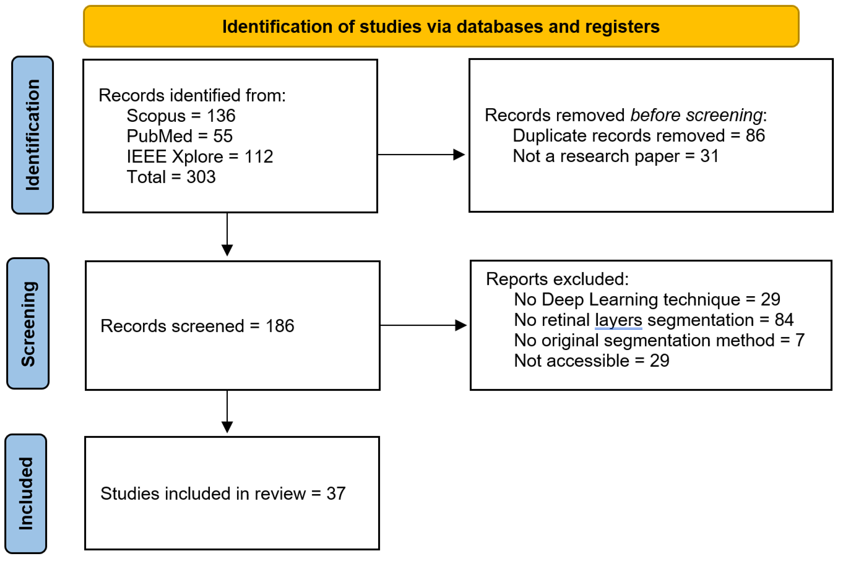
3.2. Study Selection
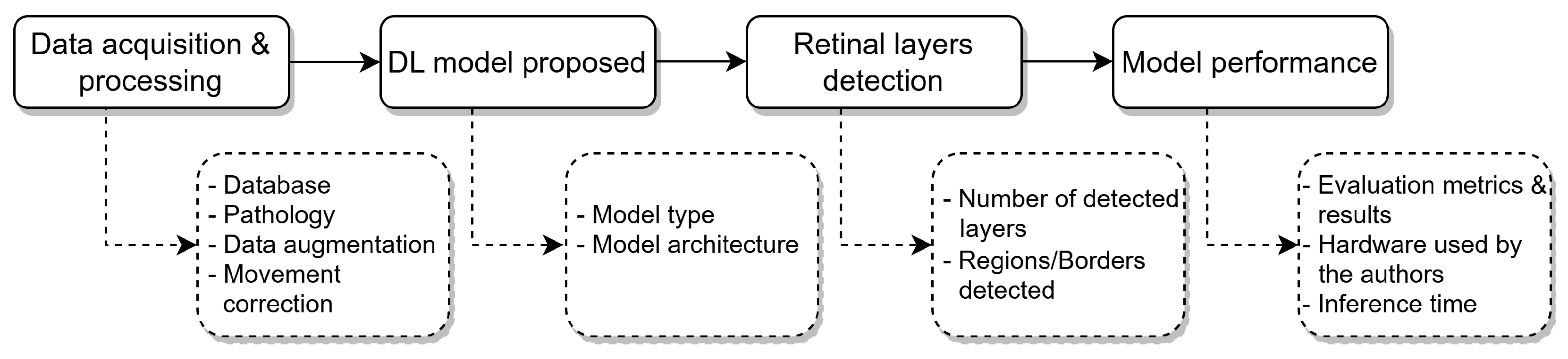
3.3. Data Extraction
3.4. Risk-of-Bias Assessment
4. Results
4.1. Data Acquisition and Processing
OCT Databases
- AFIO database [42]. The OCT and fundus images database obtained from the Armed Forces Institute of Ophthalmology (AFIO) contains ONH-centered OCT and fundus images for glaucoma detection. It includes images from healthy and glaucomatous subjects, and manual annotations for the RPE and ILM retinal layers, along with the CDR values annotated by glaucoma specialists.
- U. of Miami [43]. The OCT data from the University of Miami was obtained at the Bascom Palmer Eye Institute, which contains OCT images from subjects with diabetes. The database contains the annotations for 11 retinal boundaries (10 layers): PRS-NFL, NFL-GCL, GCL-IPL, IPL-INL, INL-OPL, OPL-HFLONL, HFLONL-ELMMYZ, ELMMYZ-ELZOS, ELZOS-IDZ, IDZ-RPE, RPE-CRC.
- Duke University-AMD [44]. The data was collected in four clinics: Devers Eye Institute, Duke Eye Center, Emory Eye Center, and National Eye Institute, containing OCT images from healthy subjects and others with intermediate and advanced AMD, aged between 50 and 85 years old. The annotations made by the authors correspond to the ILM, inner RPEDC, and outer Bruch’s membrane.
- OCT MS and Healthy Controls Data [45]. The dataset collected in the Johns Hopkins Hospital contains OCT images including healthy subjects and patients with multiple sclerosis. The dataset includes manual delineations for the following retinal layers: RNFL, GCL+IPL, INL, OPL, ONL, IS, OS, RPE.
- Duke University-DME [46]. The OCT images were acquired from patients identified in the Duke Eye Center Medical Retina with DME, for a posterior manual segmentation to segment fluid and eight retinal boundaries that result in seven regions: NFL, GCL-IPL, INL, OPL, ONL-ISM, ISE, OS-RPE.
- AROI [47]. The Annotated Retinal Optical Coherence Tomography Images (AROI) database collected at the University Hospital Center, Croatia, contains OCT images from 60-year-old subjects and older diagnosed with nAMD. The annotated retinal layers in the data include ILM, IPL-INL, RPE, and BM, along with three fluid classes.
- OCTID [48]. The Optical Coherence Tomography Image Database (OCTID) contains fovea-centered images from healthy subjects and with different diseases, such as AMD, CSR, DR, and MH, collected at Sankara Nethralaya (SN) Eye Hospital, India. The authors of the dataset include also a GUI to perform/refine the annotations for the samples. Additionally, He et al. [49] performed the layers labeling for the NFL, GCL + IPL, INL, OPL, ONL, ELM + IS, OS, and RPE retinal layers, available upon request to the authors.
- IOVS [50]. The Investigative Ophthalmology and Visual Science database includes OCT images from subjects with AMD, collected in 4 different clinics (Devers Eye Institute, Duke Eye Center, Emory Eye Center, and the National Eye Institute), and includes annotations for the ILM, RPE + drusen complex, and Bruch’s membrane structures.
4.2. Deep Learning Methods for Retinal Layers Detection
4.2.1. Convolutional Neural Networks

| Database | Layers Labeled | Number of Subjects | Demography | Subjects Conditions | Scanner | Number of Samples | Sample Resolution (pixels) | Voxel Resolution (μm/pixel) |
|---|---|---|---|---|---|---|---|---|
| AFIO [42] | ILM, RPE | 26 | Male and female. Different age groups | 32 glaucomatous, 18 healthy | TOPCON 3D OCT-1000 (Topcon Corporation, Tokio, Japan) | 50 images | 951 × 456 | - |
| U. of Miami [43] | PRS, NFL, GCL, IPL, INL, OPL, HFLONL, ELMMYZ, ELZOS, IDZ, RPE, CRC | 10 | 6 male and 4 female aged 53 ± 6 years old | All diabetic subjects | Spectralis SD-OCT (Heidelberg Engineering, Heidelberg, Germany) | 10 volumes | 768 × 61 × 496 | 11.11 × 3.87 |
| Duke University-AMD [44] | ILM, RPEDC, Outer Bruch’s membrane | 384 | Normal subjects aged 51 to 83 years old. Subjects with AMD aged 51 to 87 years old | 269 intermediate AMD, 115 healthy | SD-OCT imaging systems from Bioptigen, Inc. Research Triangle Park, NC, USA | 38,400 images | 100 × 1000 (resampled to 1001 × 1001) | 6.70 × 3.24 |
| OCT MS and Healthy Controls Data [45] | RNFL, GCL + IPL, INL, OPL, ONL, IS, OS, RPE | 35 | 6 male and 29 female aged 39.49 mean, 10.94 SD years old | 21 multiple sclerosis, 14 healthy | Spectralis OCT system (Heidelberg Engineering, Heidelberg, Germany) | 35 volumes | 49 × 496 × 1024 | 5.8 (±0.2) × 3.9 (±0.0) × 123.6 (±3.6) |
| Duke University-DME [46] | NFL, GCL-IPL, INL, OPL, ONL-ISM, ISE, OS-RPE, BM | 10 | - | All subjects with DME | Spectralis (Heidelberg Engineering, Heidelberg, Germany) | 10 volumes | 496 × 768 × 61 | 3.87 × 11.07–11.59 × 118–128 |
| AROI [47] | ILM, IPL-INL, RPE, BM | 24 | Subjects aged 60 and older | All subjects with nAMD | Zeiss Cirrus HD OCT 4000 device (Zeiss, Oberkochen, Germany) | 3072 images (1136 labelled) | 1024 × 512 | 1.96 × 11.74 × 47.24 |
| OCTID [48] | NFL, GCL + IPL, INL, OPL, ONL, ELM + IS, OS, RPE | - | - | 102 MH, 55 AMD, CSR, 107 DR, 206 healthy | Cirrus HD-OCT machine (US Ophthalmic, Miami, US) | 470 images (25 labelled) | 500 × 750 | 5 × 15 |
| IOVS [50] | ILM, RPEDC, Bruch’s membrane | 20 | - | All subjects with AMD | SD-OCT imaging systems from Bioptigen, Inc. (Research Triangle Park, NC, USA) | 25 volumes | 1000 × 512 × 100 | 3.06–3.24 × 6.50–6.60 × 65.0–69.8 |
4.2.2. U-Net-Based Architectures
4.2.3. U-Net Modifications for Retinal Layer Segmentation
- Dice Loss: Based on the Dice coefficient, this loss is used for mask segmentation, maximizing the overlap between the predicted and ground truth masks. It is particularly useful in cases of class imbalance [58,59,60,61]. The Dice loss is defined as shown in Equation (5), where represents the predicted value for pixel i, is the corresponding ground truth value, and N is the total number of pixels in the mask.
- Mean Squared Error (MSE): This loss function is used in shape regression methods to predict signed distance maps (SDMs), representing the distance to object boundaries. It is also used to directly predict the positions of retinal layer surfaces [60,62,63,64]. The MSE Loss is mathematically defined as shown in Equation (6), where and denote the ground truth and predicted values for pixel i, respectively, and N is the total number of pixels.
- Cross-Entropy Loss: This loss is used for pixel-wise classification, where each pixel is assigned to a layer, background, or fluid region. It calculates the difference between the predicted and actual probability distribution. Some studies modify or combine it with other functions [58,61,62,66]. For a binary classification problem, the cross-entropy loss is expressed as shown in Equation (7), where is the ground truth label for pixel i, is the predicted probability for the positive class, and N is the total number of pixels.
4.3. Graph-Based Methods
4.4. Generative Models
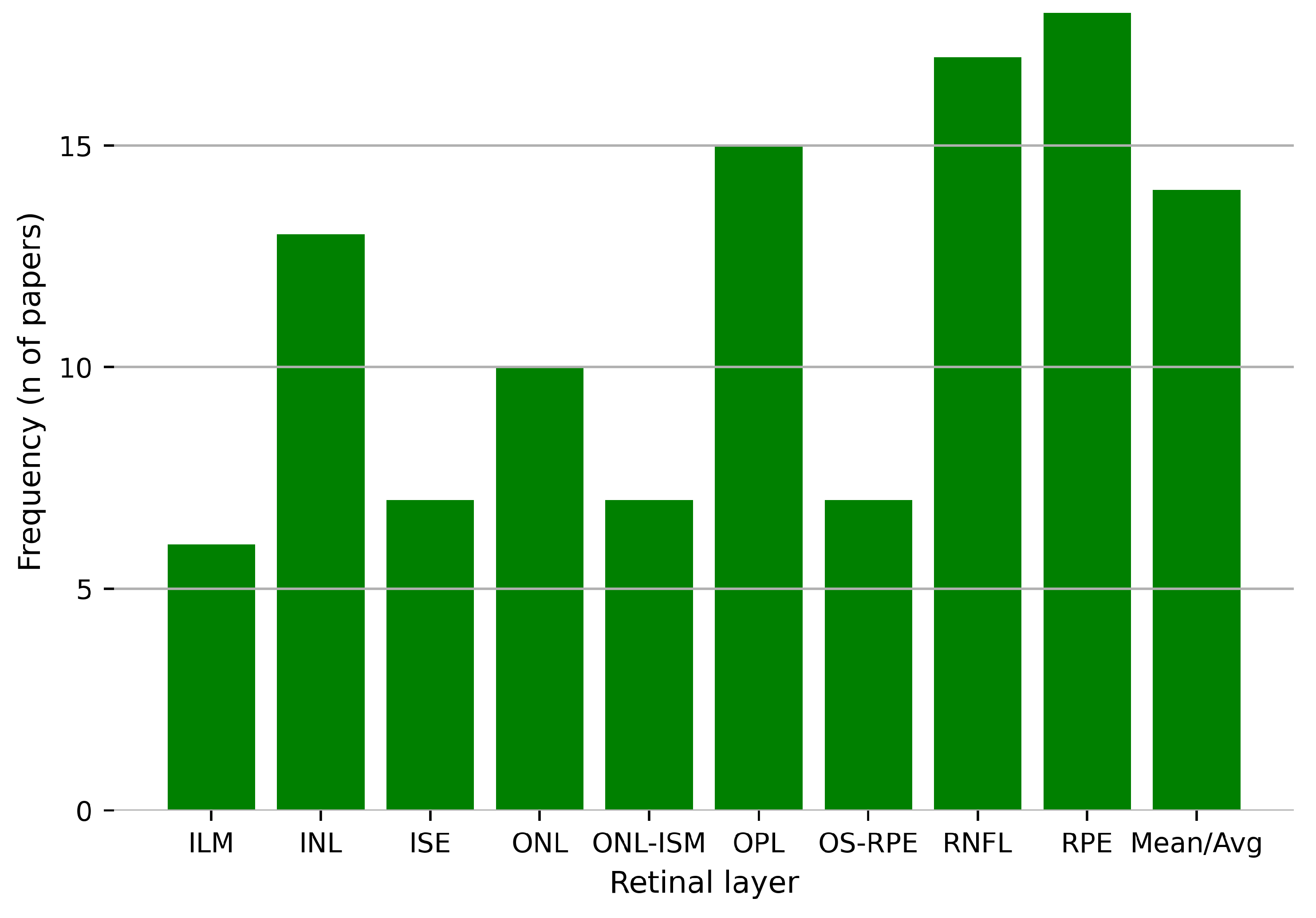
4.5. Retinal Layers Detection
4.5.1. Evaluation Metrics
4.5.2. Data Preprocessing
- Rotation: Slightly rotates images to simulate variability in acquisition angles.
- Translation: Shifts images horizontally or vertically to reduce positional bias.
- Horizontal Flip: Mirrors images horizontally to increase sample diversity.
- Vertical Crop: Extracts specific vertical sections of the image to focus on relevant regions.
- Random Crop: Selects random sections of the image to enhance spatial variability.
- Random Shearing: Applies slight angular distortions to simulate realistic deformations.
- Gaussian Noise: Adds subtle pixel-level noise to simulate sensor variability and reduce overfitting.
- Salt-and-Pepper Noise: Introduces random white and black pixel noise to improve robustness against artifacts.
- Additive Blur: Slightly blurs the image to mimic imperfections during image acquisition.
- Contrast Adjustment: Modifies image contrast to account for lighting variability during acquisition.
4.6. Model Performance
5. Discussion
5.1. Strengths and Innovations
5.2. Challenges and Limitations
5.3. Clinical Relevance and Impact
5.4. Future Research Directions
- Dataset expansion and standardization: Collaborative efforts to develop large, diverse, and publicly available datasets with standardized annotations will improve model training and evaluation. Beyond simple collection, this includes the use of generative models to create realistic synthetic OCT images. This is particularly valuable for augmenting datasets with rare pathologies or simulating variations from different scanner types, improving model robustness without compromising patient privacy. Furthermore, advanced augmentation techniques, such as elastic deformations and random nonlinear transformations, can create more challenging and realistic training scenarios.
- Improved generalization: Incorporating domain adaptation techniques and augmenting datasets with diverse pathological cases can improve the robustness of models across different populations and imaging systems. This can be achieved through unsupervised methods that learn to align feature distributions from different domains (e.g., scanners or hospitals) or by using data normalization strategies that standardize intensity profiles and reduce scanner-specific artifacts before model training.
- Hybrid architectures: Using the strengths of hybrid models that combine convolutional and attention-based mechanisms remains a promising direction. Future work could also explore vision-language models that integrate textual clinical reports with OCT images to provide contextual priors, potentially improving segmentation accuracy in ambiguous cases.
- Enhanced segmentation of challenging layers: To improve accuracy for complex layers like OPL and RNFL, research should move beyond standard loss functions. This involves exploring advanced, boundary-aware loss functions that heavily penalize errors at layer interfaces, or topology-aware losses that explicitly preserve the structural integrity and continuity of thin layers.
- Real-Time Implementation: Efforts to optimize model efficiency for deployment on edge devices or cloud-based platforms can facilitate their integration into clinical workflows, especially in under-resourced environments.
6. Conclusions
Author Contributions
Funding
Data Availability Statement
Acknowledgments
Conflicts of Interest
Abbreviations
| AACG | Acute Angle-Closure Glaucoma |
| AMD | Age-related Macular Degeneration |
| ASSD | Average Symmetric Surface Distance |
| CDR | Cup to disc ration |
| CSR | Central Serous Retinopathy |
| cGAN | Conditional Generative Adversarial Networks |
| CNN | Convolutional Neural Network |
| GAN | Generative Adversarial Network |
| DL | Deep Learning |
| DR | Diabetic Retinopathy |
| FCN | Fully Convolutional Network |
| HD | Hausdorff Distance |
| IOU | Intersection over Union |
| IOP | Intraocular pressure |
| IRF | Intraretinal fluid |
| MH | Macular Hole |
| MAD | Mean Absolute Deviation |
| MAE | Mean Absolute Error |
| MASD | Mean Absolute Surface Distance |
| mIOU | Mean Intersection over Union |
| mPA | Mean Pixel Accuracy |
| MSE | Mean Squared Error |
| MUE | Mean Unsigned Error |
| NPDR | Nonproliferative Diabetic Retinopathy |
| OCT | Optical Coherence Tomography |
| ONH | Optical nerve head |
| PED | Pigment epithelial detachment |
| PDR | Proliferative Diabetic Retinopathy |
| POAG | Primary Open-Angle Glaucoma |
| RGC | Retinal Ganglion Cells |
| RMSE | Root Mean Square Error |
| SRF | Subretinal fluid |
| UASSD | Uniform Average Symmetric Surface Distance |
| UMSP | Uniform Mean Surface Position |
| UMSPE | Uniform Mean Surface Position Error |
| USPE | Uniform Surface Position Error |
| WHO | World Health Organization |
References
- Resnikoff, S.; Pascolini, D.; Etya’ale, D.; Kocur, I.; Pararajasegaram, R.; Pokharel, G.P.; Mariotti, S.P. Global data on visual impairment in the year 2002. Bull. World Health Organ. 2004, 82, 844–851. [Google Scholar]
- Shaarawy, T.M.; Sherwood, M.B.; Hitchings, R.A.; Crowston, J.G. Glaucoma, 2nd ed.; Elsevier Health Sciences: Amsterdam, The Netherlands, 2015. [Google Scholar] [CrossRef]
- Tham, Y.C.; Li, X.; Wong, T.Y.; Quigley, H.A.; Aung, T.; Cheng, C.Y. Global Prevalence of Glaucoma and Projections of Glaucoma Burden through 2040. Ophthalmology 2014, 121, 2081–2090. [Google Scholar] [CrossRef]
- Cifuentes-Canorea, P.; Ruiz-Medrano, J.; Gutierrez-Bonet, R.; Peña-Garcia, P.; Saenz-Frances, F.; Garcia-Feijoo, J.; Martinez-de-la Casa, J.M. Analysis of inner and outer retinal layers using spectral domain optical coherence tomography automated segmentation software in ocular hypertensive and glaucoma patients. PLoS ONE 2018, 13, e0196112. [Google Scholar] [CrossRef]
- Khaw, P.; Elkington, A. Glaucoma—1: Diagnosis. BMJ 2004, 328, 97–99. [Google Scholar] [CrossRef] [PubMed]
- Weinreb, R.N.; Leung, C.K.; Crowston, J.G.; Medeiros, F.A.; Friedman, D.S.; Wiggs, J.L.; Martin, K.R. Primary open-angle glaucoma. Nat. Rev. Dis. Prim. 2016, 2, 1–19. [Google Scholar] [CrossRef] [PubMed]
- Kwon, Y.H.; Fingert, J.H.; Kuehn, M.H.; Alward, W.L. Primary open-angle glaucoma. N. Engl. J. Med. 2009, 360, 1113–1124. [Google Scholar] [CrossRef] [PubMed]
- Weinreb, R.N.; Khaw, P.T. Primary open-angle glaucoma. Lancet 2004, 363, 1711–1720. [Google Scholar] [CrossRef]
- Choong, Y.F.; Irfan, S.; Menage, M.J. Acute angle closure glaucoma: An evaluation of a protocol for acute treatment. Eye 1999, 13, 613–616. [Google Scholar] [CrossRef]
- Lim, L.S.; Mitchell, P.; Seddon, J.M.; Holz, F.G.; Wong, T.Y. Age-related macular degeneration. Lancet 2012, 379, 1728–1738. [Google Scholar] [CrossRef]
- Fong, D.S.; Aiello, L.; Gardner, T.W.; King, G.L.; Blankenship, G.; Cavallerano, J.D.; Ferris, F.L.; Klein, R.; Association, A.D. Retinopathy in Diabetes. Diabetes Care 2004, 27, s84–s87. [Google Scholar] [CrossRef]
- Drexler, W.; Fujimoto, J.G. (Eds.) Optical Coherence Tomography: Technology and Applications, 2nd ed.; Springer International Publishing: Cham, Switzerland, 2015. [Google Scholar] [CrossRef]
- Huang, D.; Swanson, E.A.; Lin, C.P.; Schuman, J.S.; Stinson, W.G.; Chang, W.; Hee, M.R.; Flotte, T.; Gregory, K.; Puliafito, C.A.; et al. Optical Coherence Tomography. Science 1991, 254, 1178–1181. [Google Scholar] [CrossRef]
- Mashige, K.P.; Oduntan, O.A. A review of the human retina with emphasis on nerve fibre layer and macula thicknesses. Afr. Vis. Eye Health 2016, 75, 1–8. [Google Scholar] [CrossRef]
- Hildebrand, G.D.; Fielder, A.R. Anatomy and physiology of the retina. In Pediatric Retina; Springer: Berlin/Heidelberg, Germany, 2010; pp. 39–65. [Google Scholar]
- Nguyen, K.; Patel, B.; Tadi, P. Anatomy, Head and Neck: Eye Retina. In StatPearls [Internet]; StatPearls Publishing: Treasure Island, FL, USA, 2025. [Google Scholar]
- Masri, R.A.; Weltzien, F.; Purushothuman, S.; Lee, S.C.; Martin, P.R.; Grünert, U. Composition of the inner nuclear layer in human retina. Investig. Ophthalmol. Vis. Sci. 2021, 62, 22. [Google Scholar] [CrossRef]
- Kim, S.Y.; Park, C.H.; Moon, B.H.; Seabold, G.K. Murine Retina Outer Plexiform Layer Development and Transcriptome Analysis of Pre-Synapses in Photoreceptors. Life 2024, 14, 1103. [Google Scholar] [CrossRef]
- Mahabadi, N.; Al Khalili, Y. Neuroanatomy, Retina. In StatPearls [Internet]; StatPearls Publishing: Treasure Island, FL, USA, 2025. [Google Scholar]
- Lujan, B.J.; Roorda, A.; Croskrey, J.A.; Dubis, A.M.; Cooper, R.F.; Bayabo, J.K.; Duncan, J.L.; Antony, B.J.; Carroll, J. Directional optical coherence tomography provides accurate outer nuclear layer and Henle fiber layer measurements. Retina 2015, 35, 1511–1520. [Google Scholar] [CrossRef]
- Landa, G.; Gentile, R.; Garcia, P.; Muldoon, T.; Rosen, R. External limiting membrane and visual outcome in macular hole repair: Spectral domain OCT analysis. Eye 2012, 26, 61–69. [Google Scholar] [CrossRef]
- Saxena, S.; Akduman, L.; Meyer, C.H. External limiting membrane: Retinal structural barrier in diabetic macular edema. Int. J. Retin. Vitr. 2021, 7, 1–3. [Google Scholar] [CrossRef]
- Chen, X.; Zhang, L.; Sohn, E.H.; Lee, K.; Niemeijer, M.; Chen, J.; Sonka, M.; Abramoff, M.D. Quantification of external limiting membrane disruption caused by diabetic macular edema from SD-OCT. Investig. Ophthalmol. Vis. Sci. 2012, 53, 8042–8048. [Google Scholar] [CrossRef] [PubMed]
- Narayan, D.S.; Chidlow, G.; Wood, J.P.; Casson, R.J. Glucose metabolism in mammalian photoreceptor inner and outer segments. Clin. Exp. Ophthalmol. 2017, 45, 730–741. [Google Scholar] [CrossRef] [PubMed]
- Yang, S.; Zhou, J.; Li, D. Functions and diseases of the retinal pigment epithelium. Front. Pharmacol. 2021, 12, 727870. [Google Scholar] [CrossRef] [PubMed]
- Sonka, M.; Abràmoff, M.D. Quantitative analysis of retinal OCT. Med. Image Anal. 2016, 33, 165–169. [Google Scholar] [CrossRef]
- Jeoung, J.W.; Park, K.H. Comparison of Cirrus OCT and Stratus OCT on the Ability to Detect Localized Retinal Nerve Fiber Layer Defects in Preperimetric Glaucoma. Investig. Opthalmology Vis. Sci. 2010, 51, 938. [Google Scholar] [CrossRef]
- Yamada, H.; Hangai, M.; Nakano, N.; Takayama, K.; Kimura, Y.; Miyake, M.; Akagi, T.; Ikeda, H.O.; Noma, H.; Yoshimura, N. Asymmetry Analysis of Macular Inner Retinal Layers for Glaucoma Diagnosis. Am. J. Ophthalmol. 2014, 158, 1318–1329.e3. [Google Scholar] [CrossRef]
- LeCun, Y.; Bengio, Y.; Hinton, G. Deep learning. Nature 2015, 521, 436–444. [Google Scholar] [CrossRef] [PubMed]
- Aggarwal, C.C. Neural Networks and Deep Learning: A Textbook; Springer International Publishing: Cham, Switzerland, 2018. [Google Scholar] [CrossRef]
- Bengio, Y.; Goodfellow, I.; Courville, A. Deep Learning; MIT Press: Cambridge, MA, USA, 2017; Volume 1. [Google Scholar]
- Charniak, E. Introduction to Deep Learning; Cambridge University Press: Cambridge, UK, 2019; Volume 53, pp. 1689–1699. [Google Scholar] [CrossRef]
- Krizhevsky, A.; Sutskever, I.; Hinton, G.E. ImageNet classification with deep convolutional neural networks. Commun. ACM 2017, 60, 84–90. [Google Scholar] [CrossRef]
- Ronneberger, O.; Fischer, P.; Brox, T. U-net: Convolutional networks for biomedical image segmentation. In Proceedings of the Medical Image Computing and Computer-Assisted Intervention–MICCAI 2015: 18th International Conference, Munich, Germany, 5–9 October 2015; proceedings, part III 18. Springer: Berlin/Heidelberg, Germany, 2015; pp. 234–241. [Google Scholar]
- Goodfellow, I.; Pouget-Abadie, J.; Mirza, M.; Xu, B.; Warde-Farley, D.; Ozair, S.; Courville, A.; Bengio, Y. Generative Adversarial Nets. In Proceedings of the Advances in Neural Information Processing Systems; Ghahramani, Z., Welling, M., Cortes, C., Lawrence, N., Weinberger, K., Eds.; Curran Associates, Inc.: Red Hook, NY, USA, 2014; Volume 27. [Google Scholar]
- Isola, P.; Zhu, J.Y.; Zhou, T.; Efros, A.A. Image-to-Image Translation with Conditional Adversarial Networks. In Proceedings of the IEEE Conference on Computer Vision and Pattern Recognition (CVPR), Honolulu, HI, USA, 21–26 July 2017. [Google Scholar]
- Vaswani, A. Attention is all you need. Adv. Neural Inf. Process. Syst. 2017, 30. [Google Scholar]
- Dosovitskiy, A.; Beyer, L.; Kolesnikov, A.; Weissenborn, D.; Zhai, X.; Unterthiner, T.; Dehghani, M.; Minderer, M.; Heigold, G.; Gelly, S.; et al. An Image is Worth 16 × 16 Words: Transformers for Image Recognition at Scale. arXiv 2021, arXiv:2010.11929. [Google Scholar]
- Liu, Z.; Lin, Y.; Cao, Y.; Hu, H.; Wei, Y.; Zhang, Z.; Lin, S.; Guo, B. Swin Transformer: Hierarchical Vision Transformer using Shifted Windows. In Proceedings of the IEEE/CVF International Conference on Computer Vision (ICCV), Montreal, QC, Canada, 10–17 October 2021; pp. 9992–10002. [Google Scholar]
- Dong, X.; Bao, J.; Chen, D.; Zhang, W.; Yu, N.; Yuan, L.; Chen, D.; Guo, B. CSWin Transformer: A General Vision Transformer Backbone with Cross-Shaped Windows. In Proceedings of the IEEE/CVF Conference on Computer Vision and Pattern Recognition (CVPR), New Orleans, LA, USA, 18–24 June 2022; pp. 12114–12124. [Google Scholar]
- Page, M.J.; McKenzie, J.E.; Bossuyt, P.M.; Boutron, I.; Hoffmann, T.C.; Mulrow, C.D.; Shamseer, L.; Tetzlaff, J.M.; Akl, E.A.; Brennan, S.E.; et al. The PRISMA 2020 statement: An updated guideline for reporting systematic reviews. BMJ 2021, 372, n71. [Google Scholar] [CrossRef]
- Raja, H.; Akram, M.U.; Khawaja, S.G.; Arslan, M.; Ramzan, A.; Nazir, N. Data on OCT and fundus images for the detection of glaucoma. Data Brief 2020, 29, 105342. [Google Scholar] [CrossRef]
- Tian, J.; Varga, B.; Tatrai, E.; Fanni, P.; Somfai, G.M.; Smiddy, W.E.; Debuc, D.C. Performance evaluation of automated segmentation software on optical coherence tomography volume data. J. Biophotonics 2016, 9, 478–489. [Google Scholar] [CrossRef]
- Farsiu, S.; Chiu, S.J.; O’Connell, R.V.; Folgar, F.A.; Yuan, E.; Izatt, J.A.; Toth, C.A. Quantitative Classification of Eyes with and without Intermediate Age-related Macular Degeneration Using Optical Coherence Tomography. Ophthalmology 2014, 121, 162–172. [Google Scholar] [CrossRef]
- He, Y.; Carass, A.; Solomon, S.D.; Saidha, S.; Calabresi, P.A.; Prince, J.L. Retinal layer parcellation of optical coherence tomography images: Data resource for multiple sclerosis and healthy controls. Data Brief 2019, 22, 601–604. [Google Scholar] [CrossRef] [PubMed]
- Chiu, S.J.; Allingham, M.J.; Mettu, P.S.; Cousins, S.W.; Izatt, J.A.; Farsiu, S. Kernel regression based segmentation of optical coherence tomography images with diabetic macular edema. Biomed. Opt. Express 2015, 6, 1172. [Google Scholar] [CrossRef] [PubMed]
- Melinščak, M.; Radmilović, M.; Vatavuk, Z.; Lončarić, S. Annotated retinal optical coherence tomography images (AROI) database for joint retinal layer and fluid segmentation. Automatika 2021, 62, 375–385. [Google Scholar] [CrossRef]
- Gholami, P.; Roy, P.; Parthasarathy, M.K.; Lakshminarayanan, V. OCTID: Optical coherence tomography image database. Comput. Electr. Eng. 2020, 81, 106532. [Google Scholar] [CrossRef]
- He, X.; Wang, Y.; Poiesi, F.; Song, W.; Xu, Q.; Feng, Z.; Wan, Y. Exploiting multi-granularity visual features for retinal layer segmentation in human eyes. Front. Bioeng. Biotechnol. 2023, 11, 1191803. [Google Scholar] [CrossRef]
- Chiu, S.J.; Izatt, J.A.; O’Connell, R.V.; Winter, K.P.; Toth, C.A.; Farsiu, S. Validated Automatic Segmentation of AMD Pathology Including Drusen and Geographic Atrophy in SD-OCT Images. Investig. Opthalmology Vis. Sci. 2012, 53, 53. [Google Scholar] [CrossRef]
- Shah, A.; Zhou, L.; Abrámoff, M.D.; Wu, X. Multiple surface segmentation using convolution neural nets: Application to retinal layer segmentation in OCT images. Biomed. Opt. Express 2018, 9, 4509–4526. [Google Scholar] [CrossRef]
- Raja, H.; Akram, M.U.; Shaukat, A.; Khan, S.A.; Alghamdi, N.; Khawaja, S.G.; Nazir, N. Extraction of Retinal Layers Through Convolution Neural Network (CNN) in an OCT Image for Glaucoma Diagnosis. J. Digit. Imaging 2020, 33, 1428–1442. [Google Scholar] [CrossRef]
- Cansiz, S.; Kesim, C.; Bektas, S.N.; Kulali, Z.; Hasanreisoglu, M.; Gunduz-Demir, C. FourierNet: Shape-Preserving Network for Henle’s Fiber Layer Segmentation in Optical Coherence Tomography Images. IEEE J. Biomed. Health Inform. 2023, 27, 1036–1047. [Google Scholar] [CrossRef]
- Hu, K.; Shen, B.; Zhang, Y.; Cao, C.; Xiao, F.; Gao, X. Automatic segmentation of retinal layer boundaries in OCT images using multiscale convolutional neural network and graph search. Neurocomputing 2019, 365, 302–313. [Google Scholar] [CrossRef]
- Cazañas-Gordón, A.; Cruz, L.A.d.S. Multiscale Attention Gated Network (MAGNet) for Retinal Layer and Macular Cystoid Edema Segmentation. IEEE Access 2022, 10, 3198657. [Google Scholar] [CrossRef]
- Wang, J.; Wang, Z.; Li, F.; Qu, G.; Qiao, Y.; Lv, H.; Zhang, X. Joint retina segmentation and classification for early glaucoma diagnosis. Biomed. Opt. Express 2019, 10, 2639–2656. [Google Scholar] [CrossRef] [PubMed]
- He, Y.; Carass, A.; Liu, Y.; Jedynak, B.M.; Solomon, S.D.; Saidha, S.; Calabresi, P.A.; Prince, J.L. Structured layer surface segmentation for retina OCT using fully convolutional regression networks. Med. Image Anal. 2021, 68, 101856. [Google Scholar] [CrossRef] [PubMed]
- Fazekas, B.; Aresta, G.; Lachinov, D.; Riedl, S.; Mai, J.; Schmidt-Erfurth, U.; Bogunović, H. SD-LayerNet: Semi-supervised Retinal Layer Segmentation in OCT Using Disentangled Representation with Anatomical Priors. In Medical Image Computing and Computer Assisted Intervention—MICCAI 2022; Springer: Cham, Switzerland, 2022; Volume 13438. [Google Scholar] [CrossRef]
- Cao, J.; Liu, X.; Zhang, Y.; Wang, M. A Multi-task Framework for Topology-guaranteed Retinal Layer Segmentation in OCT Images. In Proceedings of the 2020 IEEE International Conference on Systems, Man, and Cybernetics (SMC), Toronto, ON, Canada, 11–14 October 2020. [Google Scholar] [CrossRef]
- Vázquez, E.R.; Rodríguez, M.N.B.; López-Varela, E.; Penedo, M.G. Deep Learning for Segmentation of Optic Disc and Retinal Layers in Peripapillary Optical Coherence Tomography Images. In Proceedings of the Fifteenth International Conference on Machine Vision (ICMV 2022), Rome, Italy, 18–20 November 2023; Volume 12701. [Google Scholar] [CrossRef]
- Matovinovic, I.Z.; Loncaric, S.; Lo, J.; Heisler, M.; Sarunic, M. Transfer learning with U-net type model for automatic segmentation of three retinal layers in optical coherence tomography images. In Proceedings of the 2019 11th International Symposium on Image and Signal Processing and Analysis, Dubrovnik, Croatia, 23–25 September 2019; Volume 2019. [Google Scholar] [CrossRef]
- Kepp, T.; Ehrhardt, J.; Heinrich, M.P.; Hüttmann, G.; Handels, H. Topology-Preserving Shape-Based Regression Of Retinal Layers In Oct Image Data Using Convolutional Neural Networks. In Proceedings of the 2019 IEEE 16th International Symposium on Biomedical Imaging (ISBI 2019), Venice, Italy, 8–11 April 2019. [Google Scholar] [CrossRef]
- Chen, Z.; Zhang, H.; Linton, E.F.; Johnson, B.A.; Choi, Y.J.; Kupersmith, M.J.; Sonka, M.; Garvin, M.K.; Kardon, R.H.; Wang, J.K. Hybrid deep learning and optimal graph search method for optical coherence tomography layer segmentation in diseases affecting the optic nerve. Biomed. Opt. Express 2024, 15, 3681–3698. [Google Scholar] [CrossRef]
- Ndipenoch, N.; Miron, A.; Wang, Z.; Li, Y. Simultaneous Segmentation of Layers and Fluids in Retinal OCT Images. In Proceedings of the 2022 15th International Congress on Image and Signal Processing, BioMedical Engineering and Informatics (CISP-BMEI), Beijing, China, 5–7 November 2022. [Google Scholar] [CrossRef]
- Moradi, M.; Chen, Y.; Du, X.; Seddon, J.M. Deep ensemble learning for automated non-advanced AMD classification using optimized retinal layer segmentation and SD-OCT scans. Comput. Biol. Med. 2023, 154, 106512. [Google Scholar] [CrossRef]
- Zhilin, Z.; Yan, W.; Zeyu, P.; Yunqing, Z.; Rugang, Y.; Guogang, C. Dual Attention Network for Retinal Layer and Fluid Segmentation in OCT. In Proceedings of the 2023 8th International Conference on Intelligent Informatics and Biomedical Sciences (ICIIBMS), Okinawa, Japan, 23–25 November 2023; Volume 8. [Google Scholar] [CrossRef]
- Mukherjee, S.; De Silva, T.; Grisso, P.; Wiley, H.; Tiarnan, D.K.; Thavikulwat, A.T.; Chew, E.; Cukras, C. Retinal layer segmentation in optical coherence tomography (OCT) using a 3D deep-convolutional regression network for patients with age-related macular degeneration. Biomed. Opt. Express 2022, 13, 3195–3210. [Google Scholar] [CrossRef]
- Xie, H.; Xu, W.; Wang, Y.X.; Wu, X. Deep learning network with differentiable dynamic programming for retina OCT surface segmentation. Biomed. Opt. Express 2023, 14, 3190–3202. [Google Scholar] [CrossRef]
- Shen, Y.; Li, J.; Zhu, W.; Yu, K.; Wang, M.; Peng, Y.; Zhou, Y.; Guan, L.; Chen, X. Graph Attention U-Net for Retinal Layer Surface Detection and Choroid Neovascularization Segmentation in OCT Images. IEEE Trans. Med. Imaging 2023, 42, 3140–3154. [Google Scholar] [CrossRef]
- Hu, K.; Liu, D.; Chen, Z.; Li, X.; Zhang, Y.; Gao, X. Embedded Residual Recurrent Network and Graph Search for the Segmentation of Retinal Layer Boundaries in Optical Coherence Tomography. IEEE Trans. Instrum. Meas. 2021, 70, 1–17. [Google Scholar] [CrossRef]
- Kugelman, J.; Alonso-Caneiro, D.; Read, S.A.; Vincent, S.J.; Collins, M.J. Automatic segmentation of OCT retinal boundaries using recurrent neural networks and graph search. Biomed. Opt. Express 2018, 9, 5759–5777. [Google Scholar] [CrossRef]
- Li, J.; Jin, P.; Zhu, J.; Zou, H.; Xu, X.; Tang, M.; Zhou, M.; Gan, Y.; He, J.; Ling, Y.; et al. Multi-scale GCN-assisted two-stage network for joint segmentation of retinal layers and discs in peripapillary OCT images. Biomed. Opt. Express 2021, 12, 2204–2220. [Google Scholar] [CrossRef] [PubMed]
- Mishra, Z.; Ganegoda, A.; Selicha, J.; Wang, Z.; Sadda, S.R.; Hu, Z. Automated Retinal Layer Segmentation Using Graph-based Algorithm Incorporating Deep-learning-derived Information. Sci. Rep. 2020, 10, 9541. [Google Scholar] [CrossRef] [PubMed]
- Li, J.; Ling, Y.; He, J.; Jin, P.; Zhu, J.; Zou, H.; Xu, X.; Shao, S.; Gan, Y.; Su, Y. A GCN-assisted deep learning method for peripapillary retinal layer segmentation in OCT images. In Proceedings of the Optical Coherence Tomography and Coherence Domain Optical Methods in Biomedicine XXV, Online, 6–11 March 2021; Volume 11630. [Google Scholar] [CrossRef]
- Fang, L.; Cunefare, D.; Wang, C.; Guymer, R.H.; Li, S.; Farsiu, S. Automatic segmentation of nine retinal layer boundaries in OCT images of non-exudative AMD patients using deep learning and graph search. Biomed. Opt. Express 2017, 8, 2732–2744. [Google Scholar] [CrossRef] [PubMed]
- Wang, Y.; Galang, C.; Freeman, W.R.; Warter, A.; Heinke, A.; Bartsch, D.U.G.; Nguyen, T.Q.; An, C. Retinal OCT Layer Segmentation via Joint Motion Correction and Graph-Assisted 3D Neural Network. IEEE Access 2023, 11, 103319–103332. [Google Scholar] [CrossRef]
- Heisler, M.; Bhalla, M.; Lo, J.; Mammo, Z.; Lee, S.; Ju, M.J.; Beg, M.F.; Sarunic, M.V. Semi-supervised deep learning based 3D analysis of the peripapillary region. Biomed. Opt. Express 2020, 11, 3843–3856. [Google Scholar] [CrossRef]
- Xue, S.; Wang, H.; Guo, X.; Sun, M.; Song, K.; Shao, Y.; Zhang, H.; Zhang, T. CTS-Net: A Segmentation Network for Glaucoma Optical Coherence Tomography Retinal Layer Images. Bioengineering 2023, 10, 230. [Google Scholar] [CrossRef]
- Tonade, D.; Kern, T.S. Photoreceptor cells and RPE contribute to the development of diabetic retinopathy. Prog. Retin. Eye Res. 2021, 83, 100919. [Google Scholar] [CrossRef]
- Wheat, J.L.; Rangaswamy, N.V.; Harwerth, R.S. Correlating RNFL thickness by OCT with perimetric sensitivity in glaucoma patients. J. Glaucoma 2012, 21, 95–101. [Google Scholar] [CrossRef]
- Morelle, O.; Wintergerst, M.W.; Finger, R.P.; Schultz, T. Accurate drusen segmentation in optical coherence tomography via order-constrained regression of retinal layer heights. Sci. Rep. 2023, 13, 8162. [Google Scholar] [CrossRef]
- Baidu AI Studio Competition: Retinal OCT Layer Segmentation. 2022. Available online: https://aistudio.baidu.com/aistudio/competition/detail/783/0/introduction (accessed on 18 December 2024).
- He, Y.; Carass, A.; Liu, Y.; Calabresi, P.A.; Saidha, S.; Prince, J.L. Longitudinal deep network for consistent OCT layer segmentation. Biomed. Opt. Express 2023, 14, 1874–1893. [Google Scholar] [CrossRef]
- Sousa, J.A.; Paiva, A.; Silva, A.; Almeida, J.D.; Braz, J.G.; Diniz, J.O.; Figueredo, W.K.; Gattass, M. Automatic segmentation of retinal layers in OCT images with intermediate age-related macular degeneration using U-Net and DexiNed. PLoS ONE 2021, 16, e0251591. [Google Scholar] [CrossRef]
- Gende, M.; de Moura, J.; Fernández-Vigo, J.I.; Martínez-de-la-Casa, J.M.; García-Feijóo, J.; Novo, J.; Ortega, M. Robust multi-view approaches for retinal layer segmentation in glaucoma patients via transfer learning. Quant. Imaging Med. Surg. 2023, 13, 2846. [Google Scholar] [CrossRef]
- Dodo, B.I.; Li, Y.; Eltayef, K.; Liu, X. Automatic annotation of retinal layers in optical coherence tomography images. J. Med. Syst. 2019, 43, 336. [Google Scholar] [CrossRef]
- Konno, T.; Ninomiya, T.; Miura, K.; Ito, K.; Himori, N.; Sharma, P.; Nakazawa, T.; Aoki, T. Retinal Layer Segmentation from Oct Images Using 2D-3D Hybrid Network with Multi-Scale Loss and Refinement Module. In Proceedings of the 2023 IEEE 20th International Symposium on Biomedical Imaging (ISBI), Cartagena, Colombia, 18–21 April 2023. [Google Scholar] [CrossRef]
- Hassan, T.; Usman, A.; Akram, M.U.; Masood, M.F.; Yasin, U. Deep Learning Based Automated Extraction of Intra-Retinal Layers for Analyzing Retinal Abnormalities. In Proceedings of the 2018 IEEE 20th International Conference on e-Health Networking, Applications and Services (Healthcom), Ostrava, Czech Republic, 17–20 September 2018. [Google Scholar] [CrossRef]
- Liu, X.; Cao, J.; Wang, S.; Zhang, Y.; Wang, M. Confidence-Guided Topology-Preserving Layer Segmentation for Optical Coherence Tomography Images with Focus-Column Module. IEEE Trans. Instrum. Meas. 2020, 70, 5005612. [Google Scholar] [CrossRef]
- Wei, H.; Peng, P. The Segmentation of Retinal Layer and Fluid in SD-OCT Images Using Mutex Dice Loss Based Fully Convolutional Networks. IEEE Access 2020, 8, 60929–60939. [Google Scholar] [CrossRef]


| Reference | Dataset Used by the Authors | N of Retinal Layers/Boundaries Detected | Retinal Layers Detected | Metrics Reported | Pathology |
|---|---|---|---|---|---|
| Shah [51] | Duke University-AMD [44] | 3 | ILM, IRPE, OBM | UMSP, UASSD | Healthy, AMD |
| Cazañas-Gordón [55] | Dataset 1: Duke University-DME [46]. Dataset 2: OCT MS and Healthy Controls Data [45] | Dataset 1: 7. Dataset 2: 8 | Dataset 1: ILM, NFL-IPL, INL, OPL, ONL-ISM, ISE, OS-RPE. Dataset 2: ILM, NFL-IPL, INL, OPL, ONL, IS, OS, RPE | Dice Score | Healthy, DME, MS |
| Xie [68] | Dataset 1: Duke University-AMD [44]. Dataset 2: OCT MS and Healthy Controls Data [45] | 3, 9 | Dataset 1: ILM, InnerRPEDC, OBM. Dataset 2: ILM, RNFL-GCL, IPL-INL, INL-OPL, OPL-ONL, ELM, IS-OS, OS-RPE, BM | MASD, HD | Healthy, AMD, MS |
| Fazekas [58] | Private | 6 | ILM, RNFL, BMEIS, RPE, RPE-BM, BM | RMSE | AMD |
| Raja [52] | AFIO (authors labeled the data) | 2 | ILM, RPE | Absolute mean error | Healthy, glaucoma |
| Hu [54] | U. of Miami [43] | 5 | RNFL, RNFL-GCL, IPL-INL, OPL-HFONL, BM (Bruch’s complex- Choriocapillaris) | MAE, MSE | DR |
| Morelle [81] | Dataset 1: Private. Dataset 2: Duke University-AMD [44] | 3 | ILM, IBRPE, BM | MAE | Healthy, AMD |
| Xue [78] | GOALS [82] | 5 | ILM, RNFL-GCIPL, GCIPL-INL, BM, CS | MAD, RMSE, Dice Score | Glaucoma |
| He [83] | Private | 9 | ILM, RNFL-GCL, IPL-INL, INP-OPL, OPL-ONL, ELM, IS-OS, OS-RPE, BM | MAD | MS |
| Shen [69] | Dataset 1: Private. Dataset 2: OCT MS and Healthy Controls Data [45] | 9 | RNFL, GCL, IPL, INL, OPL, ONL, ELM, OPSL, RPE | USPE, UMSPE | Healthy, AMD, MS |
| Heisler [77] | Private | 4 | ILM, ILM-RNFL, RNFL,BM, BM-CS, CS | Dice Score | Healthy, glaucoma |
| Moradi [65] | Dataset 1: Private. Dataset 2: Duke University-AMD [44] | 10 | ILM, RNFL, GCL, IPL, INL, OPL + HFL,EZ, IS-OS, OPR, RPE (inner & outer) | IOU, Dice Score, Precision, Sensitivity | Healthy, AMD |
| Cansiz [53] | Private | 1 | HFL | Precision, Recall, F-Score | Healthy |
| Li [74] | Private | 9 | RNFL, GCL, IPL, INL, OPL, ONL, IS-OS, RPE, Choroid | Dice Score, Accuracy | - |
| Li [72] | Dataset 1: Private. Dataset 2: Duke University-DME [46] | 9 | RNFL, GCL, IPL, INL, OPL, ONL, IS-OS, RPE, Choroid | Dice Score, Accuracy | DME |
| Mukherjee [67] | Private | 3 | ILM, RPE, BM | RMSE, MAE, HD | AMD |
| He [57] | Dataset 1: OCT MS and Healthy Controls Data [45]. Dataset 2: Duke University-DME [46] | Dataset 1: 9. Dataset 2: 8 | Dataset 1: ILM, RNFL-GCL, IPL-INL, INL-OPL, OPL-ONL, ELM, IS-OS, OS-RPE, BM. Dataset 2: ILM, RNFL-GCL, IPL-INL, INL-OPL, OPL-ONL, IS-OS, OS-RPE, BM | MAD, RMSE | Healthy, MS, DME |
| Sousa [84] | Duke University-AMD [44] | 3 | ILM, RPE, BM | MAE | Healthy, AMD |
| He [49] | Dataset 1: OCTID [48]. Dataset 2: [72]. Dataset 3: Duke University-DME [46] | 8 | RNFL, GCL + IPL, INL, OPL, ONL, ELM + IS, OS, RPE | Dice Score, mIOU, accuracy, mPA | Healthy, glaucoma, DME |
| Chen [63] | Dataset 1, 2, 3: Private. Dataset 4: OCT MS and Healthy Controls Data [45] | 5 | Layers: RNFL, GCIPL, INOPL, ONL, RPE. Surfaces: ILM, RNFL-GCL, IPL-INL, OPL-ONL, Upper RPE, Lower RPE | Dice Score, surface positioning error | Healthy, glaucoma, MS |
| Vázquez [60] | Dataset 1: [72]. Dataset 2: Private | 9 | RNFL, GCL, IPL, INL, OPL, ONL, IS-OS, RPE, Choroid | Dice Score, Jaccard index | Myopia, Peripapillary atrophy, cataract |
| Matovinovic [61] | Private | 3 | ILM-IPL + INL, IPL + INL-RPE, RPE-BM | Dice Score | AMD |
| Gende [85] | Dataset 1: [86]. Dataset 2: Private | 3 | RNFL, inner & outer retina | Precision, Recall, Dice Score | Healthy, Glaucoma |
| Mishra [73] | Private | 7 | ILM, OP-ON, ELM, IS-OS, Inner RPE, Outer RPE, C-S | MAE | Healthy, AMD |
| Kugelman [71] | Dataset1: Private. Dataset 2: Duke University-AMD [44] | Dataset 1: 7, Dataset 2: 3 | Dataset 1: ILM, GCL-NFL, INL-IPL, OPL-INL, ELM, ISE, RPE. Dataset 2: ILM, RPEDC, BM | MAE | Healthy, AMD |
| Wang [56] | Dataset 1: Private. Dataset 2: Duke University-DME [46] | Dataset 1: 5, Dataset 2: 7 | Dataset 1: RNFL, GCL-IPL, INL-RPE, Choroid, Sclera. Dataset 2: RNFL, GCL-IPL, INL, OPL, ONL-ISM, ISE, OS-RPE | Jaccard Index, Dice Score | Healthy, glaucoma, DME |
| Konno [87] | Duke University-AMD [44] | 3 | ILM, IRPE, OBM | MAD | Healthy, AMD |
| Fang [75] | Private | 9 | RNFL, GCL + IPL, INL, OPL, ONL, IS, ONL + IS, OS, RPEDC | MAE | AMD |
| Hassan [88] | Dataset 1: Duke University-AMD [44]. Dataset 2: Duke University-DME [46]. Dataset 3: Private | 8 | ILM, RNFL, IPL, INL, OPL, ONL, RPE, CH | Accuracy | Healthy, AMD, DME, ME, CSR |
| Hu [70] | Dataset 1: U. of Miami [43]. Dataset 2: IOVS_2011 [50]. Dataset 3: Duke University-AMD [44] | Dataset 1: 5. Dataset 2: 3. Dataset 3: 3. | Dataset 1: 5 surfaces. Dataset 2: ILM-NFL, IZ-RPE, RBC. Dataset 3: ILM RPEDC, BM | MUE, MSE, RMSE | DR, AMD, AMD |
| Kepp [62] | Duke University-DME [46] | 7 | ILM, RNFL-IPL, INL, OPL, ONL-ISM, ISE, OS-RPE | Dice Score, ASSD, HD | DME |
| Wang [76] | Dataset 1: Duke University-DME [46]. Dataset 2: Duke University-AMD [44]. Dataset 3: Private | 7 | RNFL, GCL-IPL, INL, OPL, ONL-ISM, ISE, OS-RPE | Dice Loss (1-Dice Score), MAD | Healthy, DME, AMD, DR, ERM, CRVO, retinal detachment, macular hole, chorioretinopathy |
| Cao [59] | OCT MS and Healthy Controls Data [45] | 8 layers, 9 surfaces | Layers: RNFL, GCL + IPL, INL, OPL, ONL, IS, OS, RPE. Surfaces: ILM, RNFL-GCL, IPL-INL, INL-OPL, ELM, IS-OS, OS-RPE, BM | Dice Score, MAD | Healthy, MS |
| Ndipenoch [64] | AROI [47] | 3 | ILM, IPL-INL, RPE-BM, Under BM | Dice Score | AMD |
| Zhilin [66] | Duke University-DME [46] | 7 | ILM, RNFL-IPL, INL, OPL, ONL-ISM, ISE, OS-RPE | Dice Score | DME |
| Liu [89] | Dataset 1: OCT MS and Healthy Controls Data [45]. Dataset 2: Duke University-DME [46]. Dataset 3: Private | Dataset 1: 9. Dataset 2: 7. Dataset 3: 9 | Dataset 1: RNFL, GCL + IPL, INL, OPL, ONL, IS, OS, RPE. Dataset 2: RNFL, GCL + IPL, OPL, ONL + ISM, ISE + OS, RPE. Dataset 3: RNFL, GCL, IPL, INL, OPL, ONL, IS, OS, RPE | Dice Score, MAD | Healthy, MS, DME, CSR |
| Wei [90] | Dataset 1: Duke University-DME [46]. Dataset 2: OCT MS and Healthy Controls Data [45] | Dataset 1: 7. Dataset 2: 8 | Dataset 1: RNFL, GCL-IPL, INL, OPL, ONL-ISM, ISE, OS-RPE. Dataset 2: RNFL, GCL-IPL, INL, OPL, ONL, IS, OS, RPE | Dice Score | Healthy, DME, MS |
| Reference | Type of Model | Model Architecture | Data Augmentation | Movement Correction |
|---|---|---|---|---|
| Shah [51] | Supervised | CNN-S (based on AlexNet) | Rotation, translation, horizontal flip | - |
| Cazañas-Gordón [55] | Supervised | MAGNet (based on an FCN) | - | - |
| Xie [68] | Supervised | U-Net + Differentiable Dynamic Programming module | Gaussian noise, salt and pepper noise, random flip | - |
| Fazekas [58] | Semi-supervised | SD-LayerNet (based on U-Net) | Random flip | - |
| Raja [52] | Supervised | VGG-16 | - | - |
| Hu [54] | Supervised | MCNN (Multi Scale CNN) | - | - |
| Morelle [81] | Supervised | Order Constrained Regression DNN | - | - |
| Xue [78] | Supervised | CTS-Net (based on CSWin Transformer) | - | - |
| He [83] | Supervised | LSTM Convolutional Network | - | Model ignores “jumps” in the B-scans in training data |
| Shen [69] | Supervised | GA-U-Net (based on U-Net) | - | Retinal boundary flattening and intensity normalization |
| HEISLER [77] | Semi-supervised | Pix2Pix GAN | - | Axial displacement correction through cross-correlation between adjacent frames |
| Moradi [65] | Supervised | Residual Attention-U-Net | Upsampling, vertical crop | - |
| Cansiz [53] | Supervised | FourierNet (based on FCN) | - | - |
| Li [74] | Supervised | Graph Convolutional Network | Horizontal flip and crop | - |
| Li [72] | Supervised | Graph Convolutional Network | Horizontal flip, Gaussian noise, contrast adjustment | - |
| Mukherjee [67] | Supervised | 3D Deep Neural Network | - | - |
| He [57] | Supervised | Convolutional Regression Network | Horizontal flip and vertical scaling | - |
| Sousa [84] | Supervised | U-Net & DexiNed | - | - |
| He [49] | Supervised | ConvNeXt | Horizontal flip, rotation, additive blur, contrast adjustment | - |
| Chen [63] | Supervised | U-Net 2D/3D + LOGISMOS | - | - |
| Vázquez [60] | Supervised | U-Net with DenseNet169 and EfficientNet encoder | - | - |
| Matovinovic [61] | Supervised | U-Net with ResNet encoder | - | - |
| Gende [85] | Supervised | MGU-Net (based on U-Net) | - | - |
| Mishra [73] | Supervised | U-Net + Graph-based algorithm | - | - |
| Kugelman [71] | Supervised | Recurrent Neural Network + Graph Search | - | - |
| Wang [56] | Supervised | BL-Net (based on an encoder-decoder architecture) | - | - |
| Konno [87] | Supervised | Hybrid 2D-3D architecture (based on SASR) | Horizontal flip | Spatial Transformer Module (STM) |
| Fang [75] | Supervised | Convolutional network with graph search (CNN-GS) | - | - |
| Hassan [88] | Supervised | CNN-STSF (based on a convolutional network) | - | 2D tensor to highlight retinal layers variations |
| Hu [70] | Supervised | Residual Recurrent Network + Graph Search | Horizontal flip | - |
| Kepp [62] | Supervised | U-Net + signed distance maps (SDMs) | Horizontal flip, rotation, elastic transformations | - |
| Wang [76] | Supervised | Graph-assisted 3D neural network (based on U-Net) | Random crop, horizontal flip, random shearing | Based on U-Net for axial movement |
| Cao [59] | Supervised | U-Net modified based on Squeeze-and-Excitation | - | - |
| Ndipenoch [64] | Supervised | Deep ResU-Net++ (based on ResU-Net++) | - | - |
| Zhilin [66] | Supervised | Dual Attention Network (based on U-Net) | - | - |
| Liu [89] | Supervised | Modified GAN (U-Net-based segmentation model + confidence network) | Random horizontal flipping, random cropping | - |
| Wei [90] | Supervised | DMP Net (based on U-Net) | Random rotation, horizontal flip, shift strategy | - |
| Author | INL | ISE | ONL-ISM | OPL | OS-RPE | RNFL | Mean/Avg |
|---|---|---|---|---|---|---|---|
| Cazañas-Gordón [55] | 92 | 95 | 94 | 90 | 88 | 96 | 92.50 |
| Li [72] | 81 | 90.1 | 94.3 | 79.2 | 86.5 | 87.4 | 86.42 |
| He [49] | 80.2 | 86.9 | 87.2 | 77.5 | 86.6 | 81.7 | 83.35 |
| Wang [56] | 78 | 90 | 94 | 78 | 86 | 86 | 85.33 |
| Kepp [62] | 77 | 85 | 87 | 72 | 84 | 89 | 82.33 |
| Wang [76] | 83.35 | 90.02 | 95.15 | 81.53 | 87.82 | 88.63 | 87.75 |
| Zhilin [66] | 79 | 91 | 91 | 79 | 89 | 91 | 86.67 |
| Liu [89] | 89.1 | 92.1 | 94.2 | 85.6 | 91.4 | 90.5 | 90.48 |
| Reference | Model Dimensionality | GPU | CPU | RAM | Inference Time |
|---|---|---|---|---|---|
| Shah [51] | 2D | NVIDIA Titan X GPU | - | - | 12.3 s/OCT volume |
| Cazañas-Gordón [55] | 2D | NVIDIA GeForce GTX 1080 Ti | Intel i7 8700K | 32 GB | 12.04 FPS–1.94 FPS |
| Xie [68] | 3D | - | - | - | - |
| Fazekas [58] | 2D | NVIDIA GeForce RTX 2080 Ti | Intel Xeon Silver 4114 | - | - |
| Raja [52] | 2D | NVIDIA GeForce GTX 1080Ti | Intel Core i7-8700 | 32 GB | 30 s/image |
| Hu [54] | 2D | 8x NVIDIA GTX1080 | 2x Intel Xeon E5-2650 | - | - |
| Morelle [81] | 2D | - | - | - | ∼105 ms/image |
| Xue [78] | 2D | - | - | - | - |
| He [83] | 2D | - | - | - | - |
| Shen [69] | 2D | NVIDIA 3070 | - | - | 0.04 s/image |
| HEISLER [77] | 2D | - | - | - | - |
| Moradi [65] | 2D (segmentation)/3D (AMD classification) | NVIDIA RTX 3090 | - | - | 0.6 min–1.2 min/image (model ensemble) |
| Cansiz [53] | 2D | - | - | - | - |
| Li [74] | 2D | Cluster 2.0 (Jiao Tong University, Shanghai) | - | - | - |
| Li [72] | 2D | Cluster 2.0 (Jiao Tong University, Shanghai) | - | - | - |
| Mukherjee [67] | 3D | NVIDIA TESLA V100 Volta 32 GB | - | - | - |
| He [57] | 2D | - | - | - | - |
| Sousa [84] | 2D | NVIDIA GeForce 1080 | Intel Core i7 | - | - |
| He [49] | 2D | NVIDIA GeForce RTX 3090 | - | - | 1s–2.04 s/image |
| Chen [63] | 3D | NVIDIA Tesla V100 GPU | - | - | - |
| Vázquez [60] | 2D | - | - | - | - |
| Matovinovic [61] | 2D | 2x NVIDIA GeForce RTX 2080 Ti | - | - | - |
| Gende [85] | 2D | - | - | - | - |
| Mishra [73] | 2D | NVIDIA Quadro P5000 | Intel i7-7800X | 16 GB | - |
| Kugelman [71] | 2D | NVIDIA GeForce GTX 1080Ti | Intel Xeon W-2125 | - | 145 s/image |
| Wang [56] | 2D | GeForce GTX 1080 | - | - | 0.32 s–0.94 s/image |
| Konno [87] | 2D-3D Hybrid | Titan V GPU | - | - | - |
| Fang [75] | 2D | - | - | - | - |
| Hassan [88] | 2D | - | Intel Core i7 | - | - |
| Hu [70] | 2D | NVIDIA 2080Ti | - | - | - |
| Kepp [62] | 2D | NVIDIA GeForce GTX 1080 Ti | - | - | - |
| Wang [76] | 3D | - | - | - | - |
| Cao [59] | 2D | - | - | - | - |
| Ndipenoch [64] | 2D | NVIDIA RTX A6000 | - | - | - |
| Zhilin [66] | 2D | NVIDIA RTX 3060 Ti | - | - | - |
| Liu [89] | 2D | NVIDIA GTX 2070 | - | - | 85 ms/image |
| Wei [90] | 2D | NVIDIA GeForce GTX Titan XP | - | 128 GB | - |
Disclaimer/Publisher’s Note: The statements, opinions and data contained in all publications are solely those of the individual author(s) and contributor(s) and not of MDPI and/or the editor(s). MDPI and/or the editor(s) disclaim responsibility for any injury to people or property resulting from any ideas, methods, instructions or products referred to in the content. |
© 2025 by the authors. Licensee MDPI, Basel, Switzerland. This article is an open access article distributed under the terms and conditions of the Creative Commons Attribution (CC BY) license (https://creativecommons.org/licenses/by/4.0/).
Share and Cite
Quintana-Quintana, O.J.; Aceves-Fernández, M.A.; Pedraza-Ortega, J.C.; Alfonso-Francia, G.; Tovar-Arriaga, S. Deep Learning Techniques for Retinal Layer Segmentation to Aid Ocular Disease Diagnosis: A Review. Computers 2025, 14, 298. https://doi.org/10.3390/computers14080298
Quintana-Quintana OJ, Aceves-Fernández MA, Pedraza-Ortega JC, Alfonso-Francia G, Tovar-Arriaga S. Deep Learning Techniques for Retinal Layer Segmentation to Aid Ocular Disease Diagnosis: A Review. Computers. 2025; 14(8):298. https://doi.org/10.3390/computers14080298
Chicago/Turabian StyleQuintana-Quintana, Oliver Jonathan, Marco Antonio Aceves-Fernández, Jesús Carlos Pedraza-Ortega, Gendry Alfonso-Francia, and Saul Tovar-Arriaga. 2025. "Deep Learning Techniques for Retinal Layer Segmentation to Aid Ocular Disease Diagnosis: A Review" Computers 14, no. 8: 298. https://doi.org/10.3390/computers14080298
APA StyleQuintana-Quintana, O. J., Aceves-Fernández, M. A., Pedraza-Ortega, J. C., Alfonso-Francia, G., & Tovar-Arriaga, S. (2025). Deep Learning Techniques for Retinal Layer Segmentation to Aid Ocular Disease Diagnosis: A Review. Computers, 14(8), 298. https://doi.org/10.3390/computers14080298