A Forecasting Method for COVID-19 Epidemic Trends Using VMD and TSMixer-BiKSA Network

Abstract

The spread of COVID-19 is influenced by multiple factors, including control policies, virus characteristics, individual behaviors, and environmental conditions, exhibiting highly complex nonlinear dynamic features. The time series of new confirmed cases shows significant nonlinearity and non-stationarity. Traditional prediction methods that rely solely on one-dimensional case data struggle to capture the multi-dimensional features of the data and are limited in handling nonlinear and non-stationary characteristics. Their prediction accuracy and generalization capabilities remain insufficient, and most existing studies focus on single-step forecasting, with limited attention to multi-step prediction. To address these challenges, this paper proposes a multi-module fusion prediction model—TSMixer-BiKSA network—that integrates multi-feature inputs, Variational Mode Decomposition (VMD), and a dual-branch parallel architecture for 1- to 3-day-ahead multi-step forecasting of new COVID-19 cases. First, variables highly correlated with the target sequence are selected through correlation analysis to construct a feature matrix, which serves as one input branch. Simultaneously, the case sequence is decomposed using VMD to extract low-complexity, highly regular multi-scale modal components as the other input branch, enhancing the model’s ability to perceive and represent multi-source information. The two input branches are then processed in parallel by the TSMixer-BiKSA network model. Specifically, the TSMixer module employs a multilayer perceptron (MLP) structure to alternately model along the temporal and feature dimensions, capturing cross-time and cross-variable dependencies. The BiGRU module extracts bidirectional dynamic features of the sequence, improving long-term dependency modeling. The KAN module introduces hierarchical nonlinear transformations to enhance high-order feature interactions. Finally, the SA attention mechanism enables the adaptive weighted fusion of multi-source information, reinforcing inter-module synergy and enhancing the overall feature extraction and representation capability. Experimental results based on COVID-19 case data from Italy and the United States demonstrate that the proposed model significantly outperforms existing mainstream methods across various error metrics, achieving higher prediction accuracy and robustness.

1. Introduction

At the end of 2019, the COVID-19 outbreak first emerged and rapidly spread worldwide, evolving into a global pandemic. The swift transmission of the virus severely disrupted daily life, caused profound impacts on the global economy and society, and posed a significant threat to public health and safety [1]. Studying the development trends of epidemics and uncovering their evolving patterns and future trajectories provides critical reference value for governments in formulating scientific prevention and control strategies. It also holds significant implications for enhancing public health preparedness. In the field of infectious disease forecasting, most existing studies rely on confirmed case data and utilize time-series models to predict future trends in case numbers [2].

For COVID-19 forecasting, mainstream methods can be broadly categorized into two types: (1) statistical prediction models based on traditional time-series analysis, and (2) dynamic models constructed based on the transmission mechanisms of infectious diseases [3,4]. Traditional time-series models typically fit epidemic data to specific forecasting structures to analyze the spread and development patterns. However, these models often focus on single-region data and overlook the complex spatial dependencies arising from population mobility, which limits their predictive performance [5]. Infectious disease models, on the other hand, extend classical epidemiological models by incorporating additional compartments such as latent periods and asymptomatic carriers [6]. Yet, these methods usually rely on fixed transmission parameters and static propagation functions, which are insufficient for capturing the dynamic temporal dependencies in epidemic data [7].

In recent years, AI-based forecasting methods have gained traction in COVID-19 prediction tasks [8]. For example, Reference [2] proposed a machine-learning-based three-step prediction model (TSPM-ML) to forecast future confirmed cases and infection scales across multiple countries. Reference [9] integrates real-time Ensemble Kalman Filtering (EnKF) with the K-Nearest Neighbors (KNN) algorithm, combining dynamic real-time adjustments with pattern recognition techniques tailored to the specific dynamics of epidemics. Reference [10] used the ARIMA, SARIMA, and Prophet models to forecast the pandemic trends in the US, Brazil, and India, showing that combining time-series models with machine learning can effectively reveal underlying epidemic patterns and periodicity.

However, conventional machine-learning models often struggle to extract deep data features. Deep learning models, leveraging neural networks’ powerful automatic feature-learning capabilities, have demonstrated greater generalizability and predictive strength. Reference [11] introduced a multivariate time-series LSTM (MTS-LSTM) that simultaneously learns from multiple time series to predict new infections and deaths across US states. Reference [12] presented a hybrid model combining autoregression (AR) with LSTM for predicting daily new cases in California and other regions, yielding robust results. Reference [13] combined multiple linear regression with the improved susceptible–exposed–infected–recovered (SEIR) model. Reference [14] proposed an integrated hybrid model (TCN-GRU-DBN-q-SVM), combining temporal convolutional networks (TCNs), gated recurrent units (GRUs), deep belief networks (DBNs), q-learning, and support vector machines (SVMs), and validated it on datasets from the UK, India, and the US, demonstrating a strong generalization performance. Reference [15] proposed three hybrid models—CNN-LSTM-ARIMA, TCN-LSTM-ARIMA, and SSA-LSTM-ARIMA—to forecast daily new cases in Quebec and Italy, all of which showed a superior performance. These studies confirm that hybrid models outperform individual or simple combined models.

Although the aforementioned methods combine time-series data with various deep learning models and have achieved improvements in predictive performance to some extent, their reliance on single time-series input limits the ability to capture both periodic and non-periodic characteristics. As a result, they fail to fully extract the multi-scale structural features of the data, and prediction accuracy remains suboptimal. Against this backdrop, researchers continue to explore more expressive and robust approaches for time-series modeling. Reference [16] proposed the Time-Series Mixer (TSMixer), a novel architecture based on multilayer perceptrons (MLPs), which performs MLP transformations across temporal and feature dimensions for effective feature mixing and long-range dependency modeling. Reference [17] applied TSMixer to stock forecasting, demonstrating superior performance over traditional and modern deep learning models in capturing temporal dependencies and feature interactions. Reference [18] introduced a forecasting system combining TSMixer, transfer learning, and dynamic time warping (DTW) for solar power prediction in small-scale photovoltaic systems, significantly improving forecasting accuracy.

Despite these advances, most existing studies apply TSMixer as a standalone model. Under the paradigm of model ensemble, combining TSMixer with other deep learning models offers the potential to further improve prediction accuracy and generalization capability. Reference [19] introduced the Kolmogorov–Arnold Networks (KAN) module, which uses layered nonlinear transformations to extract complex features and can be integrated with deep learning architectures to enhance feature learning. Reference [20] validated the KAN model’s predictive effectiveness in estimating battery state-of-charge. Reference [21] combined KAN with LSTM and Transformer models for water level prediction, demonstrating an excellent forecasting performance.

The spread of COVID-19 is a macro-level emergent phenomenon resulting from complex interactions among the virus, individuals, the environment, and intervention policies. This leads to nonlinear dynamic patterns in the data, making high-accuracy forecasting crucial for effective emergency response planning and resource allocation. Current research shows an urgent need to improve forecasting accuracy, especially in multi-step prediction tasks. Achieving higher accuracy in epidemic trend forecasting requires a holistic approach that incorporates multi-scale feature selection, signal processing techniques, and advanced deep learning models. Optimizing any single component is unlikely to uncover the full complexity of the data, limiting the potential for performance gains. Only by integrating multi-dimensional feature fusion and multi-level modeling can we enhance both the accuracy and robustness of predictions.

Signal decomposition is a commonly used method for extracting multi-scale features in time-series data. Variational Mode Decomposition (VMD) can adaptively decompose nonlinear and non-stationary signals into intrinsic mode functions (IMFs), effectively separating noise from meaningful signals and preserving the essential characteristics. For instance, Reference [13] proposed a novel STLF model based on VMD and a deep TCN-based hybrid method with SAM to fully capture the in-depth features of multiple sub-series and external factors.

Based on this understanding, this paper proposes a comprehensive hybrid forecasting framework: the TSMixer-BiKSA network with VMD decomposition and a dual-branch input structure. The model aims to extract rich, multi-dimensional features from epidemic time series to improve prediction accuracy. The first branch directly processes the raw time series of epidemic-related features to capture overall trends, while the second branch applies VMD to decompose the new daily confirmed cases into multiple intrinsic components. Together, these branches capture complementary multi-scale representations of the complex signal. Both branches utilize TSMixer modules to model temporal and cross-feature dependencies, BiGRU to enhance temporal context, KAN for nonlinear feature extraction, and a self-attention mechanism to assign weights and integrate key features. Finally, a fully connected layer outputs the predicted number of new daily confirmed COVID-19 cases.

2. Data Preprocessing

2.1. Dataset

The data were obtained from the public repository maintained by the Our World in Data team on GitHub (https://github.com/owid/covid-19-data/tree/master/public/data, accessed on 17 February 2025). The dataset includes a wide range of features: new cases, total cases, total deaths, new deaths, ICU patients, hospital patients, total tests, new tests, total vaccinations, people vaccinated, new vaccinations, new people vaccinated.

As the COVID-19 virus has continued to mutate, its transmission rate has accelerated, while the frequency of pandemic data reporting in many countries has declined. This study selects Italy—a European country with complex population distribution and mobility patterns—as the target region for analysis. The dataset spans from 21 February 2020, to 12 October 2021. As shown in Figure 1, covering the initial outbreak phase during which the number of daily new confirmed cases showed significant fluctuations.

For model development and evaluation, data from 21 February 2020, to 26 March 2021 (a total of 400 days) were used as the training set, while data from 27 March 2021, to 12 October 2021 (a total of 200 days) were used as the testing set.

2.2. Selection of External Factors

To assess the impact of multiple factors on the development trends of the COVID-19 pandemic, this study first conducts a preliminary analysis of the feature variables in the dataset using the Pearson correlation coefficient. Subsequently, the Extremely Randomized Trees (ET) [22] model is employed to evaluate the association between each variable and the number of newly confirmed cases per day. Furthermore, the SHAP method is applied to quantify the importance of each variable within the ET model, thereby assessing the influence of external factors on pandemic fluctuations. The analysis results are presented in

Table 1. Correlation analysis between daily new confirmed cases and external factors.

Index	Feature	Pearson	ET	SHAP
1	Total cases	0.1291	0.0868	504.534
2	Total deaths	0.1179	0.0955	699.381
3	New deaths	0.5500	0.0517	204.551
4	ICU patients	0.7180	0.2047	2151.583
5	Hospital patients	0.7487	0.2691	2851.165
6	Total tests	0.0511	0.1136	916.926
7	New tests	0.5417	0.1196	1940.322
8	Total vaccinations	−0.2042	0.0160	194.162
9	People vaccinated	−0.2070	0.0220	201.701
10	New vaccinations	−0.1028	0.0109	138.451
11	New people vaccinated	−0.0165	0.0100	123.028

and Figure 2.

As shown in Table 1, four external factors exhibit a Pearson correlation coefficient greater than 0.5 with the number of daily new confirmed COVID-19 cases. Among them, hospital patients and ICU patients show strong positive correlations with new cases, with coefficients of 0.7487 and 0.7180, respectively. Additionally, new deaths and new tests also show correlations exceeding 0.5, indicating a significant association between these variables and the pandemic’s progression. In contrast, other factors exhibit relatively weak correlations and can be reasonably excluded from subsequent modeling.

Furthermore, the feature importance scores derived from the ExtraTrees model (Figure 2) reinforce the findings of the correlation analysis: the aforementioned highly correlated variables rank among the top features, particularly hospital patients and ICU patients, which play a central role in the model’s predictive performance.

The SHAP bee swarm plot offers a more granular interpretation of model behavior. Each dot represents the feature value for an individual sample and its contribution to the model output. Red indicates high feature values, while blue indicates low values. The plot reveals that high values of hospital patients, ICU patients, new deaths, and new tests consistently correspond to positive SHAP values, suggesting that increases in these features lead the model to predict a higher number of new confirmed cases. This finding aligns with real-world public health observations and enhances the credibility of the model’s interpretability. Notably, SHAP analysis not only identifies which variables are important but also explains how they influence the prediction under different conditions. By uncovering patterns between feature values and their SHAP contributions, researchers gain insight into the model’s internal reasoning, turning the “black box” into a more transparent and scientifically grounded system. This facilitates more informed feature selection, model tuning, and decision support.

In summary, through a combined analysis of Pearson correlation coefficients, ExtraTrees feature importance, and SHAP value distributions, we identify hospital patients, ICU patients, new deaths, and new tests as key predictors in modeling COVID-19 case trends. Incorporating these features into the predictive model improves both its sensitivity and interpretability. Moreover, the intuitive nature of SHAP analysis can provide quantitative support for public health interventions. For example, a sharp rise in hospital patients may serve as an early warning for a surge in new confirmed cases.

However, it is worth noting that the high intercorrelation among some external variables may introduce multicollinearity, potentially compromising model stability and generalizability. Therefore, it is crucial to implement regularization techniques or feature selection strategies in practice to isolate the most representative predictors, thereby enhancing the robustness and explanatory power of the forecasting model.

2.3. VMD Decomposition

Variational Mode Decomposition (VMD) is an adaptive, fully non-recursive signal processing technique that addresses common issues found in Empirical Mode Decomposition (EMD), such as endpoint effects and mode mixing [23]. VMD is more effective in reducing the non-stationarity and complexity of time-series data. The VMD algorithm formulates the decomposition of a signal f(t) as a constrained variational problem. By performing multiple iterations, the method identifies the optimal solution of the variational model to determine the center frequency and bandwidth of each mode component.

By decomposing a signal into multiple intrinsic modes, VMD can capture long-term trends, short-term fluctuations, and potential periodic behaviors in epidemic dynamics. In the presence of noise and abnormal volatility, VMD effectively separates useful signals from noise, thereby improving analytical accuracy. The multi-modal information extracted by VMD provides a solid foundation for downstream modeling and forecasting tasks, such as epidemic progression prediction and intervention evaluation.

Since the number of modes in VMD must be pre-defined, the signal is first decomposed using VMD with varying mode counts. Then, the Pearson correlation coefficient between each decomposed component and the original signal is calculated using the following formula:

$${\rho }_{P(IMFS,D)}={\displaystyle \frac{{\displaystyle \sum _{i=1}^n(IMF{S}_i-{\overline{IMFS}}_i)(D_i-{\overline{D}}_i)}}{\sqrt{{\displaystyle \sum _{i=1}^n{(IMF{S}_i-{\overline{IMFS}}_i)}^2{\displaystyle \sum _{i=1}^n{(D_i-{\overline{D}}_i)}^2}}}}}$$

(1)

where $IMF{S}_i$ denotes the decomposed component, $D_i$ represents the original signal, and ${\overline{IMFS}}_i$, ${\overline{D}}_i$ are the respective mean values.

If the correlation coefficient is less than 0.1, the component is considered irrelevant to the original signal, indicating an over-decomposition issue in VMD. As shown in Figure 3a, over-decomposition occurs when the number of modes is set to 7. Consequently, the optimal number of modes is determined to be 6. Figure 3b demonstrates that six components can effectively extract the intrinsic mode features of the signal while preserving the essential information. Therefore, the matrix of these six components is used as the input to the second branch of the prediction model.

2.4. Data Normalization

To prevent the values of certain components from becoming excessively large during model training—thereby causing the patterns of other subcomponents to be overlooked and ultimately affecting the prediction accuracy of daily new confirmed cases—this study adopts the min-max normalization method. All subcomponents obtained from the two decomposition modes, as well as the smoothed case data, are normalized to the range of [−1, 1]. The normalization is calculated as follows:

$$X^{\prime }={\displaystyle \frac{X-X_{\min }}{X_{\max }-X_{\min }}}$$

(2)

where $X$ and $X^{\prime }$ denote the original and normalized values, respectively; $X_{\min }$ and $X_{\max }$ represent the minimum and maximum values of the input sequence.

2.5. Sliding Window Sampling

Reference [24] indicates that China’s control measures significantly suppressed the spread of COVID-19 approximately two weeks after implementation, suggesting that most infected individuals develop symptoms and are diagnosed within 14 days post-infection. Even without large-scale testing confirmation, infected individuals are generally infectious during the incubation period. The transmission timeline illustrated in Figure 4 shows that expanding nucleic acid testing and strengthening isolation measures can effectively shorten the infectious period of individuals. Most infected persons are contagious within 14 days after infection, with the infectious period typically not exceeding 14 days. Newly reported cases are largely caused by confirmed cases within the previous 14 days. Therefore, the number of new confirmed cases on the next day can be predicted based on the daily new confirmed cases and their associated features over the preceding 14 days.

This study employs a sliding window approach to construct the sample set, performing sliding window sampling on the variables strongly correlated with daily new confirmed cases as well as the VMD-decomposed components, as illustrated in Figure 5. In the figure, the strongly correlated feature data and VMD components serve as inputs to two separate branches of the model, respectively, enabling the extraction of multi-dimensional features and improving prediction accuracy. Considering that the predictive influence weakens with increasing lead time and that excessively long windows may cause overfitting and degrade model performance, two sliding window widths of 3 and 7 are set in this study, constructing input matrices of sizes 3 × N and 7 × N, where N denotes the feature dimension. The prediction horizons Y are set to 1, 2, and 3 days; sliding steps S correspond to 1, 2, and 3 steps; and the test set length T is set to 200 days. Branch 1’s input matrix X_D consists of strongly correlated variables such as daily new deaths, daily new ICU admissions, daily new hospitalizations, and daily new nucleic acid tests, fused with the daily new confirmed case data. Branch 2’s input matrix X_V is obtained by decomposing the daily new confirmed case data via VMD.

3. Deep Learning Model and Prediction Workflow

3.1. TSMixer Module

To address multivariate time-series forecasting, the TSMixer architecture [16] introduces an efficient modeling approach by alternately applying multilayer perceptrons (MLPs) in the temporal and feature dimensions. As shown in Figure 6, TSMixer comprises the following key components:

Temporal Mixing MLP: This module transposes the input and applies fully connected layers along the temporal axis to enable feature interaction over time. It consists of linear layers, activation functions, and dropout. Prior studies demonstrate that even a single-layer MLP can effectively model complex temporal dependencies via linear transformations.

Feature Mixing MLP: Sharing weights across time steps, this module captures cross-variable dependencies by leveraging covariate information. Inspired by Transformer-based architectures, it uses a two-layer MLP to learn non-linear feature transformations and enhance representational capacity.

Temporal Projection: A fully connected layer maps the input sequence from length L to the target prediction length T, while simultaneously capturing long-range temporal patterns. This improves the model’s forecasting range and temporal sensitivity.

Residual Connections: Residual links between temporal and feature mixing layers facilitate deeper architectures by improving gradient flow, reducing vanishing/exploding gradients, and enabling the model to skip ineffective operations. This design boosts both training efficiency and generalization.

Normalization: A two-dimensional normalization strategy is employed across both time and feature dimensions to enhance training stability. Compared to conventional feature-only normalization, 2D batch normalization yields a superior performance in time-series forecasting, outperforming layer normalization in empirical evaluations.

3.2. BiGRU Module

The Gated Recurrent Unit (GRU) is a recurrent neural network variant designed to capture temporal dependencies in time-series data through two gating mechanisms: the reset gate and the update gate. The reset gate enables the model to focus on short-term dependencies by controlling how much past information is forgotten, while the update gate governs the preservation of long-term information. The overall architecture is shown in Figure 7, and the detailed computation is as follows:

$$\left\{\begin{array}{l}{\overrightarrow{h}}_t=\mathrm{GRU}\left(x_t,{\overrightarrow{h}}_{t-1}\right)\\ {\overleftarrow{h}}_t=\mathrm{GRU}\left(x_t,{\overleftarrow{h}}_{t-1}\right)\\ Y_t={\alpha }_t{\overrightarrow{h}}_t+{\beta }_t{\overleftarrow{h}}_t+b_t\end{array}\right.$$

(3)

where ${\alpha }_t$ and ${\beta }_t$ denote the hidden state output weights for the forward and backward passes of the GRU at time step $t$, respectively. The term $b_t$ represents the bias associated with the hidden state at time step $t$.

The bidirectional Gated Recurrent Unit (BiGRU) extends the standard GRU by incorporating a bidirectional architecture, allowing the model to capture both forward and backward temporal dependencies. It comprises two independent GRU layers: the forward layer processes the input in chronological order, while the backward layer processes it in reverse. By combining information from both directions, BiGRU improves the modeling of long-range dependencies and contextual representations. The architecture is shown in Figure 8.

3.3. KAN Module

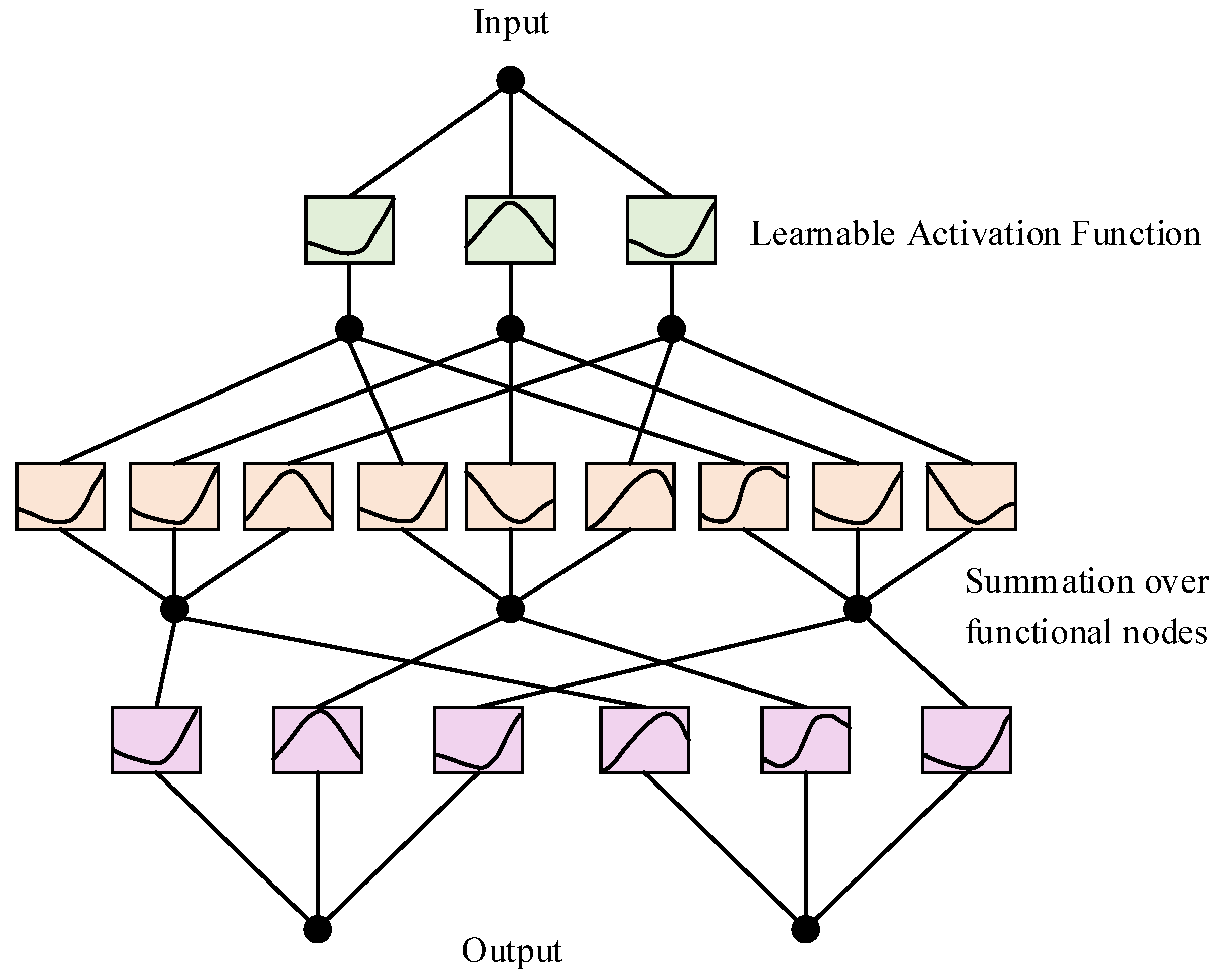
KAN (Kolmogorov–Arnold network) is a novel network architecture proposed by the MIT team in May 2024, inspired by the Kolmogorov–Arnold representation theorem [19], as illustrated in Figure 9. This theorem states that any multivariate continuous function can be decomposed into a finite sum of continuous functions of one variable and an additional continuous function. Based on this theoretical foundation, the KAN network aims to simplify the representation of complex functions, thereby improving the efficiency and interpretability of neural networks.

The architecture of KAN typically involves decomposing the input space into individual dimensions, which are then processed by one-dimensional functions before being combined. The theorem can be formally expressed as

$$f\left(x\right)={\displaystyle \sum _{q=1}^{2n+1}{\phi }_q}\left({\displaystyle \sum _{p=1}^n{\varphi }_{q,p}\left(x_p\right)}\right)$$

(4)

where $f\left(x\right)$ denotes the output of the function; the upper limit of the summation of $2n+1$ is related to the input dimension; $n$; $x_p$ represents the p-th component of the input vector $x$; where $p=1,2,\dots ,n$; ${\varphi }_{q,p}\left(x_p\right)$ denotes an internal function representing the functional composition between the q-th and p-th elements; and ${\phi }_q$ is the external function corresponding to the q-th term of the outer summation.

A single KAN layer can be viewed as a matrix of one-dimensional functions:

$$\phi =\left\{{\varphi }_{q,p}\right\},p=1,2,\dots n_{in},q=1,2,\dots n_{out}$$

(5)

when constructing deep KAN models, multiple KAN layers can be stacked. The multilayer composition relationship can be expressed as

$$\mathrm{KAN}\left(x\right)=\left({\phi }_{L-1}\circ {\phi }_{L-2}\circ \dots \circ {\phi }_1\circ {\phi }_0\right)x$$

(6)

where $\mathrm{KAN}\left(x\right)$ denotes the final output of the KAN network; ${\phi }_L$ represents the function matrix of the L-th KAN layer; and $\circ$ indicates the layer-wise functional composition or inter-layer connection.

3.4. SA Model

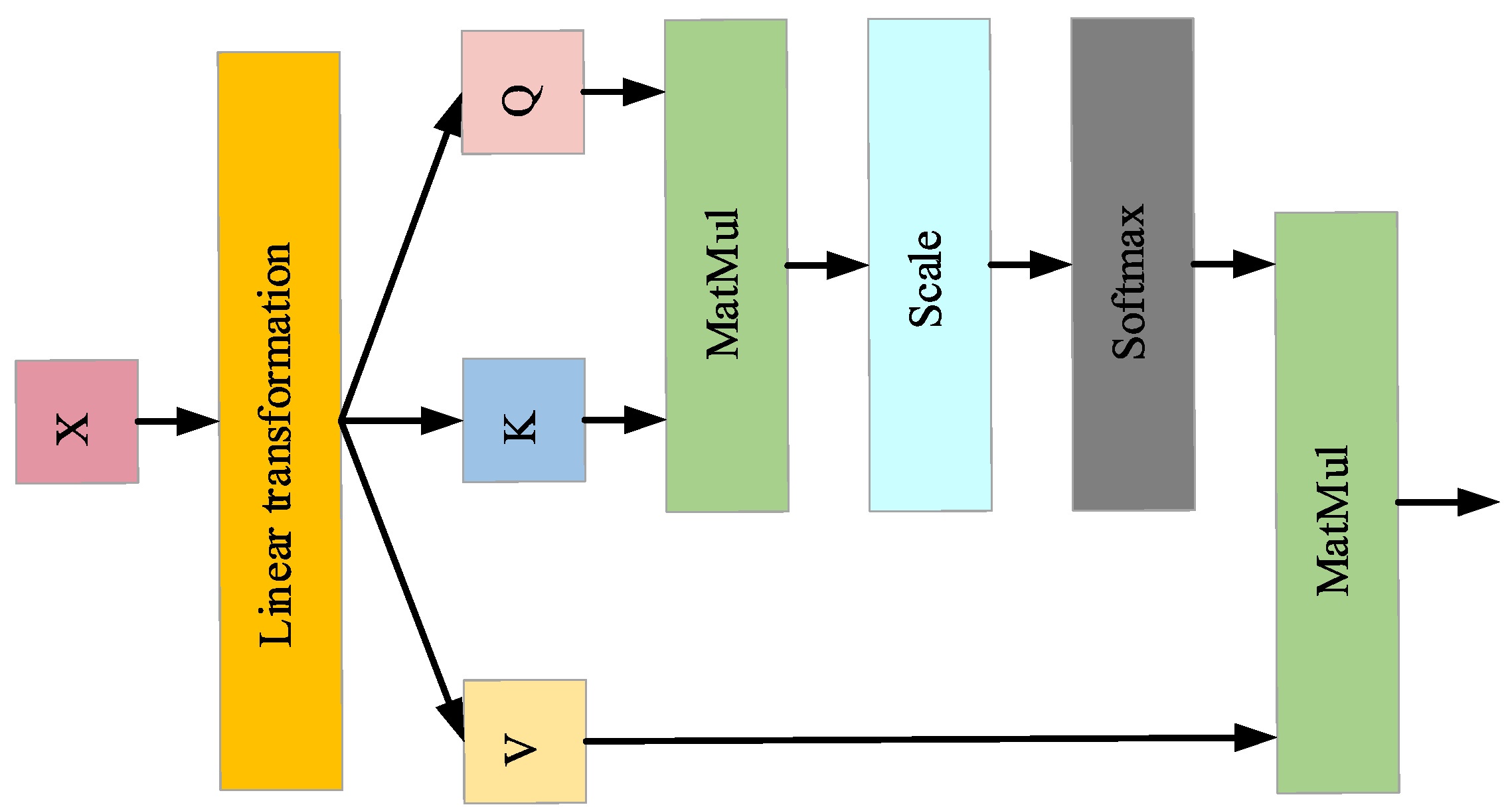
The self-attention mechanism dynamically adjusts weights to highlight important features while suppressing redundant information, enhancing the model’s ability to capture complex patterns. The architecture is shown in Figure 10. The self-attention operation is mathematically defined as follows:

$$Attention\left(Q,K,V\right)=soft\max \left({\displaystyle \frac{Q{K}^T}{\sqrt{d_k}}}\right)V$$

(7)

where $Q$, $K$, and $V$ represent the query vector, key vector, and value vector, respectively; $d_k$ denotes the dimension of the key vector $K$.

3.5. TSMixer-BiKSA Network Model Structure

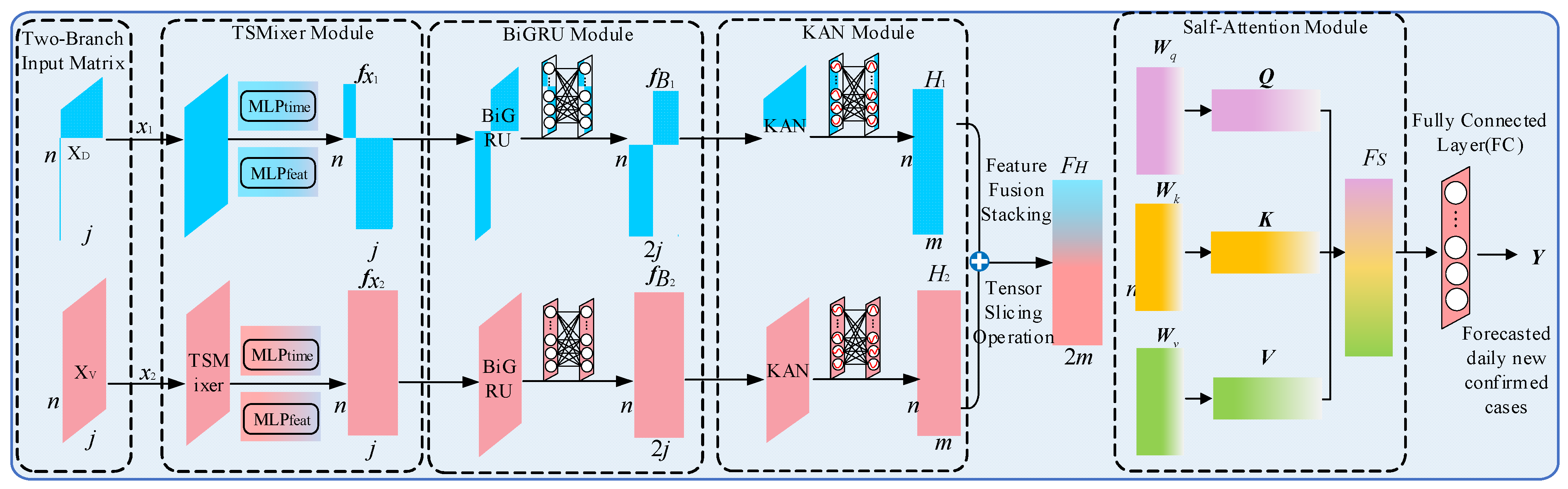
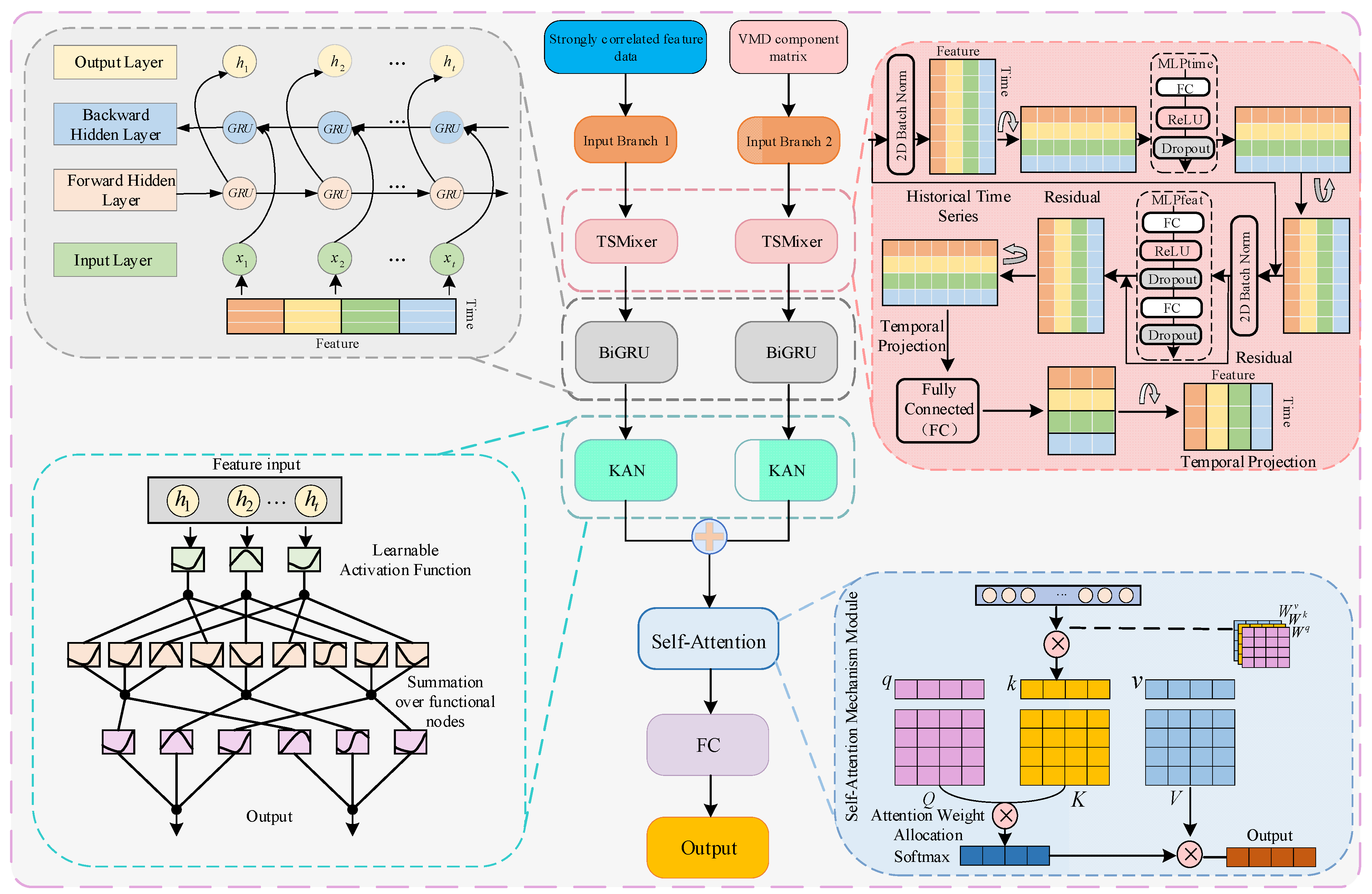
To address the feature extraction problem for daily new confirmed COVID-19 cases and their strongly correlated external factors, this study proposes a parallel dual-branch architecture. The two branches are designed to separately process the matrix of strongly correlated external variables and the VMD-decomposed component matrix of newly confirmed cases. Taking a single sample as an example, the detailed processing flow of each module is illustrated in Figure 11.

The external variable matrix (7 × 5) and the VMD-decomposed component matrix (7 × 6) are first fed into the TSMixer module for time-series modeling. To preserve information integrity, the output dimension of the temporal mapping layer matches the input, leveraging fully connected interactions across both temporal and feature dimensions. This design promotes effective feature mixing and enhances temporal dependencies and representational power.

The extracted features are then passed to a bidirectional GRU (BiGRU), which projects the low-dimensional TSMixer output into a higher-dimensional space using a large number of neurons. This enables richer bidirectional contextual modeling and improved long-term dependency capture. BiGRU also standardizes the outputs of both input branches (e.g., 7 × 128), ensuring compatibility for feature fusion.

Next, the KAN module performs hierarchical nonlinear transformations to extract high-order features. Its compact hidden dimension acts as a bottleneck (reducing the feature size to 7 × 64), balancing computational efficiency with enhanced expressiveness.

A self-attention mechanism is then applied to adaptively weight and fuse features from both branches. The fused representation is passed through a fully connected layer to produce the final output—the predicted daily new confirmed COVID-19 cases.

This multi-level feature extraction and fusion framework significantly improves the model’s predictive accuracy. Based on this architecture, we name the dual-branch prediction model the TSMixer-BiKSA network, as illustrated in Figure 12.

3.6. Forecasting Process

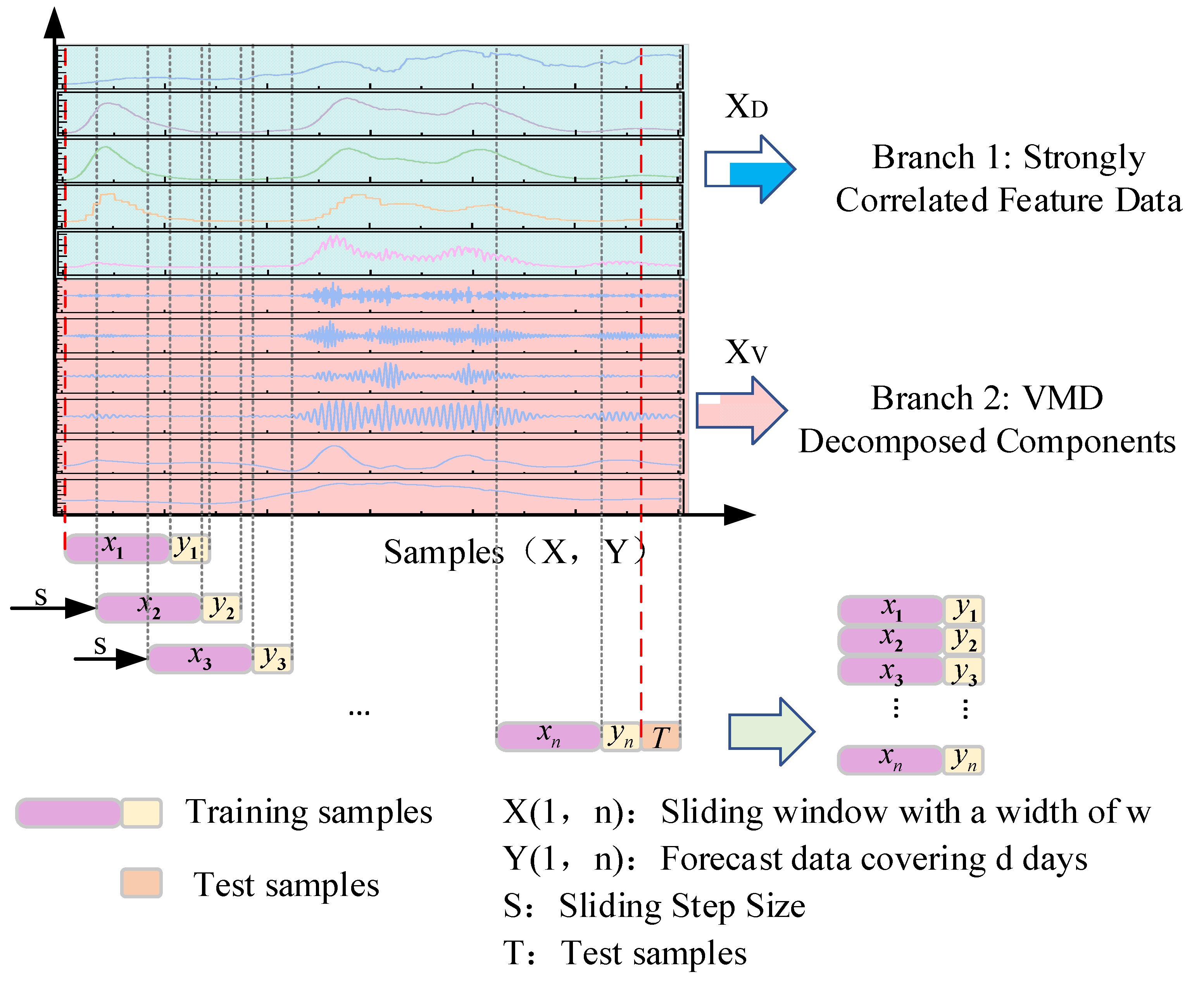
The COVID-19 trend forecasting approach proposed in this study—based on Variational Mode Decomposition (VMD) and the TSMixer-BiKSA network—consists of two main stages: data preprocessing and analysis, and model training and prediction evaluation. In the first stage, correlation analysis is conducted to identify variables that exhibit strong associations with daily new confirmed cases. These highly correlated variables are then combined with the case data to form the first input branch of the model. In parallel, the case data is decomposed using VMD, and the resulting component matrix forms the second input branch. Both branches’ data are sampled via a sliding window and then fed into the TSMixer-BiKSA deep learning model. As illustrated in Figure 13, during the model training and prediction evaluation stage, the TSMixer-BiKSA network leverages a multi-module collaborative mechanism to efficiently extract and fuse multi-scale temporal features from the daily new confirmed cases and associated factors, thereby enhancing forecasting accuracy. The process is detailed as follows:

• The TSMixer module primarily processes time-series data through two multilayer perceptron (MLP) structures: temporal mixing and feature mixing. Specifically, the temporal mixing MLP operates along the temporal dimension, independently extracting temporal dependencies for each feature channel. The computational procedure is described as follows:

  $$\left\{\begin{array}{l}{X}_1=LN\left(X\right)\hfill \\ X_T=\sigma (X_1{W}_n)\hfill \\ X_T=X+X_T\hfill \end{array}\right.$$

  (8)

  where the input matrix $X\in {ℝ}^{n\times j}$ (where n is the number of time steps and j is the feature dimension) corresponds to inputs from the two branches: X_D and X_V, respectively. $W_n\in {ℝ}^{n\times n}$ denotes the temporal mixing weights; $\sigma$ is the activation function (GELU is used in this paper); LN denotes the layer normalization function; and the residual connection symbol (+) indicates element-wise addition.
  The feature mixing MLP operates along the feature dimension, transforming the feature vector at each time step to capture intrinsic relationships among variables. The computation process is defined as follows:

  $$\left\{\begin{array}{l}{X}_2=LN\left(X_T\right)\hfill \\ X_C=\sigma (X_2{W}_j)\hfill \\ f_{xi}=X_T+X_C\hfill \end{array}\right.$$

  (9)

  where $W_j\in {ℝ}^{j\times j}$ denotes the feature mixing weights and $f_{xi}\in {ℝ}^{n\times j}\left(i=1,2\right)$ represents the output of each branch’s TSMixer module. In this study, the output of the TSMixer modules is maintained at the same dimensionality as the input.
• For the BiGRU module, an input consisting of an n × j matrix—where each row is an j-dimensional feature vector—is fed into the BiGRU. The association between historical and future data is reinforced through the principles of forward and backward propagation, facilitating the extraction of temporal features inherent in daily new confirmed cases and their associated variables at each time step. The computational procedure is detailed as follows:

  $$\left\{\begin{array}{l}\overrightarrow{{h_t}^i}={{\delta }_t}^i\left(\overrightarrow{W_{x_i}}f{H}_i+\overrightarrow{{W^i}_h}\overrightarrow{{h^i}_{t-1}}+\overrightarrow{b_i}\right)\hfill \\ \overleftarrow{{h_t}^i}={{\delta }_t}^i\left(\overleftarrow{W_{x_i}}f{H}_i+\overleftarrow{{W^i}_h}\overleftarrow{{h^i}_{t-1}}+\overleftarrow{b_i}\right)\hfill \\ f_{B_i}={{\delta }_t}^i\left(\overrightarrow{W_1}\overrightarrow{{h_t}^1}+\overleftarrow{W_i}\overleftarrow{{h_t}^i}\right)\hfill \end{array}\right.$$

  (10)

  where i = 1, 2. $\overrightarrow{W_{x_i}}$ and $\overleftarrow{W_{x_i}}$ are the weight matrices that project the input layer to the forward and backward hidden layers, respectively. $f_{x_i}$ denotes the output from the TSMixer module. $\overrightarrow{{W^i}_h}$ and $\overleftarrow{{W^i}_h}$ are the recurrent weight matrices that map the outputs from the previous time step to the current time step in the forward and backward hidden layers, respectively. $\overrightarrow{b_i}$ and $\overleftarrow{b_i}$ are the bias vectors for the forward and backward hidden layers. $\overrightarrow{W_i}$ and $\overleftarrow{W_i}$ represent the weight matrices that project the forward and backward hidden states to the output layer. ${{\delta }_t}^i$ denotes the hyperbolic tangent activation function. $\overrightarrow{{h_t}^i}$ and $\overleftarrow{{h_t}^i}$ are the forward and backward hidden states at time step t for each of the three input branches. The output of the BiGRU module is denoted as $f_{B_i}$. Assuming a batch size of h, the output of each BiGRU branch is a feature matrix of dimension h × n × 2j, meaning that, at each time step, each branch produces an output of dimension n × 2j after passing through the BiGRU module [25].
• In the first step of the KAN module, each neuron performs a linear transformation on the input feature matrix:

  $$Z=f_{B_i}\cdot W+B$$

  (11)

  where $W\in {ℝ}^{2j\times m}$ is the weight matrix that maps the output from dimension j to the hidden layer of dimension m, $B\in {ℝ}^{n\times m}$ is the bias matrix, and $Z\in {ℝ}^{n\times m}$ is the result of the linear transformation:

  $$Z_{ij}={\displaystyle \sum _{k=1}^d{x_i}^{\left(k\right)}{{\omega }_k}^{\left(j\right)}+b_j}$$

  (12)
  Unlike MLPs that use fixed activation functions such as ReLU, the KAN introduces a learnable one-dimensional nonlinear function ${\Phi }_j$ at this stage:

  $$H_{ij}={\Phi }_j\left(Z_{ij}\right)$$

  (13)
  That is, $H=\Phi \left(Z\right)$, where ${\Phi }_j\left(\cdot \right)$ is a learnable univariate function applied element-wise to each column of Z:

  $$H_{ij}={\Phi }_j\left({\displaystyle \sum _{k=1}^d{x_i}^{\left(k\right)}{{\omega }_k}^{\left(j\right)}+b_j}\right)$$

  (14)
  These learnable functions are typically parameterized by piecewise polynomials or small neural networks, rather than fixed functions like ReLU or Sigmoid. The final output of the KAN module is expressed as $H_i\in {ℝ}^{n\times m}$ [26].
• The temporal features H₁ and H₂ extracted by the KAN modules are stacked and fused to obtain the spatiotemporal feature F_H of daily new confirmed cases, with dimensions h × n × 2m. Subsequently, a self-attention mechanism is applied to associate and interact with information across different positions within the sequence, enabling comprehensive capture of dependencies and enhancing the model’s ability to identify and focus on critical information. The computational process is as follows:

  $$F_H=H_1\oplus H_2$$

  (15)

  $$\left\{\begin{array}{l}Q=F_M\times W^q\hfill \\ K=F_M\times W^k\hfill \\ V=F_M\times W^v\hfill \\ F_S=soft\max \left({\displaystyle \frac{Q\times K^T}{\sqrt{d_k}}}\right)V\hfill \end{array}\right.$$

  (16)

  where “⊕” denotes the concatenation of features from the two branches; F_H represents the resulting one-dimensional long vector after stacking and fusion; W^q, W^k, and W^v are the query, key, and value weight matrices in the self-attention (SA) module, respectively; Q, K, and V denote the corresponding query, key, and value matrices; softmax is the normalization function; T indicates the matrix transpose operation; d_k is the scaling factor for normalization; and F_S represents the output feature sequence from the self-attention module.
• The spatiotemporal feature sequence F_S output by the attention mechanism is then tensor-sliced to extract the features at the final time step (with dimensions h × 2m), which are subsequently fed into a fully connected layer to generate the predicted daily new confirmed COVID-19 cases Y for each time step.

Figure 13. Framework of the prediction process.

Figure 13. Framework of the prediction process.

4. Experiments and Results Analysis

All experiments were conducted on hardware consisting of an Intel Core i5-13400F CPU (2.5 GHz), 64 GB RAM, and an NVIDIA RTX 3060 GPU (12 GB). Models were developed using PyTorch 1.10.1 within PyCharm 2024.1.1. Training employed the Adam optimizer with a learning rate of 0.001, batch size of 16, and up to 500 epochs.

To objectively evaluate performance, root mean square error (RMSE), mean absolute error (MAE), mean absolute percentage error (MAPE), and coefficient of determination (R²) were used. The calculation formulas are as follows:

$$e_{RMSE}=\sqrt{{\displaystyle \frac{1}{n}}{\displaystyle \sum _{i=1}^n{\left({\widehat{y}}_i-y_i\right)}^2}}$$

(17)

$$e_{MAE}={\displaystyle \frac{1}{n}}{\displaystyle \sum _{i=1}^n\left|{\widehat{y}}_i-y_i\right|}$$

(18)

$$e_{MAPE}={\displaystyle \frac{1}{n}}{\displaystyle \sum _{i=1}^n\left|\frac{{\widehat{y}}_i-y_i}{y_i}\right|}\times 100\%$$

(19)

$$R^2=1-{\displaystyle \frac{{\displaystyle \sum _{i=1}^n{\left(y_i-{\widehat{y}}_i\right)}^2}}{{\displaystyle \sum _{i=1}^n{\left(y_i-{\overline{y}}_i\right)}^2}}}$$

(20)

where ${\widehat{y}}_i$ denotes the predicted value of daily new confirmed cases; $y_i$ denotes the actual value of daily new confirmed cases; ${\overline{y}}_i$ represents the mean of the actual daily new confirmed cases.

4.1. Model Parameter Settings

• Model Architecture and Parameter Settings

The hidden layer dimension of the TSMixer module significantly influences its capability to capture temporal and variable features, thereby affecting the BiGRU’s ability to extract deep correlations within the feature matrix. The number of neurons in the BiGRU must balance modeling bidirectional long- and short-term dependencies with computational efficiency to ensure accurate predictions while preventing overfitting and resource wastage. Similarly, the hidden layer size of the KAN module directly impacts its capacity to extract higher-order features.

Based on these considerations, this study conducts comparative experiments to jointly evaluate the effects of varying the TSMixer hidden layer dimensions, BiGRU neuron counts, and KAN hidden layer sizes. Optimal parameter configurations for each module are determined from the experimental results.

Table 2. Comparison of experimental errors across different model parameters.

Serial Number	TSMixer Module	BiGRU Module	KAN Module	Evaluation Metrics
				eRMSE	eMAE	eMAPE/%
A1	16	64	64	140.074	101.61	0.905
A0	32	64	64	139.984	93.245	0.712
A2	64	64	64	267.582	208.573	2.539
A3	32	32	64	322.344	285.048	2.825
A4	32	128	64	167.778	117.264	0.869
A5	32	64	32	177.575	122.564	0.767
A6	32	64	128	202.147	143.728	1.591

presents the evaluation metrics and prediction errors under a 7-day sliding window with single-step forecasting.

As presented in Table 2, the proposed MB-TSMixer-BiKSA network model achieves the lowest prediction errors and optimal forecasting performance when the TSMixer hidden layer dimension is set to 32, and both the BiGRU neuron count and KAN hidden layer dimension are 64. This result suggests that this specific parameter configuration enables the model to maximize its overall feature extraction capability and attain the most effective parameter setting.

2.

Model Training Hyperparameter Settings

Hyperparameters play a crucial role in determining the training effectiveness and overall performance of the model, with varying combinations resulting in differences in accuracy and convergence speed. Comparative experiments enable a systematic assessment of the strengths and weaknesses of different hyperparameter settings, facilitating intuitive performance comparisons across configurations. This approach allows for the precise identification of optimal hyperparameters tailored to specific tasks and datasets, thereby ensuring the model’s accuracy and stability.

Table 3. Error comparison across different hyperparameter configurations.

Epoch	Batch	Learning Rate	Time	Metric
				eRMSE	eMAE	eMAPE/%	R2
300	8	0.001	149 s	164.217	111.756	0.916	0.998
300	16	0.001	73 s	185.498	132.325	0.834	0.998
300	16	0.0001	74 s	448.317	381.568	3.255	0.992
500	16	0.001	125 s	139.984	93.245	0.712	0.999
500	32	0.001	65 s	154.415	108.062	0.814	0.999

presents the experimental outcomes under the optimal model parameters with various training hyperparameters, while Figure 14 illustrates the corresponding training loss curves.

The experimental results indicate that moderately increasing the number of training epochs substantially enhances model performance. In particular, the configuration with a batch size of 16 and a learning rate of 0.001 achieves the best balance between error and goodness of fit, attaining the lowest RMSE (139.984) and highest R² (0.999), while requiring only 125 s of training time. This setup effectively balances training efficiency and predictive accuracy. Conversely, excessively large batch sizes or very small learning rates result in performance deterioration. Overall, the combination of 500 epochs, batch size 16, and learning rate 0.001 demonstrates the most optimal and stable performance, representing a favorable trade-off between training speed and model accuracy.

4.2. Decomposition Comparative Experiments

To evaluate the performance advantage of the proposed dual-branch input strategy based on VMD-decomposed features, we designed the following input configurations for comparative experiments:

Input 1: Single-feature, single-branch input using only daily new confirmed cases;

Input 2: Multi-feature, single-branch input using daily new confirmed cases;

Input 3: ICEEMDAN-based multi-feature, dual-branch input;

Input 4: EWT-based multi-feature, dual-branch input;

Proposed Approach: VMD-based multi-feature, dual-branch input.

All comparative experiments were conducted using 3-day and 7-day sliding windows over a 200-day test set, with one-, two-, and three-step-ahead predictions (1 day per step). To mitigate the impact of random fluctuations, each experiment was repeated 10 times, and the average prediction value across the 10 runs was taken as the final result.

Table 4. Prediction errors of different decomposition methods.

Window Size	Input Scheme	eRMSE			eMAE			eMAPE/%			R2
		1-Step	2-Step	3-Step	1-Step	2-Step	3-Step	1-Step	2-Step	3-Step	1-Step	2-Step	3-Step
3 d	Input1	1974.616	2651.935	2986.401	1184.059	1651.305	1996.193	7.611	12.080	16.784	0.851	0.746	0.679
	Input2	1787.724	2364.163	2551.460	1153.233	1491.883	1629.628	8.097	9.859	11.336	0.878	0.798	0.765
	Input3	931.628	1227.512	1476.610	730.476	912.099	1141.951	6.474	7.429	9.486	0.967	0.946	0.921
	Input4	712.712	1192.767	1461.539	568.241	901.788	1217.332	3.829	5.602	10.382	0.981	0.949	0.923
	Proposed Approach	279.292	716.258	964.163	205.716	529.424	723.717	1.443	3.417	5.227	0.997	0.981	0.967
7 d	Input1	2083.698	2387.521	2925.710	1675.953	1892.179	2377.007	12.492	16.554	22.251	0.834	0.794	0.674
	Input2	1720.037	2280.838	2426.458	1288.614	1736.173	1729.666	9.818	12.569	12.159	0.887	0.812	0.775
	Input3	1005.259	1070.169	1697.9766	683.561	772.924	1282.453	4.915	7.522	13.546	0.961	0.959	0.890
	Input4	594.201	1103.042	2042.177	443.101	824.774	1620.116	2.582	5.340	12.765	0.986	0.956	0.841
	Proposed Approach	139.984	448.579	767.135	93.245	313.176	556.106	0.712	2.609	3.976	0.999	0.993	0.978

presents a comparison of prediction errors on the test set for all configurations, while Figure 15 illustrates the fitting performance and error analysis of the predicted results for each experimental group.

The following is shown in Table 4 and Figure 15:

(1) The introduction of multi-feature input significantly improves the model’s predictive performance across different forecasting horizons. Taking the three-step prediction under a 3-day window as an example, the e_RMSE decreases from 2986.401 to 2551.460, a reduction of approximately 14.6%; the e_MAE decreases from 1996.193 to 1629.628, a reduction of about 18.3%; the e_MAPE decreases from 16.784% to 11.336%, a reduction of approximately 32.5%; and the R² increases from 0.679 to 0.765, indicating a significant improvement in the coefficient of determination. Under a 7-day window, the three-step prediction e_RMSE decreases from 2925.710 to 2426.458, representing a reduction of around 17.1%. Overall, multi-feature input effectively enhances the model’s ability to characterize complex data patterns by incorporating additional dimensions of temporal information, which is especially advantageous in multi-step forecasting tasks by alleviating error accumulation and improving model stability.

(2) When combining VMD decomposition with multi-feature input, the model outperforms other decomposition methods such as ICEEMDAN and EWT on all evaluation metrics. For example, under the 7-day window for three-step prediction, the proposed method achieves an e_RMSE of 767.135, which represents reductions of approximately 54.8% and 62.4% compared to ICEEMDAN (1697.976) and EWT (2042.177), respectively. The e_MAPE decreases from 13.546% (ICEEMDAN) and 12.765% (EWT) to 3.976%, with reductions of 70.6% and 68.8%, respectively. The R² is significantly improved from 0.890 (ICEEMDAN) and 0.841 (EWT) to 0.978. Analysis of the normal distribution of prediction errors across different forecasting steps reveals that the proposed input scheme achieves the lowest mean and standard deviation of errors, indicating superior model stability and reliability. These findings highlight VMD’s enhanced feature extraction and noise reduction capabilities. When combined with multi-feature input, VMD effectively captures essential temporal information, markedly improving the model’s stability and accuracy in multi-step forecasting tasks.

(3) Under the same modeling approach, extending the input window length significantly improves overall performance in multi-step forecasting tasks. Taking the proposed method as an example, for three-step prediction, the e_RMSE under the 7-day window is 767.135, approximately 20.4% lower than that of the 3-day window (964.163); the e_MAPE decreases from 5.227% to 3.976%, a relative reduction of about 23.9%; and the R² increases from 0.967 to 0.978, further enhancing fitting performance. This indicates that appropriately extending the input window provides the model with more comprehensive temporal context, which helps to better capture long-term trends and periodic fluctuations, thereby improving prediction stability. Additionally, introducing multi-step prediction mechanisms (e.g., two-step, three-step) not only expands the model’s application scope but also strengthens its ability to perform continuous forecasts over multiple future days, demonstrating robustness and practical value when handling highly uncertain temporal tasks.

4.3. Model Comparison Experiments

To validate the superiority of the proposed TSMixer-BiKSA network model in forecasting COVID-19 epidemic trends, ablation experiments were designed. The subcomponent matrices obtained from VMD decomposition and the strongly correlated factor variable matrices were separately fed into the following ablation models:

Experiment B1: TSMixer-KAN;

Experiment B2: BiGRU-KAN;

Experiment B3: TSMixer-BiGRU;

Experiment B0: Proposed full model.

The models from each ablation experiment group were evaluated under different sliding window sizes and forecasting horizons. The prediction results are presented in

Table 5. Comparison of experimental errors across different prediction models.

Window Size	Model	eRMSE			eMAE			eMAPE/%			R2
		1-Step	2-Step	3-Step	1-Step	2-Step	3-Step	1-Step	2-Step	3-Step	1-Step	2-Step	3-Step
3 d	TSMixer-KAN	812.370	1028.737	1770.2	481.574	722.555	1343.136	2.892	5.902	12.245	0.975	0.962	0.887
	BiGRU-KAN	355.039	726.022	1038.624	286.737	531.972	744.122	2.339	3.621	5.31	0.995	0.978	0.956
	TSMixer-BiGRU	301.399	943.671	1157.183	228.326	569.986	931.261	2.272	4.198	6.372	0.996	0.97	0.952
	Proposed Model	279.292	716.258	964.163	205.716	529.424	723.717	1.443	3.417	5.227	0.997	0.981	0.967
7 d	TSMixer-KAN	666.847	1009.587	1077.309	385.019	709.559	861.7662	2.534	5.145	4.899	0.983	0.963	0.962
	BiGRU-KAN	228.197	470.823	1017.612	203.928	380.896	708.452	1.884	2.812	4.885	0.998	0.991	0.963
	TSMixer-BiGRU	250.412	741.062	974.072	204.84	647.088	758.214	1.226	6.249	4.969	0.997	0.98	0.964
	Proposed Model	139.984	448.579	767.135	93.245	313.176	556.106	0.712	2.609	3.976	0.999	0.993	0.978

and Figure 16.

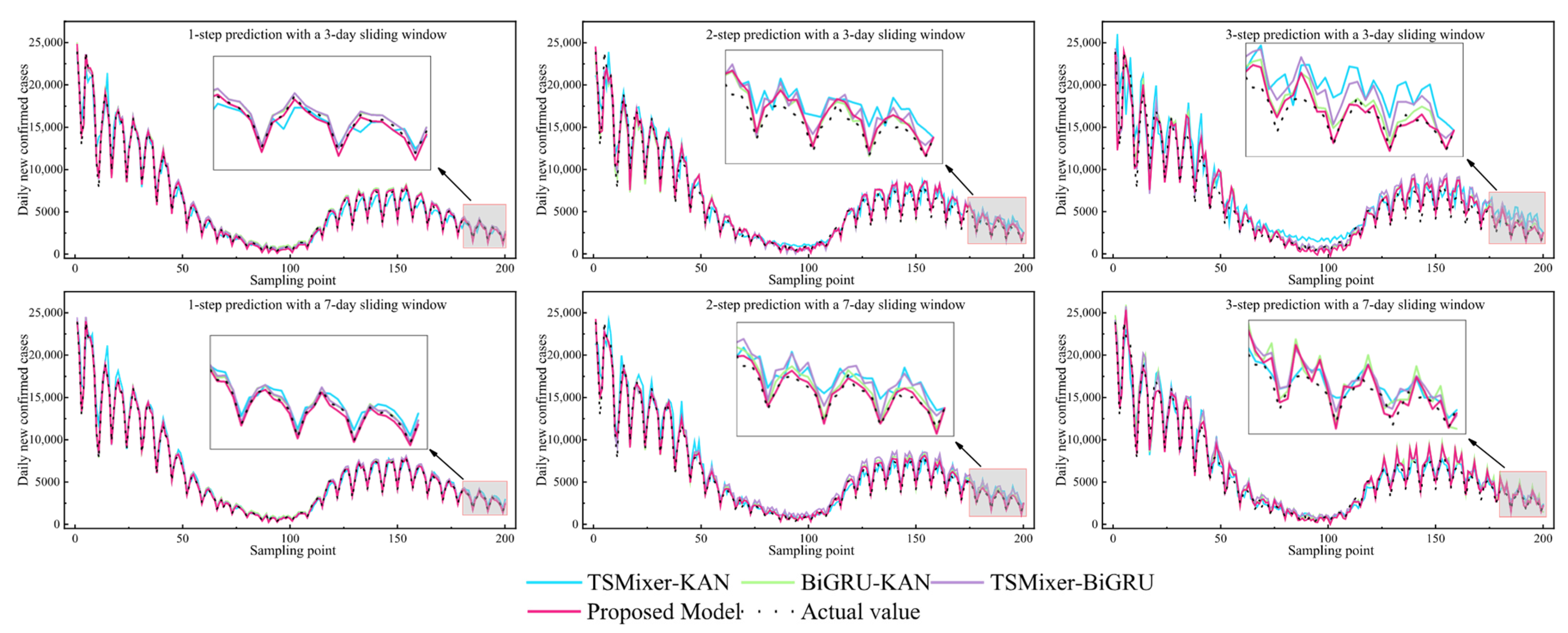
As shown in Table 5 and Figure 16, the proposed model consistently demonstrates optimal performance across different window sizes and forecasting horizons. For instance, in the 7-day window with three-step prediction, the proposed model achieves an e_RMSE of 767.135, representing reductions of 28.8%, 24.6%, and 21.3% compared to TSMixer-KAN, BiGRU-KAN, and TSMixer-BiGRU, respectively. The e_MAPE is 3.976%, significantly lower than the 4.899%, 4.885%, and 4.969% observed in the other model combinations. The R² reaches 0.978, markedly outperforming the other models. This trend is similarly evident under the 3-day window, indicating that the synergistic integration of the modules effectively enhances the model’s nonlinear modeling capacity and temporal feature extraction ability.

Specifically, the TSMixer module leverages a fully connected structure to model interactions along both the temporal and feature dimensions, improving the mixed representation of temporal features; the BiGRU module models temporal dependencies, strengthening trend capturing; and the KAN module, through adaptive kernel mapping, enhances nonlinear modeling capacity, improving adaptability to complex nonlinear feature variations. Collectively, TSMixer-BiKSANet integrates the strengths of these components to achieve efficient feature extraction, thereby improving prediction accuracy while optimizing computational efficiency.

Table 6. Performance metrics of models in ablation experiments.

Model	Number of Parameters	FLOPs (Floating Point Operations)	Total Training Time	Average Time per Batch	Samples Processed per Second
TSMixer-KAN	115,034	5,976,064	45 s	0.0066 s	995,636
BiGRU-KAN	268,417	19,300,352	52 s	0.0083 s	790,535
TSMixer-BiGRU	254,298	16,678,912	39 s	0.0064 s	1,030,415
Proposed Model	270,170	23,023,616	63 s	0.0093 s	705,024

presents the performance of the model under different ablation experiment configurations. Experiment B1 employs the relatively simple TSMixer-KAN model, which features a lower parameter count and computational complexity, resulting in higher training efficiency but limited feature extraction capability and consequently lower prediction accuracy. Experiment B2 introduces the BiGRU module, significantly enhancing temporal feature modeling and improving prediction accuracy; however, this comes at the cost of increased model parameters and computational complexity, leading to a decrease in training efficiency. Experiment B3 combines TSMixer with BiGRU while removing the KAN module, slightly reducing the parameter count but yielding limited performance gains, especially showing decreased prediction accuracy under a 7-day sliding window. Experiment B0 corresponds to the full proposed model, integrating the advantages of TSMixer, BiGRU, and KAN modules. Although this configuration increases model complexity and training time, it achieves the best prediction accuracy across all window sizes, demonstrating a significant performance advantage.

Considering that the differences in training time among the models are marginal and the increase in complexity remains within an acceptable range, this study achieves a reasonable balance between accuracy and efficiency through multi-module collaborative design, showcasing an effective strategy for performance improvement.

Table 7. Paired sample t-test results of prediction errors for different model schemes.

Window Size		3-Day Window				7-Day Window
Experimental Comparison		B1-B2	B1-B3	B2-B3	B3-B0	B1-B2	B1-B3	B2-B3	B3-B0
1-step	t-statistic value	−5.9225	−4.5024	6.5021	16.3134	0.7449	0.8779	0.5965	17.8022
	p-value (<0.05)	<0.0001	<0.0001	<0.0001	<0.0001	0.4572	0.3810	0.5515	<0.0001
2-step	t-statistic value	3.7640	1.5818	−8.0871	1.6208	2.5550	−2.0835	−17.9341	14.6343
	p-value (<0.05)	0.0002	0.0115	<0.0001	0.0106	0.0114	0.0385	<0.0001	<0.0001
3-step	t-statistic value	5.3163	2.7711	−5.9566	7.2136	−4.3465	−7.4297	−5.2316	12.6862
	p-value (<0.05)	<0.0001	0.0061	<0.0001	<0.0001	<0.0001	<0.0001	<0.0001	<0.0001

presents the results of paired sample t-tests on the prediction errors of daily new confirmed COVID-19 cases under sliding window widths of 3 days and 7 days across different model configurations. The results indicate that the integration of TSMixer and KAN (B1 vs. B3) significantly improves the multi-step forecasting performance, with predictions under the 7-day sliding window exhibiting greater stability, demonstrating the effectiveness of KAN in enhancing temporal feature modeling. The introduction of the BiGRU structure (B1 vs. B2) also yields significant performance improvements at all time points, validating the importance of sequential contextual information for prediction. The combination of TSMixer and BiGRU (B2 vs. B3) shows significant advantages at all time steps, highlighting their synergistic role in performance enhancement.

Notably, in the single-step forecasting task with a 7-day window, the t-test p-values for comparisons B1 vs. B2, B1 vs. B3, and B2 vs. B3 are all greater than 0.05, indicating no statistically significant differences among these models. This may be attributed to the 7-day window providing sufficient temporal information, allowing baseline models to perform well in single-step prediction with limited differences. Upon further incorporating the self-attention mechanism into B3 (B3 vs. B0), the proposed model achieves statistically significant performance improvements at most time points, especially at t = 1 and t = 2, reflecting its enhanced ability to capture critical features at key time steps. However, minor fluctuations at a few time points suggest that the application of attention mechanisms may require task-specific adjustments.

In summary, the experimental results validate the effectiveness and robustness of the module combinations in improving prediction performance, while revealing subtle yet meaningful differences among the models.

4.4. Comparison Experiments with Existing Methods

To comprehensively evaluate the performance of the proposed model in practical forecasting tasks, we selected several standard baseline models, including LSTM [26], ARIMA [15], and Transformer [27], as well as representative hybrid forecasting approaches from the existing literature: CNN-LSTM-ARIMA, TCN-LSTM-ARIMA, SSA-LSTM-ARIMA [15], and pop LSTM [28]. All models were tested on the same dataset under identical conditions. 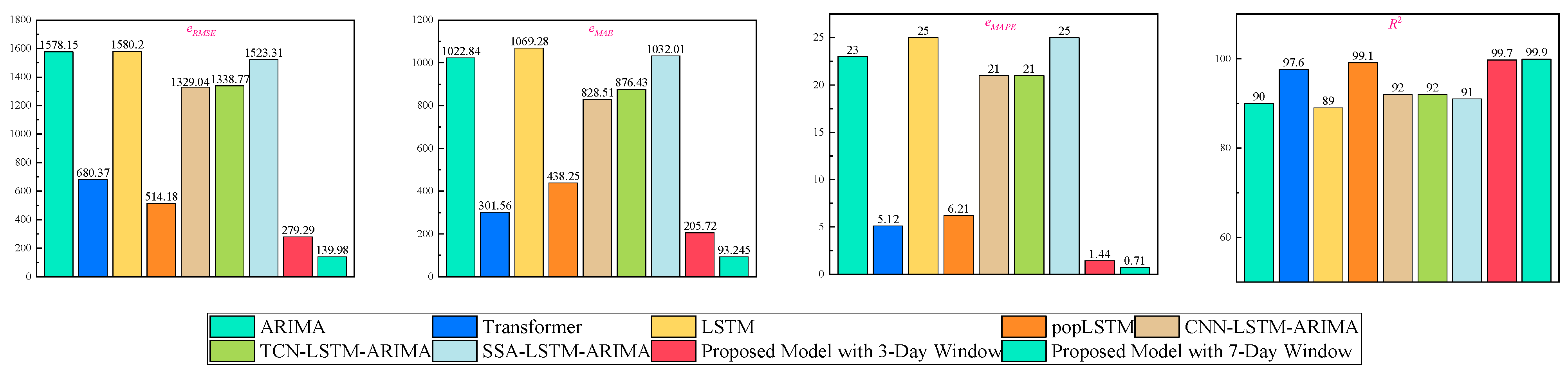The comparative results are presented in Figure 17.

The comparative results demonstrate that the proposed hybrid architecture significantly outperforms all baseline and reference models across multiple evaluation metrics. Under the 3-day forecasting window, the model achieves an e_RMSE of 279.29, an MAE of 205.72, and an exceptionally low e_MAPE of 1.44%, with an R² score reaching 99.7%. These results indicate a superior predictive accuracy and fitting capability compared to the existing mainstream models. For instance, compared with the well-performing Transformer model, the proposed model reduces e_RMSE by 59% and e_MAE by 31.7%, and it lowers e_MAPE from 5.12% to 1.44%, marking a substantial reduction in relative error. Simultaneously, the R² improves from 97.6% to 99.7%, indicating an enhanced capacity to capture temporal trends. When compared with the improved pop LSTM model, which already achieves a high R² of 99.1%, the proposed model still yields a better performance across all error metrics: e_RMSE decreases from 514.18 to 279.29, and e_MAPE drops from 6.21% to 1.44%, indicating a marked improvement in overall predictive precision.

Regarding the commonly used hybrid models in the literature—such as CNN-LSTM-ARIMA, TCN-LSTM-ARIMA, and SSA-LSTM-ARIMA—although these methods enhance the fitting ability of individual models to some extent, their overall performance remains inferior. For example, the SSA-LSTM-ARIMA model records an e_MAPE of 25% and an R² of only 91%, while the proposed model reduces the e_MAPE to 1.44%, reflecting a significant improvement in accuracy and highlighting the limitations of conventional hybrid models in terms of feature extraction and modeling efficiency. Furthermore, when extending the forecasting window to 7 days, the proposed model continues to demonstrate outstanding stability and predictive performance, achieving an e_RMSE of 139.98, e_MAE of 93.25, e_MAPE of 0.71%, and R² of 99.9%. These results confirm the model’s robustness and strong generalization ability in longer-term forecasting scenarios.

In summary, the proposed hybrid architecture consistently delivers the best performance across a comprehensive set of baseline and literature-based models. It significantly enhances time-series forecasting in terms of accuracy, fit, and stability, demonstrating strong practical applicability and potential for broader adoption.

4.5. Transfer Learning

Transfer learning is a machine-learning strategy that improves the performance of models in a target domain by leveraging knowledge learned from a source domain, especially effective when the data distributions in the source and target domains are similar. Its core advantage lies in utilizing existing training experience to reduce the reliance on large amounts of labeled data in the target domain, thereby enhancing the model’s generalization ability in new environments.

To evaluate the transferability of the proposed model in COVID-19 epidemic forecasting tasks across different regions, particularly its practicality and stability in multi-step forecasting scenarios, cross-regional transfer experiments were conducted. Specifically, the model was first trained and its parameters saved based on Italy’s COVID-19 data from 21 February 2020, to 26 March 2021 (a total of 400 days). The pretrained model was then transferred to the US data for prediction validation. The US dataset was split into a training set from 21 February 2020, to 26 March 2021 (400 days) and a test set from 27 March to 12 October 2021 (200 days).

To comprehensively assess the transfer effect, the transferred model was compared against a baseline model of the same architecture but without pretraining on the Italian dataset. Experiments were conducted under various combinations of sliding window sizes (3-day, 7-day) and forecasting horizons (one-step, two-step, three-step). Figure 18 presents the results of these experiments, visually demonstrating the practical value and GitHub stability of transfer learning in cross-regional epidemic forecasting.

The experimental results demonstrate that the model maintains a strong predictive performance even without retraining on US data, indicating an excellent generalization capability. In the 3-day window forecasting task, the model achieves an e_RMSE of 5793.652, e_MAE of 3689.594, e_MAPE of 1.949%, and R² of 0.991 in the 1-step prediction, reflecting its outstanding short-term forecasting ability. Although prediction errors slightly increase with longer forecasting horizons, the R² consistently remains above 0.945, suggesting a stable trend-fitting performance.

In the 7-day window forecasting task, the 1-step prediction yields an even lower e_RMSE of 5008.489 and a higher R² of 0.994, further verifying the model’s adaptability and accuracy in medium-term forecasting. Even under the more challenging three-step prediction, e_MAPE remains below 5%, and R² stays above 0.944, indicating the model’s strong performance in capturing long-term epidemic trends.

Moreover, a comparison between predicted and actual values reveals that the prediction curves generated using transfer learning better follow the actual fluctuation patterns. Across different window sizes and forecasting steps, the model reliably predicts daily new confirmed COVID-19 cases in the US Notably, the prediction of peak and trough positions exhibits significantly improved accuracy, indicating that the pretrained knowledge transferred from the source domain effectively adapts to the data distribution of the new task. This enhances both the robustness and generalization ability of the model and leads to more accurate forecasting outcomes.

In summary, the proposed model demonstrates strong robustness, controllable prediction errors, and excellent trend-fitting capability in cross-regional transfer tasks, confirming its high practicality and broad applicability.

5. Conclusions and Future Work

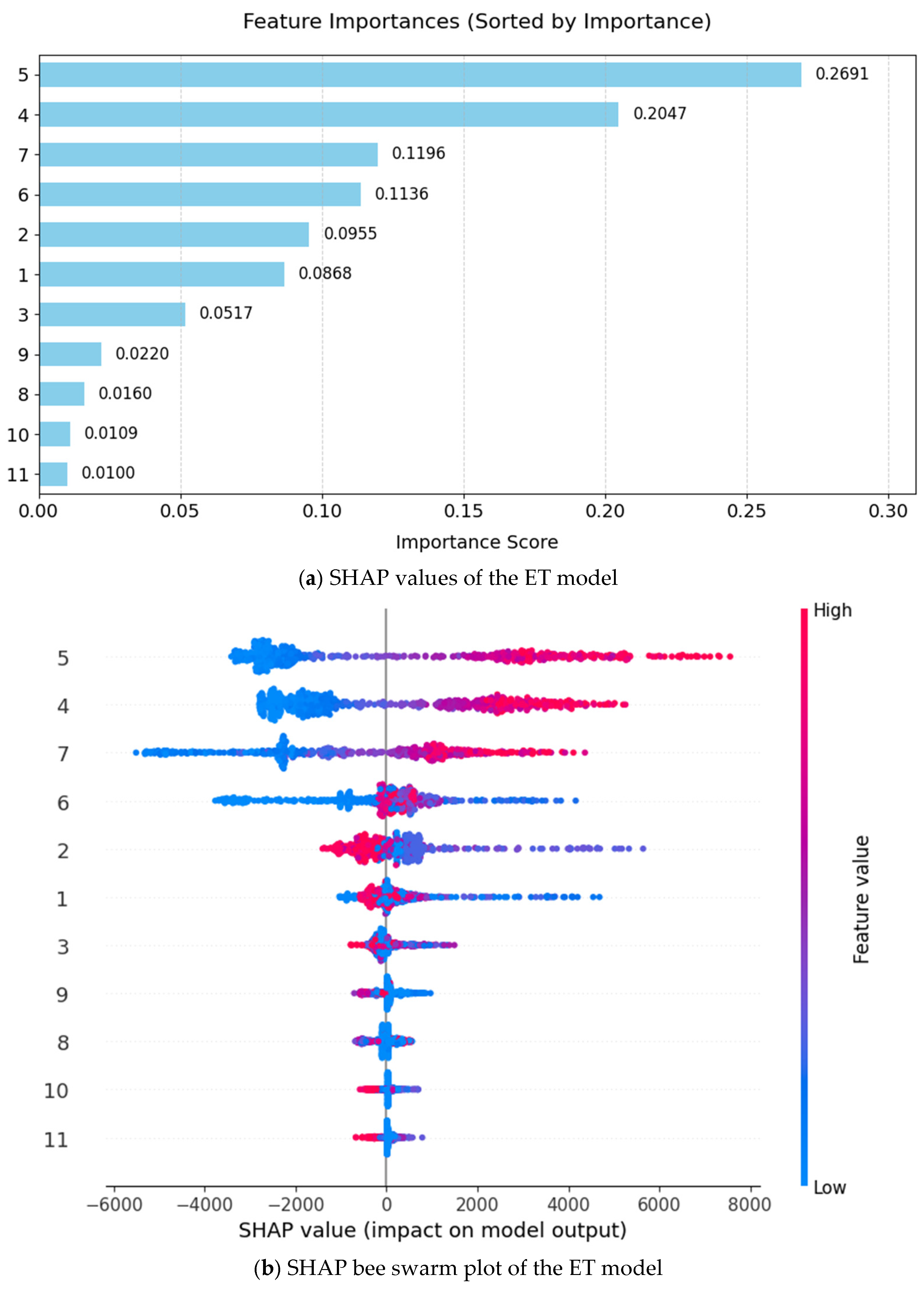
(1) By calculating both Pearson and Spearman correlation coefficients, external variables that exhibit strong positive correlations with the daily number of newly confirmed COVID-19 cases were identified. These variables, together with the case counts, were used to construct a multi-feature time-series matrix. Experimental comparisons show that, compared to using a single feature (i.e., daily new confirmed cases) as input, incorporating multiple features introduces additional dimensions of temporal information, significantly enhancing the model’s ability to capture complex data patterns. This advantage is particularly evident in multi-step forecasting tasks, where it helps to mitigate error accumulation and improves the stability of predictions. However, it is important to note that some of these external variables may have a degree of causal relationship with the case numbers. While using historical data to predict future trends can improve forecasting accuracy, in the early stages of an outbreak, the scarcity of historical data may substantially constrain model performance.

(2) The Variational Mode Decomposition (VMD) algorithm was employed to decompose the daily new case time series into multiple intrinsic mode functions with distinct fluctuation characteristics. This reduced the sequence complexity and enhanced the model’s capacity to represent temporal mappings. VMD, which decomposes signals into limited-bandwidth components within a variational framework, showed superior adaptiveness and robustness. Among the various decomposition strategies tested, the combination of VMD with multi-feature input yielded the best performance across all error evaluation metrics, validating its applicability and effectiveness in COVID-19 trend forecasting.

(3) The proposed TSMixer-BiKSA network model innovatively integrates deep temporal features of strongly correlated variables with multi-scale features from VMD-decomposed COVID-19 case series through a dual-branch parallel input architecture. The model first uses TSMixer to capture dependencies along both temporal and feature dimensions, facilitating efficient feature transformation and enhancing the representation of case trends. Subsequently, the BiGRU module captures bidirectional dependencies, improving long-term dependency learning. The KAN module extracts high-order nonlinear features, increasing adaptability to complex case fluctuations. Finally, a self-attention mechanism (SA) adaptively weights and fuses features, optimizing information integration and prediction stability. The experimental results show that the proposed model achieves the best performance across all error metrics in 1- to three-step forecasting tasks, with significantly improved R² values, validating its high predictive accuracy and excellent generalization capability in COVID-19 trend forecasting.

(4) In this study, VMD was applied by first decomposing the training set separately, and then recomputing decomposition over the full dataset (training + test set) to avoid direct information leakage from test data into the training decomposition results. However, because the training set was decomposed as a whole, some degree of future information leakage remains [29]. While full-dataset decomposition mitigates endpoint effects in the test set, it introduces boundary issues due to shared decomposition across time. Moreover, decomposing datasets of different lengths (training set vs. full set) may lead to inconsistencies in decomposition granularity. This remains a limitation and warrants further refinement in future studies.

(5) Although the KAN architecture demonstrates unique advantages in function representation, it is important to note that this approach is still in its early research stage. Having been proposed only recently, it currently lacks an extensive literature and real-world applications. Most existing studies are limited to preprint platforms, with few large-scale experimental validations or widespread industry adoption. Therefore, its performance and stability should be approached with caution in practical applications. KAN should be regarded as a promising but still emerging method that requires further evaluation.

(6) With the continuous integration of signal processing and deep learning technologies, the proposed epidemic forecasting approach—based on multi-feature input, VMD decomposition, and deep fusion—still has room for optimization. Future improvements could focus on the following:

① Introducing more advanced signal decomposition algorithms to enhance feature extraction precision and robustness;

② Incorporating deep reinforcement learning mechanisms to enable the dynamic and adaptive optimization of model parameters;

③ Extending the methodology to forecasting trends of other infectious diseases, thereby enhancing its generalizability and adaptability.

Such developments will not only further improve the predictive performance but will also reinforce the model’s practical value in epidemiological forecasting, offering more reliable technical support for global public health decision-making.