Machine Learning Techniques for Uncertainty Estimation in Dynamic Aperture Prediction

Abstract

The dynamic aperture is an essential concept in circular particle accelerators, providing the extent of the phase space region where particle motion remains stable over multiple turns. The accurate prediction of the dynamic aperture is key to optimising performance in accelerators such as the CERN Large Hadron Collider and is crucial for designing future accelerators like the CERN Future Circular Hadron Collider. Traditional methods for computing the dynamic aperture are computationally demanding and involve extensive numerical simulations with numerous initial phase space conditions. In our recent work, we have devised surrogate models to predict the dynamic aperture boundary both efficiently and accurately. These models have been further refined by incorporating them into a novel active learning framework. This framework enhances performance through continual retraining and intelligent data generation based on informed sampling driven by error estimation. A critical attribute of this framework is the precise estimation of uncertainty in dynamic aperture predictions. In this study, we investigate various machine learning techniques for uncertainty estimation, including Monte Carlo dropout, bootstrap methods, and aleatory uncertainty quantification. We evaluated these approaches to determine the most effective method for reliable uncertainty estimation in dynamic aperture predictions using machine learning techniques.

1. Introduction

The dynamic aperture (DA) is a critical parameter in the design and operational optimisation of modern circular particle accelerators. The DA is the extent of the region in phase space where particle motion remains bounded over a defined number of turns (see, e.g., [1] and references therein). The DA provides crucial insight into the non-linear beam dynamics and the mechanisms induced by non-linear resonances that lead to beam losses and reduced beam lifetime. The time evolution of DA can then be directly linked to beam losses caused by non-linear effects [2], a connection that supports the recent method for measuring DA in circular rings [3]. Furthermore, these models have been extended to the description of the time evolution of instantaneous luminosity in a circular hadron collider, when non-linear effects are included [4]. The study of DA is particularly relevant for optimising beam lifetime and, in general, performance in existing accelerators, such as the CERN Large Hadron Collider (LHC) [5], by probing multiple combinations of ring configurations to determine the best one, which will then be used in operation. Furthermore, DA is also extremely helpful in guiding the development of both significant upgrades, such as the High-Luminosity LHC (HL-LHC) [6], and next-generation machines such as the Future Circular Collider (FCC) [7,8]. The delicate aspect is that a reliable prediction of the DA over a sufficiently large number of turns is a computationally intensive task that requires long-term tracking of trajectories of initial conditions across a wide range of phase space regions and several machine configurations, each comprising tens of thousands of lattice elements, as is the case for the LHC and FCC.

The standard approach to DA estimation relies on extensive numerical simulations that track particle trajectories across many initial conditions over $1\times {10}^5$ to $1\times {10}^6$ turns (see, e.g., [9,10]). This process is particularly demanding in high-energy accelerators, whose large size implies the computation of the dynamics over a larger array of magnetic elements. Further complexity arises from the need to perform simulations for multiple configurations to account for uncertainties in the accelerator lattice, such as variations in magnet imperfections, or different options for operational configurations. Typically, Monte Carlo techniques are employed to generate different realisations of the machine that also include the imperfections [11,12], significantly increasing the computational overhead. It is worth stressing that the number of turns that can be reasonably simulated in tracking studies is greatly insufficient to cover time scales relevant for operations. As an example, $1\times {10}^6$ turns used in the simulations of the CERN Large Hadron Collider (LHC) correspond approximately to 89 s of actual time, which should be compared with the typical duration of a fill for physics, i.e., several hours.

As a new tool to address this challenge, recent advances in machine learning (ML) have enabled the development of surrogate models capable of predicting DA with high accuracy and shorter CPU usage [13,14]. We stress that the goal of this approach is to develop surrogate models that can predict the DA for machine configurations that have not been simulated using standard tracking. Notably, recent research has shown that neural network architecture based on Bidirectional Encoder Representations from Transformers (BERT) [15,16] outperforms other models in capturing the non-linear dependencies between accelerator parameters and DA [17]. This approach has shown great promise in providing fast predictions for new machine configurations, substantially reducing the need to rely on exhaustive numerical simulations.

Although surrogate models offer considerable computational advantages [18,19,20], one critical aspect that requires further exploration is the estimation of uncertainty in their predictions [21,22]. In the context of DA prediction, uncertainty arises predominantly from epistemic sources, reflecting the limitations of the surrogate model’s capacity to generalise beyond its training data. Addressing this uncertainty is essential for ensuring the reliability and interpretability of surrogate models, particularly in operational scenarios, where there are high stakes associated with beam stability in large-scale accelerators.

This work focuses on benchmarking uncertainty estimation techniques for DA prediction using surrogate models, providing valuable insights into their performance in an application to a complex physical system. The DA prediction problem serves as an ideal test case for uncertainty estimation, as it involves high-dimensional, non-linear dynamics with well-defined performance metrics.

In this study, we investigate three methods to estimate epistemic uncertainty in DA predictions: Monte Carlo (MC) dropout [23,24,25], bootstrap aggregation (bagging) [26,27], and a mixed technique that combines both approaches. We will refer to this last combined technique as the mixed technique. By comparing their effectiveness with the baseline MC dropout model used in [28], we aim to develop a robust framework that improves the accuracy of surrogate models for the prediction of DA, and the ability to interpret their results. This research not only advances the state of ML applications in accelerator physics but also offers a valuable case study for the broader ML community, contributing to the ongoing development of uncertainty-aware neural network models [29,30,31].

This paper is organised as follows: Section 2 reviews previous work on the prediction of DA, as well as the specifications of the BERT-based model considered and the characteristics of the data sets used. Section 3 reviews the error estimation techniques considered, detailing the implementation for our specific application and the benchmarking methods used. Section 4 describes the results obtained from the benchmarking, highlighting the performance of each method in estimating uncertainty for DA predictions. Finally, some concluding remarks are presented in Section 5.

2. Dynamic Aperture Prediction and Machine Learning Inference

2.1. DA Evaluation via Simulation

DA evaluation through numerical simulation is a computational process that requires careful consideration of phase space sampling. A review of the topic, tailored to the context of this research, can be found in [17], while a broad overview on the concept and evaluation of DA can be found in [1,2,32] and references therein. Here, we provide a brief summary of the key aspects of DA evaluation, focusing on the angular DA representation used in this study.

Given the complexity and computational cost of fully exploring the entire 4D phase space, practical approaches focus on a lower-dimensional subspace to simplify probing the phase space regions for orbit boundedness. Although the phase space is 6D, it is customary to decouple the longitudinal motion from the transverse one, which corresponds to considering a 4D phase space for the transverse motion in the DA simulations. A common method involves scanning initial conditions in the form $(x,0,y,0)$, effectively reducing the DA computation to a 2D problem [32]. This simplification provides valuable insight into non-linear beam dynamics and is widely adopted in accelerator physics (see, e.g., [4,33,34,35]), and the approximation made is fully justified and correct.

In this context, DA is often expressed as a function of angular coordinates, referred to as angular DA. For a given angle ${\alpha }_k$ and number of turns N, the DA is defined as the stability radius $r_{\mathrm{s}}({\alpha }_k,N)$. This representation allows for the evaluation of DA in different directions in the 2D $(x,y)$ space, improving the granularity of the analysis without requiring expensive sampling within the full 6D phase space. Notably, for hadron accelerators, the phase space dynamics is symplectic, meaning that only positive initial coordinates are considered during simulations, aligning with the physical characteristics of the system.

Multiple aspects have to be considered when evaluating DA, including, but not limited to, the choice of threshold amplitude for boundedness classification, the number of turns, and fineness of the angular scan. Regarding the threshold amplitude, orbits that remain below this amplitude over the course of the entire simulation are classified as stable, while those exceeding the threshold are considered unstable. The default threshold in the tracking codes is typically set at 1 m, an arbitrary physical aperture value. In the case of the LHC, the collimation system plays a pivotal role in setting the beam limit, as the collimator jaws physically restrict the beam amplitudes, absorbing particles that interact with the collimators. The difference between the numerical value of the threshold amplitude and the actual value provided by the collimator jaws does not pose any issue and the choice made in the numerical simulations can be fully justified.

Regarding the number of turns, ideal studies would track particles over ${10}^8$–${10}^9$ turns to ensure an accurate DA evaluation. However, due to computational constraints, simulations are typically limited to ${10}^5$–${10}^6$ turns, providing a sufficient but not exhaustive representation of beam stability. In contrast, the ability to rely on GPU-accelerated simulations enables the ability to efficiently parallelise the tracking of multiple initial conditions and increase statistics over different configurations, enhancing the robustness of the DA evaluation. Although, in the context of this study, the standard number of angles, fixed at 44, was used to evaluate the angular DA, the choice of this parameter can be further increased to improve the accuracy of each DA estimate and hence that of the surrogate model. Within our studies, the choice of 44 angles was, however, kept to maintain compatibility with existing DA tracking data, where this value was picked as a trade-off between DA accuracy and computational resources needed for the tracking. Future studies shall consider different values and settings to assess the potential for better results.

From a computational point of view, DA is evaluated by tracking the trajectories of particles initialised at various points in phase space. This process is carried out using Xsuite 0.6 [36], a well-established simulation toolkit for accelerator physics. The initial conditions are defined in polar coordinates in $(x,y)$, enabling the determination of the angular DA for each direction.

An example of the results of these simulations is illustrated in Figure 1, which showcases one of the LHC configurations used to train the Deep Learning (DL) surrogate models. These simulations form the foundation for the development of surrogate models that replicate the DA evaluation process with greater speed and minimal computational cost. The colour indicates the stability time, i.e., the time during which the amplitude of the orbit remains below the threshold amplitude. It can be observed that, for each radius, the first unstable particle is detected in each angular direction, providing a measurement of the angular DA for the given configuration.

2.2. Composition of the Dynamic Aperture Data Set

The data set used to train and evaluate DL models for DA prediction is made up of accelerator configurations generated using the MAD-X code [37,38,39,40]. The focus of this study is the LHC, specifically in the configuration employed during the 2024 physics run at the injection energy of 450 GeV. This baseline setup was systematically modified by adjusting key accelerator parameters, creating a diverse collection of configurations for training purposes. We recall here the main features of the data set, while further technical details can be found in [17]. The primary parameters varied include the betatron tunes $Q_x$ and $Q_y$, the linear chromaticities $Q_x^{\prime }$ and $Q_y^{\prime }$, the strength of the Landau octupole magnets (quantified by the current $I_{\mathrm{MO}}$ flowing through them), and different realisations of magnetic field errors. These magnetic error realisations reflect field imperfections across the magnet families in the ring and each realisation represents a different series of magnetic field errors inside the measurement errors. Configurations for both Beam 1 (clockwise) and Beam 2 (counter-clockwise) were independently generated to account for differences in magnetic field errors between the two channels. This distinction is due to the presence of separate magnetic channels for the two beams, and the vast majority of magnets are two-in-one aperture devices.

The initial data set comprises 5000 LHC configurations and was constructed by performing a uniform grid search throughout the parameter space, specifically scanning the betatron tunes in the range $Q_x\in [62.1,62.5]$ and $Q_y\in [60.1,60.5]$ with steps of $5\times {10}^{-3}$. Linear chromaticities $Q^{\prime }$ were sampled from 0 to 30 in steps of 2, applying the same value to both $Q_x^{\prime }$ and $Q_y^{\prime }$. The strength of the Landau octupoles $I_{\mathrm{MO}}$ was varied between −40 A and 40 A, with steps of 5 A. For each configuration, five realisations of magnetic field errors (randomly selected from a pool of 60) were assigned to both Beam 1 and Beam 2, resulting in a total of 5000 accelerator configurations.

To further enrich the data set, 5655 additional configurations were generated using an active learning (AL) framework developed by our team [28]. The acquisition function used in this framework is directly based on epistemic uncertainty, estimated as the variance of the predicted DA observed from a basic MC dropout setup. Candidate accelerator lattice configurations with the highest uncertainty in the angular DA prediction were selected. This uncertainty-driven sampling strategy improves efficiency by targeting informative samples. Before evaluation, all candidate configurations underwent preprocessing, including feature normalisation and discretisation, to ensure numerical stability and consistency with the model’s input format. Similar preprocessing strategies have proven to be effective in other domains, such as intrusion detection [41] and probabilistic modelling [42], and are essential to maintain model performance and reliability in data-driven workflows.

As demonstrated in previous studies [28], this active sampling method improves the accuracy of the surrogate model by promoting the exploration of configurations where the physics governing the DA has not been fully captured.

Multiple threshold amplitudes were considered to define bounded orbits corresponding to different collimator apertures. Specifically, four collimator aperture values ($5\sigma ,5.7\sigma ,6.7\sigma ,11\sigma$) were examined alongside the default threshold of 1 m. The inclusion of these smaller thresholds reflects the operational constraints of the LHC, where the collimation system plays a key role in limiting beam amplitudes to mitigate beam losses in superconducting magnets. In contrast, the 1 m threshold is used in idealised studies aimed at identifying which accelerator configurations yield the largest possible DA.

Beyond static DA predictions, the data set also captures the time evolution of the DA. This is accomplished by including DA values computed at various numbers of turns, ranging from $1\times {10}^3$ to approximately $5\times {10}^3$. The sampling intervals are defined by the boundaries at $1,5,{10}^{l_1},100+{50}^{l_2}$ (with $1\le l_1\le 10$ and $1\le l_2\le 8$). By incorporating temporal information, the model is trained not only to predict static DA values but also its time evolution.

The number of tracking turns varies between configurations in the data set. A subset of 3805 configurations was tracked for up to $5\times {10}^5$ turns, while the remaining 6850 configurations were limited to $1\times {10}^5$ turns. This deliberate imbalance is designed to train the machine learning model to perform a limited level of extrapolation, enabling it to predict DA on longer timescales even when only a smaller subset of long-term tracking data is available.

The total number of training samples is determined by combining three components: the number of accelerator configurations, the 44 angular directions used to probe the phase space, and the 19 time bins capturing the evolution of stability. This results in an 836-fold expansion of the original data set size.

Since beam–beam effects are excluded from the simulations, the beam emittance acts as a simple scaling factor, which allows one to define a simple strategy to further increase the size of the data set. Angular DA values, originally calculated for the nominal emittance, can be rescaled to reflect different beam emittances without requiring additional computationally expensive simulations [17]. One can use the following formula (see Appendix A for more detail):

$${\mathrm{DA}}^{\prime }({\alpha }_k,N)=\mathrm{DA}({\alpha }_k,N)\sqrt{{\displaystyle \frac{{ϵ}^{*}\sqrt{{ϵ}_x^{\prime 2}{sin}^2{\alpha }_k+{ϵ}_y^{\prime 2}{cos}^2{\alpha }_k}}{{ϵ}_x^{\prime }{ϵ}_y^{\prime }}}},$$

(1)

where ${ϵ}^{*}$ represents the nominal normalised emittance of 2.5 μm, $\mathrm{DA}({\alpha }_k,N)$ is the angular DA computed with tracking simulations assuming the same emittance (${ϵ}^{*}$) for the motion in x and y, and ${\mathrm{DA}}^{\prime }({\alpha }_k,N)$ is the derived value of the angular DA for the case in which the emittances for the motion in x and y are ${ϵ}_x^{\prime }$ and ${ϵ}_y^{\prime }$, respectively. A set of 12 uniformly sampled emittance values, ranging from 0.25 μm to 50 μm, was used, with horizontal and vertical emittances related by a Gaussian distribution with a standard deviation of 10%.

The last data augmentation addresses two critical objectives. Firstly, it allows the surrogate model to learn the impact of beam emittance on DA. Secondly, it ensures a more uniform distribution of DA values within the training set by applying inverse sampling to correct for imbalances in the original data. This augmentation process leads to a more even representation of DA values, facilitating better model generalisation and reducing bias during training.

After augmentation and unbiasing, the data set expands to approximately $5\times {10}^7$ angular DA samples. Of this, 10% was used for validation, 10% for testing, and 80% for training.

To better capture the complex dynamics affecting DA, additional variables were calculated using MAD-X and PTC [43,44]. These include maximum values of the Twiss parameters ${\alpha }_{x,y}$ and ${\beta }_{x,y}$, and the phase advances ${\mu }_{x,y}$ between the ATLAS and CMS collision points. Moreover, non-linear beam dynamics is characterised by seven anharmonicity coefficients, representing amplitude detuning up to the second order [45].

Continuous input features were standardised by normalising with their mean and standard deviation, improving model convergence and stability. Discrete variables, such as beam and seed identifiers, were excluded from this process.

Unlike previous studies, no maximum value was applied to the angular DA values, as the augmentation and unbiasing steps provide a balanced distribution, allowing the model to learn from the full range of DA values without introducing artificial bias. While this study focuses on the CERN LHC ring, the same methodologies and techniques for data set configuration and data augmentation can be applied to different accelerator rings with little change, keeping the variables of interest for the optimisation campaign as the input layer. This provided that the data augmentation methods used, such as emittance rescaling, are consistent with the assumptions of the tracking simulations; in this case, the absence of beam–beam effects.

2.3. Machine Learning for Fast DA Prediction

We developed a neural network-based regressor capable of predicting angular DA values from accelerator configuration, polar angles, and the number of tracked turns. Several neural network architectures were evaluated [17], using TensorFlow 2.13.1 [46,47] as the primary development framework, ultimately highlighting BERT as the best performing architecture, with an acceptable increase in computational cost if compared to the baseline neural network models used in initial studies. Rectified Linear Unit (ReLU) [48,49] activation functions were used to enhance the network’s capacity to learn non-linear relationships, while hyperparameters were optimised through random search using the Keras Tuner library to maximise model performance [50].

Originally developed for natural language processing, the BERT architecture is particularly well suited for complex regression tasks due to its capacity to model bidirectional dependencies through self-attention mechanisms. By capturing intricate relationships between input features, BERT extends its effectiveness to numerical and structured data applications, such as DA prediction. The BERT-based model used in this work consists of 12 transformer encoder layers [51], each incorporating multi-head self-attention with eight attention heads. This design allows the model to extract diverse representations of the input data simultaneously, enhancing its ability to generalise across varying accelerator configurations. A feed-forward neural network (FFN) follows each attention block, with a hidden layer size of 512. To stabilise training and mitigate overfitting, layer normalisation and dropout (with a rate of 0.5) are applied before and after each FFN layer. An overview of the BERT-based architecture is presented in Figure 2.

A global average pooling layer is appended at the end of the transformer blocks to condense the sequence dimension into a fixed-size vector, streamlining the prediction process while preserving critical information. This architecture ensures efficient processing and high accuracy in predicting angular DA values across different configurations.

The BERT-based regressor represents a significant advancement in fast DA prediction, demonstrating the potential of transformer-based models to outperform conventional neural networks in accelerator physics applications. This approach provides a scalable and efficient alternative to traditional simulation methods that offers substantial reductions in computational cost without compromising accuracy.

The performance of the BERT-based model in predicting DA values is summarised in Figure 3 and Figure 4. Figure 3 shows the correlation plots of the predicted DA versus the true DA for both the validation and test data sets. The high values of the Pearson correlation coefficients demonstrate the model’s ability to accurately predict DA values across different configurations. Nevertheless, some individual cases exhibit notable discrepancies between predicted and actual values, particularly in more challenging regions of the parameter space.

Furthermore, Figure 4 presents box plots of the relative errors in the prediction of the DA of the test data set, grouped by the number of turns (top) and the true DA value (bottom). The relative error is defined as the absolute difference between the predicted and the true values, normalised by the true value (i.e., $|{\mathrm{DA}}_{\mathrm{pred}}-{\mathrm{DA}}_{\mathrm{true}}|/{\mathrm{DA}}_{\mathrm{true}}$). These box plots indicate that the BERT model tends to exhibit higher relative errors for lower DA values. This behaviour is likely due to the model being trained using the mean absolute error as the loss metric. Despite this, the model demonstrates good overall reconstruction performance. This is evidenced by the Pearson correlation coefficient being close to one, the majority of the predictions clustering around the identity line, and the alignment of the median predicted values with the true DA values. It is important to note that only the outermost flyer is shown for each group in the box plots, which means that the most distant outlier is shown in each set. These reflect individual cases with high relative errors, which are observed in a small fraction of configurations.

This consistent performance across different data sets and grouping criteria highlights the robustness and reliability of the BERT-based model in predicting DA values. It should be noted that the numerical value of the computed DA also increases with smaller DA values given that the step of the grid of initial conditions is uniform in amplitude.

3. Techniques of Epistemic Error Estimation

Reliable uncertainty estimation is a critical component in the development of robust and effective ML models. In our context, we distinguish between epistemic and aleatoric uncertainty. Epistemic uncertainty reflects the model’s lack of knowledge, typically due to limited training data or insufficient representational capacity, and manifests itself as uncertainty over the model parameters. It is, in principle, reducible with additional data or better-informed training. In contrast, aleatoric uncertainty arises from the inherent noise or randomness in the data itself, and is considered to be irreducible.

In our setup, the data originate from deterministic numerical simulations; therefore, they lack measurement noise and other typical sources of aleatoric uncertainty found in experimental data. That said, elements of aleatoric-like behaviour arise from the stochastic nature of the orbits in highly chaotic regions of the accelerator phase space. This introduces an intrinsic form of randomness that cannot be fully eliminated. However, as shown in previous studies [32], its impact can be mitigated by careful balancing of angular and radial sampling of initial conditions, which helps reduce the contribution of this effect to overall uncertainty.

Given this, our focus is on epistemic uncertainty, which is the main contributor to the prediction error in our scenario. Although we acknowledge that certain sampling-related uncertainties could be treated as aleatoric in nature, they are expected to have a limited impact provided that balanced sampling quota are respected [32]. Exploring such effects is left for future work, as they are not the main driver of uncertainty in the current analysis.

3.1. Monte Carlo Dropout

MC dropout is an efficient approach to estimating epistemic uncertainty by leveraging the inherent stochasticity of dropout layers during both training and inference. Traditionally, dropout functions are used as a regularisation technique, preventing overfitting by randomly deactivating neurons during each forward pass. The key innovation of MC dropout lies in its application at inference time, where it simulates an ensemble of neural networks without requiring the explicit training of multiple models.

This method can be interpreted as a form of approximate Bayesian inference [25]. In this framework, applying dropout at inference time introduces stochasticity that acts as a variational approximation to a posterior distribution over the model’s weights. By performing multiple forward passes with random dropout masks, one obtains a distribution of predictions from which uncertainty can be estimated. Although this approach does not use explicitly defined priors beyond those implicitly imposed by dropout, the resulting spread in outputs effectively reflects epistemic uncertainty under a Bernoulli prior assumption. Although more rigorous Bayesian methods exist, this approximation remains computationally tractable and well suited to large models such as BERT.

It also requires minimal architectural changes and integrates naturally into complex networks, making it a practical choice for the prediction of DA. However, it may underestimate uncertainty in settings with highly non-stationary or intricate data distributions [52,53], and its ability to capture model uncertainty is ultimately constrained by the limitations of the sampling process [21].

In practice, during the inference phase, the dropout is activated for a series of T forward passes. This process yields T stochastic predictions for each input, from which the mean prediction can be computed as follows:

$$\langle y\rangle ={\displaystyle \frac{1}{T}}\sum _{i=1}^T{y}_i,$$

(2)

where $y_i$ represents the DA prediction obtained at the ith stochastic pass, and the variance of these predictions serves as a measure of model uncertainty and reads as follows:

$${\sigma }^2={\displaystyle \frac{1}{T}}\sum _{i=1}^T{\left(y_i-\langle y\rangle \right)}^2,$$

(3)

which reflects the spread of predictions and provides a direct estimate of epistemic uncertainty.

In the implementation of this method, the dropout layers are integrated at different stages of the neural network architecture. An overview of the BERT-based model enriched with dropout layers is presented in Figure 5. Dropout layer implementation was completed using the built-in version provided by the TensorFlowframework. To enable a comprehensive exploration of possible dropout configurations, we include multiple dropout layers positioned at different points within the hidden architecture of the network. Since there is no strong theoretical guidance favouring a specific placement, we adopt a pragmatic approach and empirically evaluate all combinations to identify the best-performing setup based on the chosen metrics. Considering six distinct dropout layer positions, we explore all non-empty subsets, resulting in a total of $2^6-1=63$ configurations.

Regarding the dropout rate, a range of values between $1\times {10}^{-6}$ and 0.5 is explored with logarithmic sampling to determine the most effective setting to capture uncertainty. As far as the dropout layer placement is concerned, the goal is to test a sufficiently broad and diverse set of values in an agnostic manner, aiming to identify the configuration that yields the best performance.

During inference, stochastic forward passes are performed for each input, ensuring sufficient sampling to obtain reliable uncertainty estimates. This choice of T is motivated by the trade-off between computational efficiency and uncertainty accuracy, balancing the need for robust uncertainty quantification with computational cost. An overview of the convergence of an MC estimate for different values of T is shown in Figure 6, highlighting the impact of the number of samples on the performance of uncertainty estimation. It is clearly seen that $\langle y\rangle$ converges rather smoothly to its limit, whereas $\sigma$ features some more non-monotonic variations, in any case, being close to the limit value for T = 128.

To justify the use of variance as a measure of uncertainty, which assumes the prediction distribution is approximately Gaussian, we empirically analysed the output distributions of MC dropout samples for selected configurations. Kullback–Leibler (KL) divergence [54] was used to quantify deviations from normality [55], with the results for two representative cases shown in Figure 7. These show that while highly confident predictions can appear nearly deterministic, predictions with higher uncertainty tend to follow a distribution that closely resembles a Gaussian. This supports the use of variance as a practical proxy of uncertainty in this context. Deviations from Gaussian behaviour do occur, especially due to model complexity, but they typically correspond to regions where the model is confident and variance is low. In such cases, variance remains a meaningful, though limited, indicator of uncertainty. Similar distribution patterns were observed for the other methods considered.

3.2. Bootstrap Aggregation (Bagging)

Bootstrap aggregation, commonly known as bagging, provides an alternative approach to estimating epistemic uncertainty by constructing an ensemble of models trained on resampled versions of the original data set. This technique introduces variability in the training process through data resampling, resulting in a collection of models that globally improves prediction accuracy and offer robust uncertainty estimates.

Bagging offers a strong representation of uncertainty by capturing the full extent of model variability across different data subsets. By training models on resampled data, the ensemble is less prone to overfitting and tends to generalise better to new data. This method effectively reduces variance and improves the stability of the model. However, the primary drawback of bagging lies in its computational demands. Training multiple neural networks significantly increases both the memory footprint and training time, making it less practical for large-scale systems where computational resources are limited.

The bagging process begins by generating B bootstrap data sets by random sampling with replacement. Each bootstrap data set maintains the same size as the original training set but contains a different distribution of samples. A unique neural network is trained on each of these resampled data sets, producing a set of B models. For inference, each model provides a DA prediction for the same input, and the final prediction is calculated by averaging the outputs of the ensemble:

$$\langle y\rangle ={\displaystyle \frac{1}{B}}\sum _{b=1}^B{y}_b,$$

(4)

where $y_b$ denotes the prediction of the bth model. The variance among these predictions serves as a direct estimate of epistemic uncertainty, expressed as follows:

$${\sigma }^2={\displaystyle \frac{1}{B}}\sum _{b=1}^B{(y_b-\langle y\rangle )}^2.$$

(5)

In this work, an ensemble of B = 128 BERT models is trained, with each model initialised with different weights and trained on distinct bootstrap samples, where a different extract of 50% of the training data is used for each model. The number of models considered is chosen to match the number of samples used in the MC dropout approach, ensuring a fair comparison between the two methods.

3.3. Mixed Technique

To explore the potential benefits of combining MC dropout and bagging, a mixed technique is introduced that integrates elements of both approaches. This hybrid method aims to leverage the information diversity provided by bagging, enhanced with the stochastic sampling of MC dropout. By combining these two techniques, the mixed approach seeks to capture a more comprehensive representation of epistemic uncertainty, potentially leading to more accurate and reliable uncertainty estimates.

In the mixed technique, an ensemble of B = 128 models is trained using bootstrap aggregation. Each model in the ensemble is trained on a different bootstrap sample of the original data set, introducing variability that encourages diversity in the learnt representations. This diversity among the models helps to reduce overfitting and improve generalisation. Additionally, each model in the ensemble is enriched with dropout layers, which are activated during training and inference to introduce stochasticity in the predictions.

During inference, each model in the ensemble is subjected to T = 128 stochastic forward passes, generating a total of B × T = 16,384 predictions for each input. This extensive sampling process allows the mixed technique to capture a wide range of possible outcomes, providing a robust estimate of the model’s uncertainty. The final prediction is obtained by averaging the output of the ensemble, while the variance among the predictions serves as a measure of epistemic uncertainty, similar to the measure provided by the standard MC dropout and bootstrapping.

4. Results of the Comparative Analysis

4.1. Uncertainty Evaluation and Benchmarking

To evaluate the performance of uncertainty predictions, we use the uncertainty obtained from our BERT-based model as the basis. Since this model is used as the primary regressor for DA, its predictions on the validation and test data sets serve as a reference to evaluate the quality of the uncertainty. Specifically, the target uncertainty is computed by measuring the absolute error between the DA values predicted by the BERT model and the true DA values obtained from numerical simulations.

Given the stochastic nature of the BERT model’s error distribution, achieving a precise one-to-one reconstruction of target uncertainties is unrealistic. Each prediction represents a unique realisation of the model’s uncertainty. Therefore, we assess the quality of uncertainty estimation using two metrics, namely Pearson’s correlation and the root mean squared error (RMSE). A higher Pearson correlation indicates that the model effectively identifies regions of increased epistemic uncertainty, which are prime candidates for additional simulations in the context of active learning. The RMSE provides a measure of the average magnitude of the error between the estimated and target uncertainties. Given that the target uncertainties span multiple orders of magnitude, the RMSE is computed on their logarithm to ensure a more balanced evaluation across the entire range. Applying the logarithm mitigates the dominance of large values and prevents smaller values from being disproportionately overshadowed, leading to a more meaningful assessment of reconstruction performance.

By highlighting areas where epistemic uncertainty is most pronounced, models with higher correlation scores enable a more efficient allocation of computational resources, guiding subsequent DA simulations to regions where further data are the most valuable.

We benchmarked all possible MC dropout configurations in the validation data set to gain an initial overview of their performance. Based on Pearson’s correlation and RMSE, the two best-performing MC dropout configurations were selected and used to construct two mixed technique instances, which were also tested on the validation data set. The five resulting models (bagging, the two selected MC dropout models, and the two mixed technique models) were then benchmarked in the test data set. This approach allows us to first identify the two best MC dropout models using the validation data set, incorporate them into mixed technique models, and then use the test data set as a final benchmark to comprehensively compare the selected MC dropout models, the mixed techniques built from them, and the bagging approach. Furthermore, all of these techniques are benchmarked against the baseline MC dropout setting used in our previous work, providing a direct comparison to the earlier methodology.

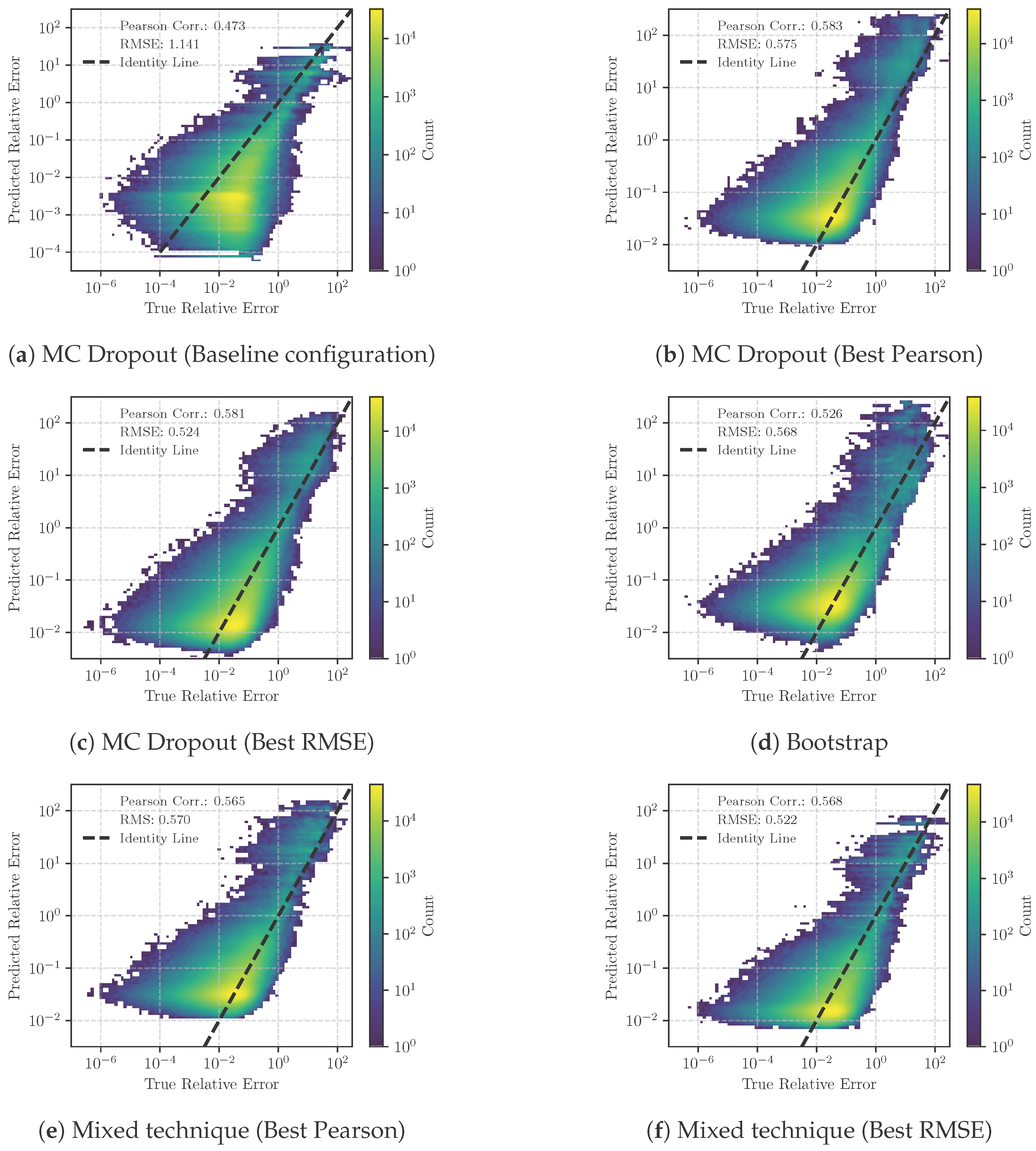
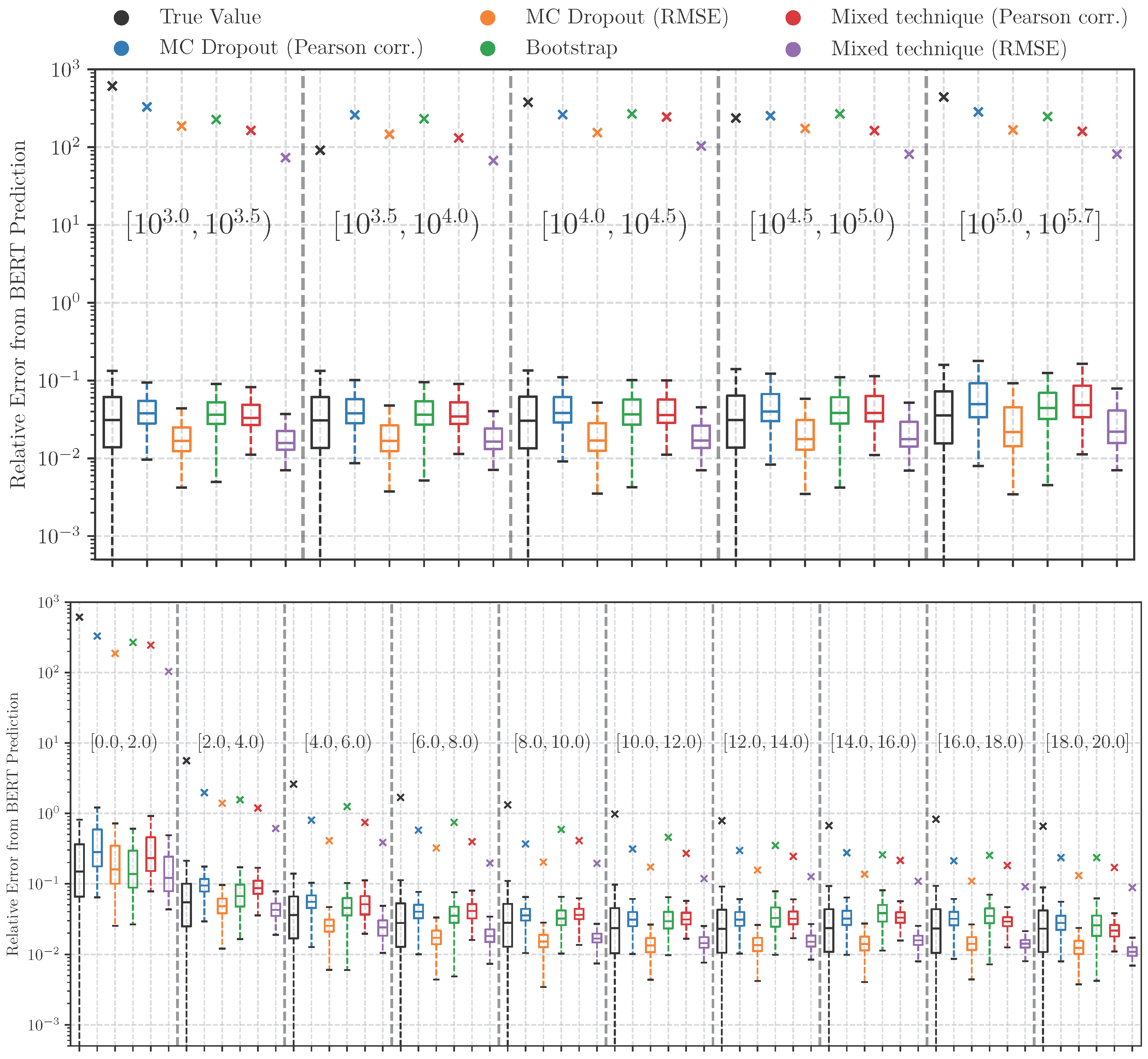
4.2. Results of Uncertainty Estimation

We evaluated various MC dropout configurations for the validation data set, with the results presented in Figure 8, where it is possible to observe how different choices of dropout layers and rates impact the final Pearson correlation and RMSE achieved. By analysing these results, we identified the optimal dropout layer configuration and dropout rate that yield the best performance for both metrics. The best-performing model, marked with a red cross, represents one of the most effective configurations of dropout layers and rates for accurate uncertainty estimation. Although the two selected models share the common characteristic of having dropout activated within the transformer blocks, their dropout rates differ by an order of magnitude and their dropout configuration is not identical. This suggests that, rather than identifying a single optimal configuration, the red crosses may indicate local minima within a broader landscape of nearly equivalent configurations. The observed trend highlights the importance of dropout placement within transformer blocks, but further analysis is needed to determine whether the selected models truly represent the absolute best configurations or if a range of similar setups could achieve comparable performance.

To further inspect the correlation between the Pearson correlation and RMSE, Figure 9 presents the performance of different MC dropout configurations and techniques. Although some configurations show a clear negative correlation, others follow distinct patterns, indicating different behaviours. A smaller subset of configurations achieves overall better error reconstruction, suggesting that a subset of MC dropout settings can be relied upon. Ultimately, the highlighted configurations in Figure 9 represent the best overall choices, although differences within such an optimal cluster of configurations are observed to be minimal.

The selected MC dropout configurations were then used to compose two mixed technique instances, which were also evaluated on the validation data set. The results of this evaluation, along with the bagging method, are presented in Figure 10 in the form of a correlation colour map, showcasing the Pearson correlation and RMSE for each case. It can be seen that the different techniques generally capture the same trends in relative errors, exhibiting similar overall performance. The best Pearson correlation is achieved by the MC dropout model selected based on Pearson correlation, while the best RMSE is obtained by the mixed technique model constructed using the MC dropout configuration with the best RMSE. However, the differences between the various approaches remain relatively minor, suggesting that no single technique provides a significantly superior advantage over the others. In any case, all methods show a clear improvement compared to the baseline configuration, as summarised in

Table 1. Comparison of uncertainty estimation techniques for the relative error in the DA predictions. The Pearson correlation and RMSE is listed, and the best results are highlighted in bold. It should be note that the observed variations are small.

Technique	Validation		Test
	Pearson Correlation	RMSE	Pearson Correlation	RMSE
MC Dropout (Baseline)	0.473	1.141	0.381	0.92
MC Dropout (Best Pearson)	0.583	0.575	0.581	0.575
MC Dropout (Best RMSE)	0.581	0.524	0.579	0.525
Bootstrap Aggregation	0.562	0.568	0.518	0.581
Combined Technique (Best Pearson)	0.565	0.570	0.557	0.574
Combined Technique (Best RMSE)	0.568	0.522	0.560	0.523

.

It should be noted that the true relative error exhibits a wide range of values, ranging from ${10}^{-6}$ to ${10}^2$, while the relative errors predicted by uncertainty estimation techniques are restricted to a narrower range of ${10}^{-2}$ to ${10}^2$. The limited range observed in the predicted uncertainties reflects the inherent constraints of the estimation techniques used. These methods capture the epistemic uncertainty of the model, but they are also influenced by systematic limitations inherent to the techniques used, which cannot be fully eliminated. As a result, the predicted uncertainty cannot fall below a certain threshold even when the model is confident.

In contrast, the actual errors, which we recall are defined as the relative difference between predicted and true values, are not inherently bounded in this way. They can vary freely and, in principle, approach zero when the prediction is highly accurate.

Despite the presence of this lower bound in the predicted uncertainty, its impact on the overall ability of the model to reconstruct the true error remains marginal. The prediction intervals still offer a meaningful characterisation of uncertainty in most of the data range.

To further inspect the resulting relative error distributions achieved by the different techniques, we grouped the relative errors by the number of turns, which corresponds to the input value provided to the network, i.e., the angular DA evaluated at a given number of turns, and by the true angular DA value. The box plots presented in Figure 11 provide an overview of the relative errors obtained for the validation data set, providing the performance of the five selected techniques for the various grouping criteria. The results show that the various methods exhibit a systematic reduced spread in the value of the relative error compared to the true relative errors. This corresponds to the observations made for the correlation plots of Figure 10. However, note that the median values are closed together for all techniques. These characteristics in the reconstructed relative errors highlight the inherent limitations of uncertainty estimation techniques in precisely reproducing the absolute values of the true relative errors. However, in the context of active learning, an exact reconstruction of the error value is not necessarily required. Instead, what matters is the ability to establish a reliable threshold to determine whether a given sample requires further simulation or can be trusted [28]. Given these findings, future active learning strategies should focus on leveraging trends in reconstructed relative errors to guide threshold-based decision making, rather than relying on their absolute values for a perfect reconstruction.

When applied to the test data set, the five selected techniques exhibit performance similar to those observed on the validation data set. The results are consistent across the different grouping criteria, with the models capturing the same trends in the relative errors. The results are summarised in Table 1, which shows how the mixed technique model constructed with the best RMSE MC dropout model is the best-performing technique on the test data set. The MC dropout model selected with the best Pearson correlation also demonstrates a comparable performance, superior to the bagging method. Of course, it is fair to note that the differences between the various techniques are small.

Table 2. Coverage (%) of confidence intervals (CI) for different uncertainty estimation techniques. The technique with the empirical coverage closest to the expected coverage is highlighted in bold. The coverage is computed as the percentage of predictions for which the true DA value falls within the estimated confidence interval.

Technique	68% CI (%)	90% CI (%)	95% CI (%)
MC Dropout (Baseline)	0.3	0.3	0.3
MC Dropout (Best Pearson)	67.1	85.7	90.5
MC Dropout (Best RMSE)	37.1	55.3	62.4
Bootstrap Aggregation	60.8	79.5	84.9
Combined Technique (Best Pearson)	65.3	83.8	88.7
Combined Technique (Best RMSE)	36.7	55.3	62.5

reports the coverage of the predicted confidence intervals for various uncertainty estimation techniques. The baseline MC dropout model, without any tuning, performs poorly, capturing less than 1% of true values in all intervals. In contrast, the configuration optimised for the Pearson correlation achieves the best calibration, with empirical coverages of 67.1%, 85.7%, and 90.5% for the 68%, 90%, and 95% intervals, respectively, values that closely align with expected coverage levels. The bagging and mixed technique also show strong performance, with coverage values approaching expected coverage as well, especially in Pearson-optimised settings. RMSE-optimised techniques perform poorly in terms of calibration, highlighting a trade-off between point prediction accuracy and uncertainty reliability.

When factoring in the computational efficiency of the different approaches, MC dropout emerges as the most effective method for uncertainty estimation. Its ability to provide reliable uncertainty estimates with minimal computational overhead makes it an attractive choice for integrating uncertainty-aware models in accelerator physics applications. The mixed technique, while offering a slight improvement in performance, does not justify the additional computational cost associated with training multiple models. This implies that although the combined method aims at different sources of theoretical uncertainty, it does not produce substantially more information than the techniques applied separately. This observation suggests that the uncertainties addressed by MC dropout and bagging could be derived from similar aspects of the model’s behaviour. Bagging, on the other hand, demonstrates comparable performance to MC dropout but is weak in terms of computational efficiency, limiting its practicality to large-scale systems.

5. Conclusions and Outlook

In this study, we have investigated various techniques for estimating epistemic uncertainty in the prediction of DA using a BERT-based DL model. We evaluated MC dropout, bootstrap aggregation, and a mixed technique that combined both methods to predict uncertainty in DA values. The methods were compared on a large data set of LHC configurations, using the results of the BERT model as a reference for uncertainty estimation. We stress that this study provides a unique opportunity to compare the various techniques to provide epistemic uncertainty against the true uncertainty.

Among the methods evaluated, MC dropout and the mixed technique have shown the best results, although the various methods proved to be rather comparable in providing valid uncertainty estimates. MC dropout also emerges as the most effective technique due to its computational efficiency and ease of integration with existing neural network architectures and the fact that it does not require the retraining of multiple models. This approach not only offers robust uncertainty quantification but also does so with significantly lower computational effort compared to bootstrap aggregation and the explored mixed technique. Furthermore, when optimised for correlation, MC dropout achieves the best coverage in confidence intervals, closely matching the expected coverage.

Our results demonstrate a clear improvement over the MC dropout configurations proposed in previous work. This enhancement is achieved through a series of refinements, including the optimisation of the dropout layer architecture, the introduction of bootstrap aggregation, and the development of a mixed technique combining both approaches. These numerical experiments highlight the importance of carefully selecting the dropout configuration and the uncertainty estimation strategy to improve the quality of uncertainty predictions without incurring significant computational cost. Among the methods tested, our optimised MC dropout approach consistently delivers the best balance between accuracy, robustness, and efficiency. We therefore recommend it as a practical and effective solution for DA uncertainty quantification.

Future efforts will focus on integrating these uncertainty estimation methods into active learning frameworks and further extend these methods to include more beam dynamics effects, such as beam–beam. Using active learning, our aim is to further enhance the efficiency and accuracy of DA predictions, guiding the selection of new data points for simulation based on model uncertainty estimates. This approach promises to optimise computational resources and improve the reliability of surrogate models in accelerator physics applications. Ultimately, the improvement in the uncertainty estimation will enhance the ML framework, leading to more confident decisions on the performance related with accelerator configurations.

References

1. Bazzani, A.; Giovannozzi, M.; Maclean, E.H.; Montanari, C.E.; Van der Veken, F.F.; Van Goethem, W. Advances on the modeling of the time evolution of dynamic aperture of hadron circular accelerators. Phys. Rev. Accel. Beams 2019, 22, 104003. [Google Scholar] [CrossRef]
2. Giovannozzi, M. A proposed scaling law for intensity evolution in hadron storage rings based on dynamic aperture variation with time. Phys. Rev. Spec. Top. Accel. Beams 2012, 15, 024001. [Google Scholar] [CrossRef]
3. Maclean, E.; Giovannozzi, M.; Appleby, R. Innovative method to measure the extent of the stable phase-space region of proton synchrotrons. Phys. Rev. Accel. Beams 2019, 22, 034002. [Google Scholar] [CrossRef]
4. Giovannozzi, M.; Van der Veken, F.F. Description of the luminosity evolution for the CERN LHC including dynamic aperture effects. Part I: The model. Nucl. Instrum. Methods Phys. Res. 2018, A905, 171–179, Erratum in Nucl. Instrum. Methods Phys. Res. 2019, 927, 471. [Google Scholar] [CrossRef]
5. Brüning, O.S.; Collier, P.; Lebrun, P.; Myers, S.; Ostojic, R.; Poole, J.; Proudlock, P. LHC Design Report; CERN Yellow Reports: Monographs; CERN: Geneva, Switzerland, 2004. [Google Scholar] [CrossRef]
6. Apollinari, G.; Béjar Alonso, I.; Brüning, O.; Fessia, P.; Lamont, M.; Rossi, L.; Tavian, L. High-Luminosity Large Hadron Collider (HL–LHC); CERN Yellow Reports: Monographs; CERN: Geneva, Switzerland, 2017; Volume 4. [Google Scholar] [CrossRef]
7. Abada, A.; Abbrescia, M.; AbdusSalam, S.S.; Abdyukhanov, I.; Abelleira Fernandez, J.; Abramov, A.; Aburaia, M.; Acar, A.O.; Adzic, P.R.; Agrawal, P.; et al. FCC-ee: The Lepton Collider. Eur. Phys. J. Spec. Top. 2019, 228, 261–623. [Google Scholar] [CrossRef]
8. Abada, A.; Abbrescia, M.; AbdusSalam, S.S.; Abdyukhanov, I.; Abelleira Fernandez, J.; Abramov, A.; Aburaia, M.; Acar, A.O.; Adzic, P.R.; Agrawal, P.; et al. FCC-hh: The Hadron Collider: Future Circular Collider Conceptual Design Report Volume 3. Eur. Phys. J. Spec. Top. 2019, 228, 755–1107. [Google Scholar] [CrossRef]
9. Skoufaris, K.; Fartoukh, S.; Papaphilippou, Y.; Poyet, A.; Rossi, A.; Sterbini, G.; Kaltchev, D. Numerical optimization of dc wire parameters for mitigation of the long range beam-beam interactions in High Luminosity Large Hadron Collider. Phys. Rev. Accel. Beams 2021, 24, 074001. [Google Scholar] [CrossRef]
10. Droin, C.; Sterbini, G.; Efthymiopoulos, I.; Mounet, N.; De Maria, R.; Tomas, R.; Kostoglou, S.; European Organization for Nuclear Research. Status of beam-beam studies for the high-luminosity LHC. In Proceedings of the IPAC’24—15th International Particle Accelerator Conference, Nashville, TN, USA, 19–24 May 2024; JACoW Publishing: Geneva, Switzerland, 2024; pp. 3213–3216. [Google Scholar] [CrossRef]
11. Assmann, R.W.; Jeanneret, J.B.; Kaltchev, D.I. Efficiency for the imperfect LHC collimation system. In Proceedings of the 8th European Particle Accelerator Conference (EPAC 2002), Paris, France, 3–7 June 2002; p. 293. [Google Scholar]
12. Bracco, C. Commissioning Scenarios and Tests for the LHC Collimation System. Ph.D. Thesis, EPFL, Lausanne, Switzerland, 2008. [Google Scholar]
13. Schenk, M.; Coyle, L.; Pieloni, T.; Giovannozzi, M.; Mereghetti, A.; Krymova, E.; Obozinski, G. Modeling Particle Stability Plots for Accelerator Optimization Using Adaptive Sampling. In Proceedings of the IPAC’21, Campinas, Brazil, 24–28 May 2021; JACoW Publishing: Geneva, Switzerland, 2021; pp. 1923–1926. [Google Scholar] [CrossRef]
14. Casanova, M.; Dalena, B.; Bonaventura, L.; Giovannozzi, M. Ensemble reservoir computing for dynamical systems: Prediction of phase-space stable region for hadron storage rings. Eur. Phys. J. Plus 2023, 138, 559. [Google Scholar] [CrossRef]
15. Devlin, J.; Chang, M.W.; Lee, K.; Toutanova, K. BERT: Pre-training of Deep Bidirectional Transformers for Language Understanding. arXiv 2019, arXiv:1810.04805. [Google Scholar] [CrossRef]
16. Aftan, S.; Shah, H. A Survey on BERT and Its Applications. In Proceedings of the 2023 20th Learning and Technology Conference, Jeddah, Saudi Arabia, 26 January 2023; pp. 161–166. [Google Scholar] [CrossRef]
17. Di Croce, D.; Giovannozzi, M.; Montanari, C.E.; Pieloni, T.; Redaelli, S.; Van der Veken, F.F. Assessing the Performance of Deep Learning Predictions for Dynamic Aperture of a Hadron Circular Particle Accelerator. Instruments 2024, 8, 50. [Google Scholar] [CrossRef]
18. Alizadeh, R.; Allen, J.K.; Mistree, F. Managing computational complexity using surrogate models: A critical review. Res. Eng. Des. 2020, 31, 275–298. [Google Scholar] [CrossRef]
19. Sudret, B.; Marelli, S.; Wiart, J. Surrogate models for uncertainty quantification: An overview. In Proceedings of the 2017 11th European Conference on Antennas and Propagation (EUCAP), Paris, France, 19–24 March 2017; pp. 793–797. [Google Scholar] [CrossRef]
20. Roussel, R.; Edelen, A.L.; Boltz, T.; Kennedy, D.; Zhang, Z.; Ji, F.; Huang, X.; Ratner, D.; Garcia, A.S.; Xu, C.; et al. Bayesian optimization algorithms for accelerator physics. Phys. Rev. Accel. Beams 2024, 27, 084801. [Google Scholar] [CrossRef]
21. Gawlikowski, J.; Tassi, C.R.N.; Ali, M.; Lee, J.; Humt, M.; Feng, J.; Kruspe, A.; Triebel, R.; Jung, P.; Roscher, R.; et al. A survey of uncertainty in deep neural networks. Artif. Intell. Rev. 2023, 56, 1513–1589. [Google Scholar] [CrossRef]
22. Tyralis, H.; Papacharalampous, G. A review of predictive uncertainty estimation with machine learning. Artif. Intell. Rev. 2024, 57, 94. [Google Scholar] [CrossRef]
23. Gal, Y.; Ghahramani, Z. Bayesian Convolutional Neural Networks with Bernoulli Approximate Variational Inference. arXiv 2016, arXiv:1506.02158. [Google Scholar] [CrossRef]
24. Gal, Y.; Hron, J.; Kendall, A. Concrete Dropout. In Proceedings of the Advances in Neural Information Processing Systems, Long Beach, CA, USA, 4–9 December 2017; Guyon, I., Luxburg, U.V., Bengio, S., Wallach, H., Fergus, R., Vishwanathan, S., Garnett, R., Eds.; Curran Associates, Inc.: Red Hook, NY, USA, 2017; Volume 30. [Google Scholar]
25. Gal, Y.; Ghahramani, Z. Dropout as a Bayesian Approximation: Representing Model Uncertainty in Deep Learning. In Proceedings of the 33rd International Conference on International Conference on Machine Learning—ICML’16, New York, NY, USA, 19–24 June 2016; Volume 48, pp. 1050–1059. [Google Scholar]
26. Breiman, L. Bagging predictors. Mach. Learn. 1996, 24, 123–140. [Google Scholar] [CrossRef]
27. Bishop, C.M. Pattern Recognition and Machine Learning, 1st ed.; Information Science and Statistics; Springer: New York, NY, USA, 2006; Volume IV, p. 778. [Google Scholar]
28. Di Croce, D.; Giovannozzi, M.; Krymova, E.; Pieloni, T.; Redaelli, S.; Seidel, M.; Tomás, R.; Van der Veken, F.F. Optimizing dynamic aperture studies with active learning. J. Instrum. 2024, 19, P04004. [Google Scholar] [CrossRef]
29. Kaplan, L.; Cerutti, F.; Sensoy, M.; Preece, A.; Sullivan, P. Uncertainty Aware AI ML: Why and How. arXiv 2018, arXiv:1809.07882. [Google Scholar] [CrossRef]
30. Kabir, H.D.; Mondal, S.K.; Khanam, S.; Khosravi, A.; Rahman, S.; Qazani, M.R.C.; Alizadehsani, R.; Asadi, H.; Mohamed, S.; Nahavandi, S.; et al. Uncertainty aware neural network from similarity and sensitivity. Appl. Soft Comput. 2023, 149, 111027. [Google Scholar] [CrossRef]
31. Tabarisaadi, P.; Khosravi, A.; Nahavandi, S.; Shafie-Khah, M.; Catalão, J.P.S. An Optimized Uncertainty-Aware Training Framework for Neural Networks. IEEE Trans. Neural Netw. Learn. Syst. 2024, 35, 6928–6935. [Google Scholar] [CrossRef]
32. Giovannozzi, M.; Scandale, W.; Todesco, E. Dynamic aperture extrapolation in presence of tune modulation. Phys. Rev. 1998, E57, 3432. [Google Scholar] [CrossRef]
33. Pellegrini, D.; Fartoukh, S.; Karastathis, N.; Papaphilippou, Y. Multiparametric response of the HL-LHC Dynamic Aperture in presence of beam-beam effects. J. Phys. Conf. Ser. 2017, 874, 012007. [Google Scholar] [CrossRef]
34. Jing, Y.C.; Litvinenko, V.; Trbojevic, D. Optimization of Dynamic Aperture for Hadron Lattices in eRHIC. In Proceedings of the 6th International Particle Accelerator Conference (IPAC’15), Richmond, VA, USA, 4 May 2015; p. 757. [Google Scholar] [CrossRef]
35. Cruz Alaniz, E.; Abelleira, J.L.; van Riesen-Hauptpresenter, L.; Seryi, A.; Martin, R.; Tomás, R. Methods to Increase the Dynamic Aperture of the FCC-hh Lattice. In Proceedings of the 9th International Particle Accelerator Conference (IPAC’18), Vancouver, BC, Canada, 3 May 2018; p. 3593. [Google Scholar] [CrossRef]
36. Iadarola, G.; Latina, A.; Abramov, A.; Droin, C.; Demetriadou, D.; Soubelet, F.; Van der Veken, F.; Sterbini, G.; Dilly, J.; Paraschou, K.; et al. Xsuite: An integrated beam physics simulation framework. In Proceedings of the IPAC’24—15th International Particle Accelerator Conference, Nashville, TN, USA, 19–24 May 2024; JACoW Publishing: Geneva, Switzerland, 2024; pp. 2623–2626. [Google Scholar] [CrossRef]
37. Grote, H.; Schmidt, F. MAD-X—An Upgrade from MAD8. In Proceedings of the PAC’03, Portland, OR, USA, 12–16 May 2003; JACoW Publishing: Geneva, Switzerland, 2003; pp. 3497–3499. [Google Scholar] [CrossRef]
38. Deniau, L.; Burkhardt, H.; Maria, R.D.; Giovannozzi, M.; Jowett, J.M.; Latina, A.; Persson, T.; Schmidt, F.; Shreyber, I.S.; Skowroński, P.K.; et al. Upgrade of MAD-X for HL-LHC Project and FCC Studies. In Proceedings of the ICAP’18, Key West, FL, USA, 20–24 October 2018; JACoW Publishing: Geneva, Switzerland, 2018; pp. 165–171. [Google Scholar] [CrossRef]
39. Maria, R.D.; Latina, A.; Schmidt, F.; Dilly, J.; Deniau, L.; Skowronski, P.; Berg, J.; Gläßle, T. Status of MAD-X V5.09. In Proceedings of the IPAC’23—International Particle Accelerator Conference, Venice, Italy, 7–12 May 2023; JACoW Publishing: Geneva, Switzerland, 2023; pp. 3340–3343. [Google Scholar] [CrossRef]
40. MAD—Methodical Accelerator Design. Available online: https://mad.web.cern.ch/mad/ (accessed on 17 July 2025).
41. Hostiadi, D.P.; Atmojo, Y.P.; Huizen, R.R.; Susila, I.M.D.; Pradipta, G.A.; Liandana, I.M. A New Approach Feature Selection for Intrusion Detection System Using Correlation Analysis. In Proceedings of the 2022 4th International Conference on Cybernetics and Intelligent System (ICORIS), Prapat, Indonesia, 8–9 October 2022; pp. 1–6. [Google Scholar] [CrossRef]
42. Parsaei, M.; Taheri, R.; Javidan, R. Perusing The Effect of Discretization of Data on Accuracy of Predicting Naïve Bayes Algorithm. J. Curr. Res. Sci. 2016, 1, 457–462. [Google Scholar]
43. Schmidt, F.; Forest, E.; McIntosh, E. Introduction to the Polymorphic Tracking Code: Fibre Bundles, Polymorphic Taylor Types and “Exact Tracking”; Technical Report CERN-SL-2002-044-AP, KEK-REPORT-2002-3; CERN: Geneva, Switzerland, 2002; Available online: https://cds.cern.ch/record/573082 (accessed on 17 July 2025).
44. Schmidt, F.; Chiu, C.Y.; Goddard, B.; Jacquet, D.; Kain, V.; Lamont, M.; Mertens, V.; Uythoven, J.; Wenninger, J. MAD-X PTC Integration. In Proceedings of the 21st IEEE Particle Accelerator Conference (PAC 2005), Knoxville, TN, USA, 16–20 May 2005; p. 1272. [Google Scholar]
45. Bazzani, A.; Servizi, G.; Todesco, E.; Turchetti, G. A Normal Form Approach to the Theory of Nonlinear Betatronic Motion; CERN Yellow Reports: Monographs; CERN: Geneva, Switzerland, 1994. [Google Scholar] [CrossRef]
46. Abadi, M.; Agarwal, A.; Barham, P.; Brevdo, E.; Chen, Z.; Citro, C.; Corrado, G.S.; Davis, A.; Dean, J.; Devin, M.; et al. TensorFlow: Large-Scale Machine Learning on Heterogeneous Systems. 2015. Available online: https://www.tensorflow.org/ (accessed on 17 July 2025).
47. Pang, B.; Nijkamp, E.; Wu, Y.N. Deep Learning with TensorFlow: A Review. J. Educ. Behav. Stat. 2020, 45, 227–248. [Google Scholar] [CrossRef]
48. Arora, R.; Basu, A.; Mianjy, P.; Mukherjee, A. Understanding Deep Neural Networks with Rectified Linear Units. arXiv 2018, arXiv:1611.01491. [Google Scholar] [CrossRef]
49. Agarap, A.F. Deep Learning using Rectified Linear Units (ReLU). arXiv 2019, arXiv:1803.08375. [Google Scholar] [CrossRef]
50. O’Malley, T.; Bursztein, E.; Long, J.; Chollet, F.; Jin, H.; Invernizzi, L. KerasTuner. 2019. Available online: https://github.com/keras-team/keras-tuner (accessed on 17 July 2025).
51. Vaswani, A.; Shazeer, N.; Parmar, N.; Uszkoreit, J.; Jones, L.; Gomez, A.N.; Kaiser, L.; Polosukhin, I. Attention Is All You Need. arXiv 2023, arXiv:1706.03762. [Google Scholar] [CrossRef]
52. Nguyen, S.; Nguyen, D.; Nguyen, K.; Than, K.; Bui, H.; Ho, N. Structured Dropout Variational Inference for Bayesian Neural Networks. arXiv 2021, arXiv:1909.00719. [Google Scholar] [CrossRef]
53. Foong, A.Y.K.; Burt, D.R.; Li, Y.; Turner, R.E. On the Expressiveness of Approximate Inference in Bayesian Neural Networks. arXiv 2020, arXiv:1909.00719. [Google Scholar] [CrossRef]
54. Joyce, J.M. Kullback-Leibler Divergence. In International Encyclopedia of Statistical Science; Lovric, M., Ed.; Springer: Berlin/Heidelberg, Germany, 2011; pp. 720–722. [Google Scholar] [CrossRef]
55. Murphy, K.P. Machine Learning: A Probabilistic Perspective; MIT Press: Cambridge, MA, USA, 2012. [Google Scholar]
Figure 1. Example of the input data used for evaluating the angular DA, showing the stability radius r s for different angular directions α k and the number of turns N Turns for which the orbit of each initial condition remains bounded. DA prediction performed by our BERT model, presented in the following, is also included. Image adapted from [17].
Computers 14 00287 g001
Figure 2. Sketch of the BERT-based neural network architecture used for DA inference. Image adapted from [17].
Computers 14 00287 g002
Figure 3. Correlation plots of the predicted DA values versus the true DA values obtained from the BERT-based model for the validation (a) and test (b) data sets. The high values of the Pearson correlation coefficients demonstrate the model’s ability to accurately predict DA values across different configurations.
Computers 14 00287 g003
Figure 4. Box plots of the relative errors for the DA prediction from the test data set, considering different grouping criteria. Each box represents the interquartile range (IQR) of the data, with the central line indicating the median, and the whiskers extending to 1.5 times the IQR. Only the top flyer is shown for clarity. (Top) Relative errors grouped by the number of turns, which corresponds to the input value provided to the network, i.e., the angular DA evaluated at a given number of turns. (Bottom) Relative errors grouped by the true DA value. It can be observed that the BERT model tends to exhibit higher relative errors for lower DA values.
Computers 14 00287 g004
Figure 5. Sketch of the trained BERT-based neural network architecture enriched with additional dropout layers for MC dropout.
Computers 14 00287 g005
Figure 6. Convergence of y and σ in the MC dropout estimate for different values of T of an angular DA instance. Top: Impact of the number of samples (shown in the bottom plot) on the uncertainty estimation performance. It can be observed that sufficient stabilisation of y and σ is achieved for T = 128. This specific sampling was performed using configuration 57 with dropout rate 0.001 (details on the dropout configuration are presented in the later sections); comparable trends were observed in the other configurations as well.
Computers 14 00287 g006
Figure 7. Empirical assessment of the Gaussian behaviour of MC dropout samples for two representative configurations. The left plot corresponds to a low-variance case, where the distribution appears nearly deterministic. The right plot shows a higher-variance case, with a distribution that more closely resembles a Gaussian fitted to the sample mean and standard deviation. KL divergence values quantify the deviation from normality in each case, with a value >0.1 indicating significant non-Gaussian behaviour, and a value <0.05 suggesting a good match to Gaussian-like behaviour.
Computers 14 00287 g007
Figure 8. Overview of the achieved performance in predicting the DA uncertainty using different MC dropout configurations and dropout rates. The Pearson correlation (top plot) and mean squared error (central plot) are shown for each configuration, with the best-performing model highlighted with a red cross. The baseline configuration, used in our previous work [28], is highlighted with a red dot. To the side of the colour maps, additional unitary colour maps are included to illustrate the mean values observed when averaging over all configurations that share the same dropout rate or the same dropout layer configuration. These side plots help highlight the effectiveness of specific dropout rates and layer placements. The bottom plot displays the corresponding dropout layer configuration, highlighting which layers were activated during the sampling.
Computers 14 00287 g008
Figure 9. Scatter plot of Pearson correlation versus RMSE for various MC dropout configurations and techniques. The baseline MC dropout configuration, bootstrap aggregation, and the best-performing configurations for each metric (Pearson correlation and RMSE) are highlighted. The results of the combined technique are also included.
Computers 14 00287 g009
Figure 10. Distribution of the correlation between the predicted and true relative error for the BERT model for the validation data set. The Pearson correlation and RMSE are shown for each technique. The results are presented for the MC dropout models selected with the baseline configuration, the best Pearson correlation, and the best RMSE, the bagging method, and the mixed technique models constructed with the best Pearson correlation and the best RMSE MC dropout models. Overall, the performance is the same for all new cases considered, with a significant improvement if compared to the baseline MC dropout configuration.
Computers 14 00287 g010
Figure 11. Box plots of the relative errors for the DA prediction on the validation data set, considering different grouping criteria. Each box represents the interquartile range (IQR) of the data, with the central line indicating the median, and the whiskers extending to 1.5 times the IQR. Only the top flyer is shown for clarity. (Top) Relative errors grouped by the number of turns, which corresponds to the input value provided to the network, i.e., the angular DA evaluated at a given number of turns. (Bottom) Relative errors grouped by the true DA value. It can be observed that all methods capture most of the same trends in the relative errors, demonstrating very similar performance.
Computers 14 00287 g011