An xLSTM–XGBoost Ensemble Model for Forecasting Non-Stationary and Highly Volatile Gasoline Price

Abstract

High-frequency fluctuations in the international crude oil market have led to multilevel characteristics in China’s domestic refined oil pricing mechanism. To address the poor fitting performance of single deep learning models on oil price data, which hampers accurate gasoline price prediction, this paper proposes a gasoline price prediction method based on a combined xLSTM–XGBoost model. Using gasoline price data from June 2000 to November 2024 in Sichuan Province as a sample, the data are decomposed via STL decomposition to extract trend, residual, and seasonal components. The xLSTM model is then employed to predict the trend and seasonal components, while XGBoost predicts the residual component. Finally, the predictions from both models are combined to produce the final forecast. The experimental results demonstrate that the proposed xLSTM–XGBoost model reduces the MAE by 14.8% compared to the second-best sLSTM–XGBoost model and by 83% compared to the traditional LSTM model, significantly enhancing prediction accuracy.

1. Introduction

As an indispensable core energy source in the modern industrial system and residents’ daily lives, gasoline price changes not only affect production costs and consumer expenditures but are also directly related to national energy security and macroeconomic stability [1]. At a time when the global energy structure has not yet been completely transformed, gasoline prices are still a highly sensitive and important variable in economic activities. In recent years, due to the combined effects of multiple factors such as frequent changes in the international political situation, weak global economic recovery, and rapid development of new energy technologies, the international crude oil market has shown high-frequency and large-scale fluctuations [2,3]. This change has a continuous impact on the crude oil pricing mechanism that is transmitted to the entire energy industry chain through the refined oil pricing mechanism, thereby affecting corporate operating costs, government macroeconomic regulation strategies, and residents’ consumption behavior.

China’s refined oil price formation mechanism is based on reference to international oil prices, integrating multidimensional factors such as the tax system, refining costs, and transportation costs, presenting a complex multilevel structure. In this context, price changes are not only reflected in the passive response to international oil prices but are also profoundly affected by regional economic activity and logistics and transportation efficiency. Economically developed regions tend to respond quickly to oil price changes, while remote areas have a certain lag due to insufficient supply chain efficiency. This price spatiotemporal heterogeneity has weakened the optimal allocation efficiency of energy resources to a certain extent, exposing the weak links in the current energy regulation system [4].

At the same time, continuous innovation in energy technology accelerates the reshaping of industrial structures. With the rapid popularization of new energy vehicles, the continuous improvement of the penetration rate of alternative energy such as hydrogen energy and biofuels, as well as the continuous improvement of the efficiency of traditional refining processes, the energy supply and demand relationship has undergone profound changes [5]. As an important signal reflecting the dynamics of the energy market, the prediction accuracy of oil prices has increasingly become a key support for the adjustment of national energy strategies, corporate business decisions, and consumer behavior guidance.

In this context, how to effectively extract the trend, cycle, and disturbance information in the gasoline price series and establish a dynamic prediction model with strong robustness and high generalization ability has become an important topic in the cross-research of energy economics and artificial intelligence [6]. Although the traditional linear time series model has a certain degree of explanatory power, its fitting ability is limited when facing non-stationary and highly volatile oil price data. At the same time, the development of deep learning and machine learning technology has provided new ideas for complex time series modeling [7]. By integrating the advantages of multiple models and combining data decomposition and feature extraction methods, it is possible to more comprehensively characterize the characteristics of oil price fluctuations and improve prediction accuracy and model stability.

Therefore, this study proposes an innovative gasoline price prediction framework by integrating heterogeneous models such as xLSTM and XGBoost, wherein we leverage the sequential learning capability of deep learning and the non-linear fitting strength of ensemble learning. This hybrid approach enhances prediction accuracy and robustness compared to traditional single-model methods. The proposed method not only holds significant theoretical value but also demonstrates broad practical applicability. Its results can serve as a scientific reference for government macro control, corporate procurement strategies, and energy planning. Moreover, it contributes to improving the resilience and flexibility of China’s energy system and promoting the coordinated development of economic efficiency and energy security.

2. Related Work

At present, the literature on gasoline price prediction encompasses a diverse array of methodologies, reflecting the multifaceted nature of the factors influencing fuel prices. Recent research spans traditional statistical models, econometric frameworks, and cutting-edge machine learning approaches, all aimed at enhancing predictive accuracy and offering actionable insights for policy and economic decision making.

A notable contribution is the study by [8], who investigated the relationship between retail gasoline prices and fatal traffic crashes in the United States between 2007 and 2016. Employing random effects negative binomial regression models, the authors revealed that fluctuations in gasoline prices are significantly correlated with traffic safety outcomes, indicating that fuel pricing can have far-reaching societal implications beyond economic metrics. Within the domain of economic theory, Ref. [9] examined the influence of tax policy on gasoline prices, particularly in settings where consumers have imperfect price information. Their findings suggest that the pass-through rate of commodity taxes depends on the proportion of price-sensitive consumers, underscoring the nuanced interplay between regulatory measures and market behavior. Advancements in mathematical modeling are exemplified by [10], who proposed a novel predictive framework for crude oil prices—closely linked to gasoline prices—using a Multivariate Grey Model integrated with a Markov process. This hybrid approach demonstrated superior accuracy compared to conventional models, highlighting the potential of combining grey system theory with probabilistic methods in energy forecasting. The integration of machine learning into gasoline price prediction is further illustrated by [11], who developed a Variational Autoencoder (VAE)-based model to forecast gasoline orders at gas stations in South Korea. By employing clustering and data augmentation techniques to address data asymmetry, the study exemplifies how machine learning can be effectively applied in contexts with limited or imbalanced datasets. The authors in [12] advanced this line of inquiry by applying an Adaptive Network-based Fuzzy Inference System (ANFIS) to predict gasoline prices using comprehensive data from the U.S. Energy Information Administration. Their results emphasize the critical role of historical patterns and temporal dynamics in improving forecast accuracy, with meaningful implications for strategic planning and energy policy development.

In addition, studies by [13,14] focused on the responsiveness of retail gasoline prices to cost shocks. Utilizing large-scale datasets, these works analyzed the pass-through effects of wholesale price fluctuations, revealing a strong correlation between upstream cost changes and retail pricing behavior, thereby enriching the understanding of market transmission mechanisms. Collectively, the existing body of research underscores the value of a multidisciplinary approach that integrates economic theory, statistical analysis, and artificial intelligence. These contributions not only deepen our comprehension of gasoline price dynamics but also provide critical guidance for policymakers, regulators, and industry stakeholders seeking to navigate the complexities of energy markets. However, there are still some key deficiencies: Most methods rely on a single model and find it difficult to cope with the high volatility and non-linear characteristics of oil prices; there is a lack of effective decomposition of time series components such as trends, cycles, and disturbances, which limits feature extraction and modeling capabilities. There is also a lack of regional research, and it is difficult to reflect local economic differences; fusion models often stay at the superposition of result layers and lack a collaborative modeling mechanism based on data characteristics, failing to give full play to the complementary advantages of multiple models.

To address this problem, this paper proposes a user multifeature gasoline price time series data prediction based on the xLSTM–XGBoost combined model. The main contributions are as follows:

• This study first uses the STL (Seasonal and Trend decomposition using Loess) decomposition method to divide the gasoline price time series into trend terms, periodic terms, and residual terms so as to model and predict subsequences with different characteristics separately.
• In the modeling stage, the xLSTM model is used for the period and trend terms to fully explore the long-term dependencies in the time series; the XGBoost model is used to model the residual term, and its powerful non-linear fitting ability is used to make a fine prediction of the residual error. Through this differentiated model selection and collaborative modeling strategy, the accuracy and robustness of the overall prediction are effectively improved.
• The prediction results of the three sub-models are reversely combined according to the STL decomposition logic to obtain the final prediction value of gasoline prices. In the experimental part, the proposed xLSTM–XGBoost combination model is compared with single models (such as LSTM, ARIMA, CNN, and ELM). The results show that the proposed combined model outperforms the existing mainstream methods in terms of prediction accuracy and error control and exhibits stronger adaptability and stability.

3. Hybrid Model Based on ARIMA–xLSTM–XGBoost

This section will focus on introducing the STL decomposition method, xLSTM model, and XGBoost model and give the evaluation indicators MAE, RMSE, $R^2$ for these models.

3.1. STL Decomposition Method

The Seasonal–Trend Decomposition Procedure Based on Loess (STL) is a widely used and highly robust time series analysis technique [15]. Its basic idea is to smooth the time series data through local weighted regression (Loess), thereby effectively decomposing the original series into three independent components: long-term trend, seasonal change, and residual. Compared to traditional time series decomposition techniques such as Classical Decomposition [16], Moving Average Decomposition [17], and Empirical Mode Decomposition (EMD) [18], the STL provides several distinct advantages that make it especially suitable for modeling gasoline prices, which exhibit strong seasonal patterns, non-stationarity, and local volatility. Unlike Classical or Moving Average methods that assume fixed seasonality or are sensitive to noise, the STL is more flexible, allowing seasonality and trends to change over time [19,20]. Moreover, unlike the EMD, which may suffer from mode mixing and which lacks interpretability in financial contexts, The STL’s additive model structure produces interpretable components that align well with economic phenomena—such as long-term pricing trends, periodic tax or supply chain effects, and irregular market shocks. Therefore, the STL was selected in this study, as it offers greater robustness, better decomposition clarity, and adaptability to the high-frequency and volatile characteristics of gasoline price data.

In addition, due to its nature based on locally weighted regression, the STL shows stronger robustness when facing real data containing outliers or non-stationary characteristics [21]. The locally weighted processing mechanism can suppress the influence of extreme values and ensure that the decomposition results will not be disturbed by a small number of abnormal points, thereby providing a more stable and reliable input basis for subsequent modeling and prediction. The schematic diagram of the STL decomposition steps is shown in Figure 1 below. Its mathematical expression is as follows:

$$Y_t=S_t+T_t+R_t$$

(1)

In the equation, $Y_t$ represents the original time series data; $S_t$ represents the seasonal component, that is, the part of the data that changes periodically over time; $T_t$ is the trend component, which reflects the long-term trend of the data over time; and $R_t$ is the residual component, which contains the remaining part after removing seasonality and trend. The overall process of STL decomposition mainly includes the following key steps:

1. Initial Seasonal Estimation Before starting the formal iterative optimization, the STL first makes a preliminary estimate of the seasonal component of the time series. The specific method is to group the time series according to the cycle length of the data (such as 12 for monthly data) and calculate the average value at the same cycle position (such as monthly or quarterly). The initial seasonal estimate obtained in this way provides a good starting point for the subsequent decomposition process and helps to shorten the convergence time of the model.

2. Iterative Refinement The main body of STL decomposition is an iterative optimization process based on the Loess smoother. In each round of iteration, the seasonal term and the trend term are updated alternately to continuously improve the accuracy of the decomposition. Specifically, it includes the following sub-processes:

• Seasonal Extraction: In each round of iteration, the seasonal component is first extracted from the original series by removing the currently estimated trend term and residual term. Then, based on the Loess local regression algorithm, the data points at each periodic position (such as January, February, and December each year) are smoothed to obtain a new seasonal estimate. This process helps capture the periodic laws in the sequence while reducing the interference of trend changes.
• Trend Extraction and Smoothing: After removing the currently updated seasonal term from the sequence, a deseasonalized sequence is obtained. At this point, the Loess smoother is applied again to extract the long-term trend component. This trend estimate can flexibly adapt to nonlinear changes, enabling the model to handle complex trend structures.
• Remainder Calculation: The updated seasonal term and trend term are removed from the original sequence together to obtain the residual part. The residual mainly reflects the short-term random fluctuations or abnormal changes in the data and is a concentrated reflection of the prediction error and unexplainable factors. This step is particularly critical for subsequent outlier detection and model optimization.

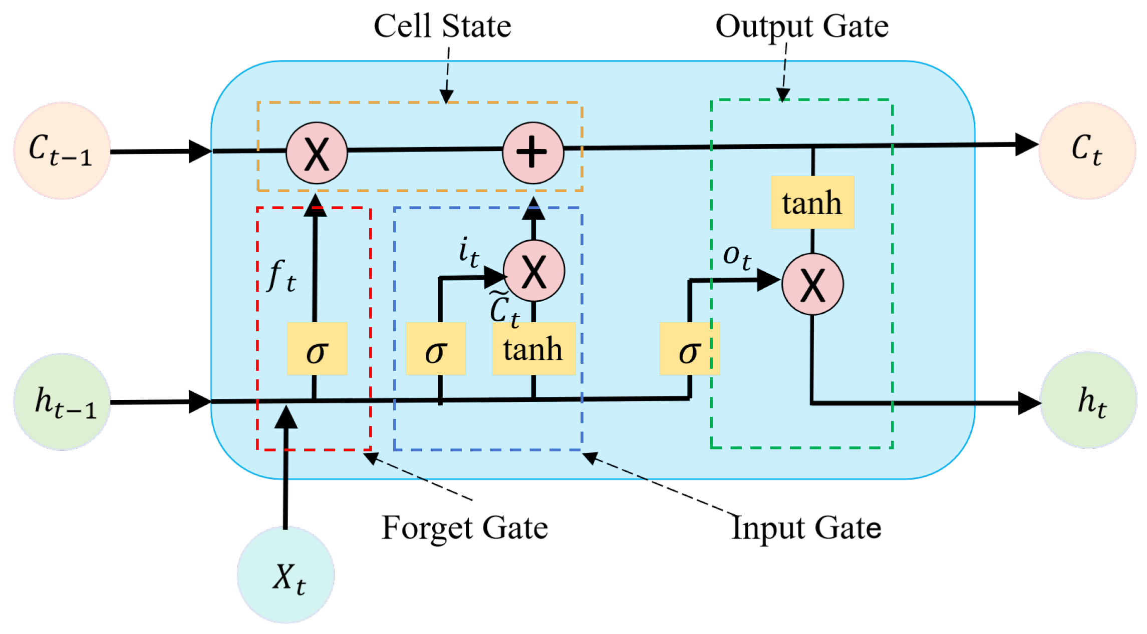
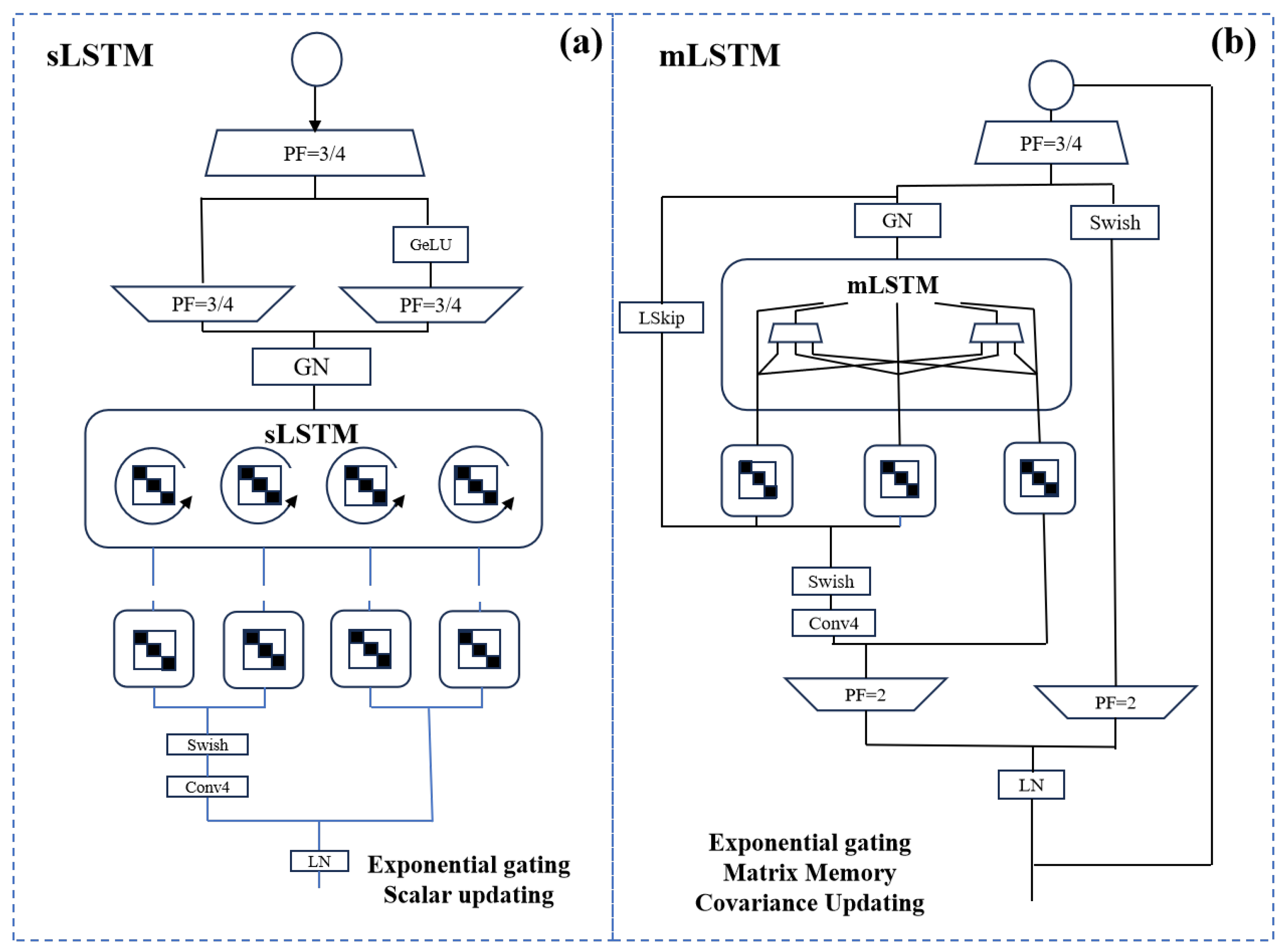
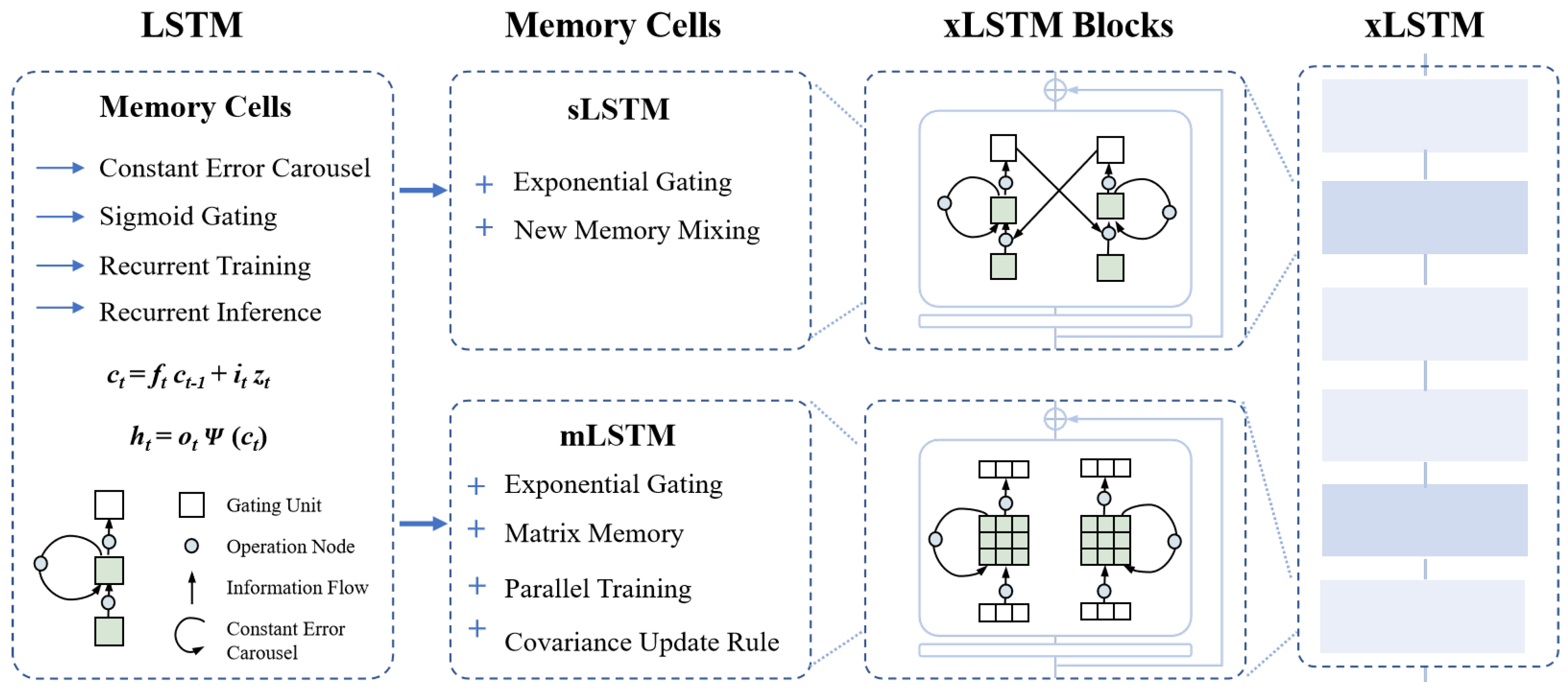
3. Robust Weighting (Optional) In the case of abnormal data points, the STL method provides a robust version. By calculating the median absolute deviation (MAD) of the residual, we can determine whether each data point is an outlier. For points with large deviations, we assign lower weights to reduce their influence in the estimation process of seasonal and trend terms, thereby improving the robustness and stability of the decomposition. This mechanism enables the STL to have strong anti-interference ability and is suitable for actual data environments with large noise.

4. Result synthesis and output As the iteration proceeds, the seasonal and trend estimates gradually stabilize and finally form three parts: long-term trend, cyclical fluctuation components, and random disturbance terms. The sum of the three constitutes a complete reconstruction of the original sequence. This result can not only be used for sequence visualization and analysis but also provides a strong data foundation for subsequent predictive modeling.

5. Boundary processing strategy Since Loess is a local smoothing method based on a sliding window, it is easy to have insufficient data at both ends of the time series (starting and ending positions), which affects the decomposition quality. To solve this boundary effect, techniques such as mirror extension, trend continuation, or endpoint weighting are usually used to fill in the missing data windows at the boundaries, thereby ensuring the stability and continuity of the decomposition results at both ends of the sequence, which reflect the long-term trend of the data over time; therein, r is the residual component, which contains the remaining part after removing seasonality and trend.

3.2. xLSTM Model

LSTM (Long Short-Term Memory) is a specialized type of recurrent neural network (RNN) designed to process and predict time series or sequential data with long-term dependencies [22]. It effectively mitigates the vanishing and exploding gradient problems present in traditional RNNs. The fundamental unit of an LSTM consists of three gating mechanisms—the forget gate, input gate, and output gate—along with a cell state [23,24]. These three gates regulate the flow of information using the sigmoid activation function and element-wise multiplication, ensuring that the strength of the information flow is controlled without introducing additional information. The architecture of an LSTM network is illustrated in Figure 2.

In the Figure 2, $C_{t-1}$ represents the cell state (memory state) at a given time, $X_t$ is the current input, and $h_{t-1}$ denotes the output of the neural unit at time $t-1$. The forget gate’s output at time t is $f_t$, the input gate’s output is $i_t$, and the output gate’s output is $o_t$. The function $\sigma$ represents the sigmoid activation, while $C_t$ is the cell state at time t, and $h_t$ is the neural unit’s output at time t.

To prevent excessive memory retention from interfering with the processing of new inputs, the network selectively forgets certain components of previous cell states while retaining information useful for the current step. The forget gate determines how much of the past information should be preserved in the cell state from time $t-1$. It computes a weight based on $x_t$ and $h_{t-1}$, processes it through a sigmoid activation function, and produces a vector with values between 0 and 1—where 0 signifies information to be forgotten, and 1 denotes information to be retained. The forget gate is mathematically expressed as follows:

$$f_t=\sigma \left(W_f·[h_{t-1},X_t]+b_f\right)$$

(2)

In Equation (2), $W_f$ represents the forget gate weight, $b_f$ denotes the bias, and $\sigma$ is the sigmoid function. The input gate determines how much of the current input information should be retained in the state of the neural unit at the current time step, thereby controlling the information that needs to be updated [25]. The input $X_t$ and $h_{t-1}$ output values pass through the input gate and are then combined with the input and output values processed by a tanh function to generate new control parameters. The mathematical expression for the input gate is as follows:

$$i_t=\sigma (W_i·[h_{t-1},X_t]+b_i)$$

(3)

$${\tilde{C}}_t=tanh(W_c·[h_{t-1},X_t]+b_c)$$

(4)

$$C_t=f_t\ast C_{t-1}+i_t\ast {\tilde{C}}_t$$

(5)

In Equation (5), the cell state is updated as $C_t$, and $W_i$ represents the input gate weight. The output gate determines which information from the current cell state is transmitted to $h_t$. Both $X_t$ and $h_{t-1}$ first pass through the output gate to define the scope of the output information. Then, in combination with the tanh function, a selected $C_t$ portion of the memory information is processed, and the final neural network output value $h_t$ is determined. The mathematical expression for the output gate is as follows:

$$o_t=\sigma (W_o·[h_{t-1},X_t]+b_o)$$

(6)

$$h_t=o_t\ast tanh\left(C_t\right)$$

(7)

In Equations (6) and (7), $W_o$ represents the output gate weight.

The Structural Long Short-Term Memory (sLSTM) network represents a significant advancement over the conventional LSTM model by introducing several architectural and functional enhancements aimed at improving the stability, flexibility, and learning capacity of sequential models [26]. Specifically, sLSTM incorporates exponential gating mechanisms, along with normalization and standardization operations, which together contribute to a more robust and efficient training process. The adoption of an exponential activation function provides finer-grained control over memory retention and forgetting, allowing the network to dynamically adjust the flow of information based on input context. Moreover, to address the instability often encountered during numerical computations in training, sLSTM employs a standardization strategy that accumulates the element-wise product of the input gate and the subsequent forget gates. This approach helps to stabilize gradient propagation and improve convergence behavior. Beyond these improvements, sLSTM is also designed to support multiple memory units within a single time step and introduces a memory mixing mechanism via recurrent links, enabling the model to better capture complex dependencies and interactions across different memory paths. Figure 3a shows the variant sLSTM structure [27]. The sLSTM architecture is divided into three levels from top to bottom: the top layer consists of multiple PF-3/4 modules, which may be used for feature extraction or input preprocessing; the middle layer is composed of GN (gated network) to coordinate multiple sLSTM units with recurrent connections to achieve deep integration of sequence information; the bottom layer includes basic modules such as Switch, Conv4, and LN (layer normalization), combined with Exponential Gating and Scalar Updating mechanisms, to further enhance the dynamic control and state update capabilities of input data. sLSTM emphasizes clear structure and controllable information flow, and is suitable for low- to medium-complexity sequence modeling tasks [28].

In contrast, the Matrix LSTM (mLSTM) extends the representational capacity of LSTM by altering the structure of its memory unit—from a scalar to a matrix form—thereby significantly enhancing its ability to encode and store richer information representations [29,30,31]. This structural change allows the model to concurrently manage multiple key–value memory pairs, making it particularly suitable for tasks requiring complex relational modeling or fine-grained feature retention. Additionally, mLSTM addresses a fundamental limitation of standard LSTMs: their inherent sequential dependency across time steps, which limits parallel computation and increases training time. By removing direct hidden state connections between consecutive time steps, mLSTM enables parallel processing, thus improving computational efficiency [32]. To effectively update and manage the expanded memory structure, mLSTM introduces a covariance-inspired update rule, which facilitates the learning of nuanced patterns and improves the retrieval accuracy of infrequent or rare information instances. Figure 3b shows the variant mLSTM structure. The mLSTM architecture is more complex. In addition to PF-3/4, GN, and Switch modules, its core consists of multiple mLSTM units and introduces the LSkip (cross-layer skip connection) structure to enhance the information flow between different levels, thereby alleviating the gradient problem in deep network training. In addition to common modules, the bottom layer also includes the PF-2 module and integrates the Matrix Memory and Covariance Updating mechanisms, enabling the model to capture more complex correlations between input features. Through Exponential Gating and multidimensional memory structures, mLSTM is more suitable for processing sequence data tasks with complex structures and strong dynamic changes.

xLSTM is a systematic extension and optimization of the traditional LSTM architecture. Its structure integrates a variety of advanced mechanisms to handle complex sequence tasks more efficiently. Its basic module still uses the classic LSTM structure. The core is to introduce memory cells, among which the constant error carousel ensures the continuous propagation of information in time, effectively alleviates the gradient vanishing problem, and enables the model to have the ability to model long-term dependencies. At the same time, the Sigmoid gating mechanism includes an input gate, a forget gate and an output gate, whereby it controls the retention, discarding, and output of information, thereby accurately adjusting state updates. In the training and inference process, the recurrent mechanism [33,34] enables the model to dynamically update its internal state according to the historical context, thereby achieving a gradual understanding of the sequence data.

On this basis, xLSTM introduces two types of improved modules, sLSTM and mLSTM, which are optimized for information flow and memory structure, respectively. sLSTM introduces exponential gating, which provides more detailed information control capabilities than traditional Sigmoid functions, allowing the model to dynamically adjust the gating strength according to different inputs. In addition, the new memory mixing mechanism builds a more efficient fusion channel between new and old information, allowing the model to absorb and utilize new inputs more agilely while retaining historical memory and improving the model’s ability to learn complex and nonlinear data patterns.

Complementary to this, mLSTM strengthens the model’s memory structure and training efficiency. It not only uses exponential gating but also further introduces matrix memory, expanding the memory unit from scalar to matrix form and greatly enhancing the model’s ability to express and manage high-dimensional information, especially for high-dimensional data scenarios such as images and multivariate time series [35]. In order to meet the needs of large-scale data training, mLSTM is also designed with a parallel training mechanism, breaking the traditional serial structure, so that the model training process can more efficiently utilize parallel computing resources (such as GPUs), significantly shortening the training time. At the same time, its Covariance Update Rule optimizes the synergistic relationship between parameters by analyzing the statistical characteristics of the input data, speeding up the model convergence and improving the training stability. These improved modules were unified into xLSTM Blocks with a topological structure. Through the synergy between modules, such as the flexible alternation of gating mechanisms and the complementary fusion of memory management strategies, the entire model has stronger feature expression capabilities and task adaptability. The xLSTM architecture diagram is shown in Figure 4 below.

Table 1. Comparison of LSTM variants.

Model	Full Name	Key Improvements	Suitable Scenarios	Advantages
LSTM	Long Short-Term Memory	Gating mechanism to suppress gradient vanishing	Sequence modeling, language models, time series	Stable and widely used
xLSTM	Extended LSTM	Additional context connections, deeper architecture	Long-range dependencies, complex contexts	Enhanced ability to model long-term dependencies
mLSTM	Multiplicative LSTM	Multiplicative interaction between input and hidden state	Language modeling, NLP	Stronger expressiveness and flexible information control
sLSTM	Structural/Spatial LSTM	Modeling structural or spatial dependencies (e.g., graphs)	GNNs, image and video analysis	Capable of handling dependencies in non-sequential data

compares the key features of the different LSTM variants (LSTM, xLSTM, mLSTM, and sLSTM). The traditional LSTM effectively alleviates the gradient vanishing problem through the gating mechanism and is suitable for general time series modeling. On this basis, xLSTM introduces additional contextual connections and deeper hierarchical structures, enhancing the modeling capabilities of long-term dependencies and complex contexts [36,37]. mLSTM improves the expressiveness of the model by introducing multiplicative interactions between input and hidden states and is suitable for scenarios such as natural language processing. sLSTM is designed for non-sequential data such as graph structures and can model structural or spatial dependencies. This comparison highlights the advantages of xLSTM in processing complex time series data and capturing deep features, which just fits the modeling needs of this article for the long-term dependency and high volatility of gasoline price series.

3.3. XGBoost Model

XGBoost [38] is an efficient and scalable gradient boosting framework. Its core idea is to build decision trees incrementally using an additive model, minimizing prediction errors by optimizing the objective function while also constraining model complexity to improve generalization ability and stability [39]. In each iteration, XGBoost uses a second-order Taylor expansion to approximate the loss function, thereby capturing the variation in the objective function more accurately and accelerating the convergence rate [40]. The objective function of XGBoost combines training error and a regularization term, and its expression is given by

$$Obj=\sum _{i=1}^{n}l(y_i,{\widehat{y}}^{\left(t\right)})+\sum _{k=1}^t\Omega {\left(f_k\right)}^{\iota }$$

(8)

$$\Omega \left(f_k\right)=\gamma T+{\displaystyle \frac{1}{2}}{\lambda \left|\right|\mathbf{\omega }\left|\right|}^2$$

(9)

where $l(y_i,{\widehat{y}}^{\left(t\right)})$ represents the loss value for the i-$th$ sample, and ${\widehat{y}}^{\left(t\right)}$ is the prediction result of the model after the t-th iteration. The regularization term $\Omega \left(f_k\right)$ is used to penalize model complexity, and $\gamma$ and $\lambda$ are the tuning parameters for the number of leaf nodes and the weights of the leaf nodes, respectively.

In each iteration, the model updates the overall output by adding the prediction contribution of the new tree, and its mathematical expression is

$${\widehat{y}}^{\left(t\right)}={\widehat{y}}^{(t-1)}+f_t\left(x_i\right)$$

(10)

where $f_t\left(x_i\right)$ represents the prediction contribution of the t-th tree for the sample $x_i$. This formula reflects the detailed process of how XGBoost approximates the model by progressively accumulating the outputs of decision trees.

3.4. xLSTM–XGBoost Combined Model Prediction Process

The training dataset of this model consisted of the gasoline price data from June 2000 to November 2024 in Sichuan Province, China, with a total of 256 data points. Before predicting gasoline prices, the STL decomposition method was used to decompose the dataset into trend values, residuals, and period values. The STL decomposition method used an additive model and defined a period length of 10. The original sequence was first smoothed using the moving average method to eliminate seasonal fluctuations and noise, capture long-term trends, and obtain trend values. Then, in the sequence after detrending, the mean was calculated by segment according to the period (10 time points) to generate a fixed and repeated seasonal pattern to obtain the period value. Finally, the trend value and period value were subtracted from the original data in turn, and the remaining part was used as the residual to represent unexplained random fluctuations. After STL decomposed the original data, the xLSTM model with adjusted hidden layers was used to predict the trend value and period value, and then the XGBoost model was used to predict the residual data. Finally, the results of the xLSTM and XGBoost predictions were combined using the additive model to obtain the final prediction result. The prediction process of the xLSTM–XGBoost hybrid model is shown in Figure 5 below.

3.5. Evaluation Metrics

This paper usef three representative evaluation metrics to assess the prediction accuracy: the Root Mean Square Error (RMSE), the Mean Absolute Error (MAE), and the Coefficient of Determination ($R^2$). The mathematical expressions for these evaluation metrics are as follows:

$$\mathrm{RMSE}=\sqrt{{\displaystyle \frac{1}{n}}\sum _{i=1}^n{(F_i-R_i)}^2}$$

(11)

$$\mathrm{MAE}=\sum _{i=1}^n{\displaystyle \frac{|F_i-R_i|}{R_i}}$$

(12)

$$R^2=1-{\displaystyle \frac{{\sum }_{i=1}^n{(F_i-A_i)}^2}{{\sum }_{i=1}^n{(F_i-R_i)}^2}}$$

(13)

where $F_i$ is the predicted value for the i-th data point, $R_i$ is the actual value for the i-th data point, n is the sequence length (number of samples), and $A_i$ is the mean of all samples. Smaller values of the RMSE and MAE indicate smaller prediction errors and higher accuracy. $R^2$ takes values between 0 and 1, with a value closer to 1 indicating better fit of the neural network to the data, thus reflecting better model fitting ability.

4. Experimental Design and Results Analysis

The development tool selected for this paper was PyCharm, with the programming language Python 3.11.0. The Graphics Processing Unit (GPU) used was an NVIDIA GeForce GTX 4060, and the Central Processing Unit (CPU) was the i7-13600H, with 6 GB of video memory. The experiment was based on a simulation-generated dataset for prediction, where the dataset was divided into 80% training data and 20% testing data for offset prediction.

4.1. STL Decomposition of Original Data

The dataset used in this study features real-world observational data from the Sichuan Province Data Open Platform, covering monthly gasoline price data from June 2000 to November 2024, with a total of 256 data points. The platform is led by the local government and continuously updated, with high authority and reliability. To ensure data quality, we performed outlier detection and missing value processing after collection to ensure the integrity and consistency of the input data. Due to the representative economic structure and geographical location of Sichuan Province, the selected data offer a certain reference value in capturing regional market volatility and policy transmission mechanisms. In the process of feature processing, the trend value, cycle value, and residual were obtained by decomposing the data using the STL additive model. Figure 6 shows the original data graph of the STL decomposition. This part selects half of the dataset for visualization, including the original data graph, the trend data graph after STL decomposition, the cycle data graph, and the residual graph from top to bottom.

4.2. xLSTM Modeling of Trend and Seasonal Values

The experiment was conducted using a univariate time series dataset (Gasoline Price Trends Dataset), where the data were normalized with MinMaxScaler and split into 80% training and 20% testing sets. Each input sequence consisted of 9 consecutive time steps. Four models were compared: the standard PyTorch LSTM, the parameter-sharing sLSTM, the multihead mLSTM, and the hybrid xLSTM with a combined structure (“msm”). All models took a single input feature (input size = 1) and utilized 64 hidden units. For the multihead variants, two attention heads were employed. The training process ran for 200 epochs with a batch size of 64, using Root Mean Square Error (RMSE) as the loss function and the Adam optimizer for weight updates. Adam was chosen due to its proven ability to adaptively adjust learning rates for individual parameters using moment estimates, which enhances convergence speed and training stability in complex deep learning models. This is particularly important in time series tasks involving volatile and non-stationary data, such as gasoline price prediction. Furthermore, Adam effectively balances bias correction and variance reduction in gradient updates, making it a suitable choice for preventing the optimizer-induced bias that may otherwise distort the learning dynamics in hybrid models like xLSTM [41]. Performance was evaluated based on Mean Absolute Error (MAE), Root Mean Square Error (RMSE), and the Coefficient of Determination ($R^2$). After training, for the data using the LSTM model, the relationship between the true trend value and the predicted trend value was obtained, as shown in Figure 7. In the figure, the blue line represents the original data, and the yellow line represents the result of the trend value prediction. It can be shown from the figure that the model fit is still relatively good.

As can be seen in Figure 7, the LSTM variant model yielded a better prediction effect than the LSTM model, and from the model evaluation indicators in

Table 2. Comparison of LSTM variants in combining trend and seasonal values.

Models	MAE	RMSE	${\mathit{R}}^2$
LSTM	0.3443	0.4137	0.9168
xLSTM	0.0914	0.1118	0.9948
sLSTM	0.1092	0.1321	0.9929
mLSTM	0.1222	0.1468	0.9911

, it can be seen that the prediction effect error of the xLSTM model is lower, and the predicted value is more in line with the true value.

4.3. XGBoost Modeling of Residual Values

Using XGBoost to model the residuals of time series forecasts offers significant advantages. While primary models such as LSTM or ARIMA capture the main trend and seasonality, they may overlook subtle non-linear patterns or irregularities. XGBoost, as a powerful ensemble learner, can effectively learn from these residual errors by modeling their structure, leading to enhanced prediction accuracy. Additionally, XGBoost’s robustness to outliers, built-in regularization, and handling of complex feature interactions make it an excellent choice for residual correction in hybrid forecasting frameworks. This approach improves not only the precision but also the interpretability and stability of the overall time series prediction.

The XGBoost regression model used in this article set 500 trees (n-estimators = 500), a learning rate of 0.1 (learning—rate = 0.1) and a maximum depth of 3 (max-depth = 3), which was done to prevent overfitting while ensuring generalization ability, making it suitable for extracting non-linear features in time series residuals; at the same time, random-state = 42 was set to ensure that the results would be reproducible. The overall model structure is lightweight and suitable for processing stable or less noisy time series data. The following Figure 8 shows the comparison between the prediction results of the XGBoost model for the residual data and the actual values.

4.4. Analysis of Combined Model Prediction Results

The xLSTM–XGBoost combination model proposed in this paper adopts the STL decomposition addition strategy for decomposition. Therefore, the trend and seasonal values predicted by xLSTM and the residual values predicted by XGBoost were added and combined according to the time series to reconstruct the final predicted values. The comparison between the predicted value and the true value of the combination model is shown in Figure 9.

As can be shown from Figure 9, the xLSTM–XGBoost, mLSTM–XGBoost, and sLSTM–XGBoost models based on LSTM variants outperformed the traditional LSTM–XGBoost model in gasoline price prediction. Their predicted values are more closely aligned with the actual values, demonstrating better prediction accuracy and stability. This improvement is attributed to the architectural enhancements in the variant LSTM models: xLSTM introduces extended memory gating and hierarchical structures, mLSTM incorporates matrix-based memory representations for better feature encoding, and sLSTM adopts exponential gating and structural control mechanisms. These modifications significantly enhance the models’ abilities to capture long-term dependencies, handle non-linear patterns, and adapt to local fluctuations in volatile time series.

Furthermore, an examination of the prediction results reveals that the largest errors across all models tended to occur during historically volatile periods, such as the global financial crisis (2008–2009), when oil prices experienced abrupt changes. During these intervals, simpler models like LSTM–XGBoost and ARIMA struggled to adapt to the sudden structural shifts in the data, resulting in higher deviation from the ground truth. In contrast, xLSTM–XGBoost showed a significantly smaller prediction gap in these challenging periods, indicating its superior adaptability to non-stationary patterns and extreme volatility.

Compared to other models shown in

Table 3. Comparison of evaluation indicators for various combination models based on Sichuan Province dataset.

Models	MAE	RMSE	${\mathit{R}}^2$	Training Time (s)
LSTM	0.5644	0.6175	0.8041	35.2
xLSTM	0.3114	0.3906	0.9216	48.6
sLSTM	0.2506	0.3192	0.9476	45.9
mLSTM	0.2619	0.3293	0.9442	49.7
ARIMA	0.6396	0.7203	0.7283	6.3
CNN	0.4178	0.5231	0.1486	38.4
ELM	0.3130	0.4257	0.9154	12.5
LSTM–XGBoost	0.1949	0.2298	0.9782	59.8
sLSTM–XGBoost	0.1129	0.1389	0.9920	57.3
mLSTM–XGBoost	0.1279	0.1547	0.9901	61.2
xLSTM–XGBoost	0.0961	0.1184	0.9942	63.9

, the xLSTM–XGBoost model achieved the lowest MAE and RMSE, with values of 0.0961 and 0.1184, respectively, and the highest R² of 0.9942. These metrics reflect not only improved accuracy but also enhanced model fit and robustness. Specifically, the xLSTM–XGBoost model reduced the MAE by 14.8% compared to the second-best sLSTM–XGBoost and by 83% compared to the standard LSTM model, thereby validating the effectiveness of the proposed hybrid framework in modeling complex and highly volatile gasoline price series.

In order to verify the superiority of the xLSTM–XGBoost combination model over the sLSTM, mLSTM, LSTM, ARIMA, CNN, and ELM models in predicting gasoline price time series data, the prediction results of the seven models were tested by the MAE, RMSE, and $R^2$ evaluation indicators. The results are shown in Table 3. It can be seen from the Table 3 that the evaluation indicators of the xLSTM–XGBoost combination model are superior to those of other single models in all aspects and have a good prediction accuracy. The results of a series of experiments show that the proposed xLSTM–XGBoost model reduced the MAE by 14.8% compared to the sLSTM–XGBoost model and reduced the MAE by 83% compared to the traditional LSTM model. In order to verify the superiority of the xLSTM–XGBoost combination model over the sLSTM, mLSTM, LSTM, ARIMA, CNN, and ELM models in predicting gasoline price time series data, we not only compared the prediction results using the MAE, RMSE, and R² but also conducted statistical significance testing on the performance differences. Specifically, we performed paired sample t-tests and Wilcoxon signed-rank tests on the prediction errors (MAE and RMSE) between the proposed xLSTM–XGBoost model and other baselines on the test set. As shown in

Table 4. Statistical significance testing (xLSTM–XGBoost vs. Others)—t-test p-values for MAE and RMSE.

Model	t-Test p (MAE)	t-Test p (RMSE)
LSTM	$1.08\times {10}^{-14}$	$3.81\times {10}^{-15}$
xLSTM	$3.50\times {10}^{-10}$	$3.61\times {10}^{-11}$
sLSTM	$2.04\times {10}^{-8}$	$1.39\times {10}^{-11}$
mLSTM	$2.91\times {10}^{-8}$	$5.98\times {10}^{-10}$
ARIMA	$1.23\times {10}^{-15}$	$9.43\times {10}^{-16}$
CNN	$9.83\times {10}^{-12}$	$1.78\times {10}^{-12}$
ELM	$5.45\times {10}^{-9}$	$4.75\times {10}^{-12}$
LSTM–xgboost	$1.15\times {10}^{-6}$	$3.30\times {10}^{-8}$
sLSTM–xgboost	$8.53\times {10}^{-2}$	$9.17\times {10}^{-3}$
mLSTM–xgboost	$3.41\times {10}^{-2}$	$1.51\times {10}^{-3}$

, the performance improvements of xLSTM–XGBoost over other models were (p < 0.05) for both MAE and RMSE, indicating that the observed improvements are unlikely due to random chance. This provides strong statistical support for the conclusion that the proposed model demonstrates significantly better performance than the comparative methods.

4.5. Model Generalization Analysis

In order to verify the generalization of the proposed xLSTM–XGBoost model in a limited range, we selected the gasoline price dataset from 2000 to 2024 in Inner Mongolia to verify the generalization of the model and used xLSTM–XGBoost to compare the LSTM–XGBoost, sLSTM–XGBoost, and mLSTM–XGBoost hybrid models.

As shown in Figure 10 and

Table 5. Comparison of evaluation indicators for various combination models based on the Inner Mongolia dataset.

Models	MAE	RMSE	${\mathit{R}}^2$
LSTM–XGBoost	0.5581	0.5827	0.8258
sLSTM–XGBoost	0.1275	0.1476	0.9889
mLSTM–XGBoost	0.1113	0.1297	0.9913
xLSTM–XGBoost	0.1091	0.1274	0.9917

below, the evaluation results of different combination models on this dataset show that the MAE of the LSTM–XGBoost model came out to 0.5581, the RMSE came out to 0.5827, and the R came out to 0.8258. Compared to the other models, its predicted value deviates greatly from the true value, and the fitting effect is poor. The accuracy results of the sLSTM–XGBoost model and the mLSTM–XGBoost model are further improved by comparison. The xLSTM–XGBoost model performed best, with a MAE of 0.1091, a RMSE of 0.1274, and an R of 0.9917, with the highest prediction accuracy and the best data fitting effect. It can be seen that the xLSTM–XGBoost hybrid model also has relatively good accuracy on other datasets.

5. Conclusions

In order to solve the problem that a single deep learning model has a poor fitting effect on oil price data, which makes it difficult to predict gasoline prices, this paper proposes an xLSTM–XGBoost combined model to predict gasoline prices. First, the gasoline price time series data are decomposed into trend values, period values, and residuals using STL decomposition. Then, the xLSTM model is used to predict the trend values and seasonal values, and XGBoost is used to predict the residual values. Finally, the prediction results of the two models are combined to obtain the final prediction results. The experimental results show that compared to the classic LSTM, ARIMA, CNN, and other single models, the proposed xLSTM–XGBoost combined model has higher prediction accuracy and better fitting results.

However, this study still has several limitations. First, although STL decomposition improves interpretability, it relies on fixed periodicity assumptions and may not adapt well to structural breaks or regime shifts in the time series. Secondly, the model does not yet incorporate external influencing variables (e.g., international crude oil futures, exchange rates, and macroeconomic indicators), which could potentially enhance its prediction accuracy and explanatory power.

Future research will focus on the following directions: (1) exploring adaptive decomposition techniques (e.g., wavelet transform or empirical mode decomposition) to handle non-periodic or evolving patterns and (2) integrating exogenous variables and developing a multivariate version of the hybrid model. Furthermore, introducing uncertainty quantification methods (such as Bayesian inference or quantile regression) will be considered to improve the reliability and decision-making value of the predictions.

References

1. Hasanov, F.J.; Javid, M.; Mikayilov, J.I.; Shabaneh, R.; Darandary, A.; Alyamani, R. Macroeconomic and sectoral effects of natural gas price: Policy insights from a macroeconometric model. Energy Econ. 2025, 143, 108233. [Google Scholar] [CrossRef]
2. Mao, Z.; Suzuki, S.; Nabae, H.; Miyagawa, S.; Suzumori, K.; Maeda, S. Machine learning-enhanced soft robotic system inspired by rectal functions to investigate fecal incontinence. Bio-Des. Manuf. 2025, 8, 482–494. [Google Scholar] [CrossRef]
3. Mao, Z.; Kobayashi, R.; Nabae, H.; Suzumori, K. Multimodal strain sensing system for shape recognition of tensegrity structures by combining traditional regression and deep learning approaches. IEEE Robot. Autom. Lett. 2024, 9, 10050–10056. [Google Scholar] [CrossRef]
4. Khanna, A.A.; Dubernet, I.; Jochem, P. Do car drivers respond differently to fuel price changes? Evidence from German household data. Transportation 2025, 52, 579–613. [Google Scholar] [CrossRef]
5. Kamocsai, L.; Ormos, M. Modeling gasoline price volatility. Financ. Res. Lett. 2025, 73, 106657. [Google Scholar] [CrossRef]
6. Safaei, N.; Zhou, C.; Safaei, B.; Masoud, A. Gasoline prices and their relationship to the number of fatal crashes on US roads. Transp. Eng. 2021, 4, 100053. [Google Scholar] [CrossRef]
7. Mao, Z.; Bai, X.; Peng, Y.; Shen, Y. Design, modeling, and characteristics of ring-shaped robot actuated by functional fluid. J. Intell. Mater. Syst. Struct. 2024, 35, 1459–1470. [Google Scholar] [CrossRef]
8. Montag, F.; Sagimuldina, A.; Schnitzer, M. Does Tax Policy Work When Consumers Have Imperfect Price Information? Theory and Evidence; Technical Report, CESifo Working Paper; The MIT Press: Cambridge, MA, USA, 2021. [Google Scholar]
9. Indrakala, S. A study on mathematical methods for predicting accuracy of crude oil futures prices by multi grey Markov model. Malaya J. Mat. 2021, 9, 621–626. [Google Scholar] [CrossRef]
10. Li, W.; Becker, D.M. Day-ahead electricity price prediction applying hybrid models of LSTM-based deep learning methods and feature selection algorithms under consideration of market coupling. Energy 2021, 237, 121543. [Google Scholar] [CrossRef]
11. Noel, M. Do retail gasoline prices respond asymmetrically to cost shocks? The influence of Edgeworth Cycles. Rand J. Econ. 2009, 40, 582–595. [Google Scholar] [CrossRef]
12. Yoon, S.; Park, M. Prediction of gasoline orders at gas stations in South Korea using VAE-based machine learning model to address data asymmetry. Appl. Sci. 2023, 13, 11124. [Google Scholar] [CrossRef]
13. Eliwa, E.H.I.; El Koshiry, A.M.; Abd El-Hafeez, T.; Omar, A. Optimal gasoline price predictions: Leveraging the ANFIS regression model. Int. J. Intell. Syst. 2024, 2024, 8462056. [Google Scholar] [CrossRef]
14. He, M.; Qian, X. Forecasting tourist arrivals using STL-XGBoost method. Tour. Econ. 2025, 13548166241313411. [Google Scholar] [CrossRef]
15. Cardona, G.A.; Kamale, D.; Vasile, C.I. STL and wSTL control synthesis: A disjunction-centric mixed-integer linear programming approach. Nonlinear Anal. Hybrid Syst. 2025, 56, 101576. [Google Scholar] [CrossRef]
16. Luo, S.; Lambert, N.; Liang, P.; Cirio, M. Quantum-classical decomposition of Gaussian quantum environments: A stochastic pseudomode model. PRX Quantum 2023, 4, 030316. [Google Scholar] [CrossRef]
17. Singh, S.; Parmar, K.S.; Kumar, J.; Makkhan, S.J.S. Development of new hybrid model of discrete wavelet decomposition and autoregressive integrated moving average (ARIMA) models in application to one month forecast the casualties cases of COVID-19. Chaos Solitons Fractals 2020, 135, 109866. [Google Scholar] [CrossRef] [PubMed]
18. Rehman, N.; Mandic, D.P. Multivariate empirical mode decomposition. Proc. R. Soc. A Math. Phys. Eng. Sci. 2010, 466, 1291–1302. [Google Scholar] [CrossRef]
19. Peng, Y.; Yang, X.; Li, D.; Ma, Z.; Liu, Z.; Bai, X.; Mao, Z. Predicting flow status of a flexible rectifier using cognitive computing. Expert Syst. Appl. 2025, 264, 125878. [Google Scholar] [CrossRef]
20. Peng, Y.; Sakai, Y.; Funabora, Y.; Yokoe, K.; Aoyama, T.; Doki, S. Funabot-Sleeve: A Wearable Device Employing McKibben Artificial Muscles for Haptic Sensation in the Forearm. IEEE Robot. Autom. Lett. 2025, 10, 1944–1951. [Google Scholar] [CrossRef]
21. Chen, Y.; Liu, X.; Rao, M.; Qin, Y.; Wang, Z.; Ji, Y. Explicit speed-integrated LSTM network for non-stationary gearbox vibration representation and fault detection under varying speed conditions. Reliab. Eng. Syst. Saf. 2025, 254, 110596. [Google Scholar] [CrossRef]
22. Yuan, F.; Huang, X.; Zheng, L.; Wang, L.; Wang, Y.; Yan, X.; Gu, S.; Peng, Y. The evolution and optimization strategies of a PBFT consensus algorithm for consortium blockchains. Information 2025, 16, 268. [Google Scholar] [CrossRef]
23. Wang, X.; Yu, H.; Kold, S.; Rahbek, O.; Bai, S. Wearable sensors for activity monitoring and motion control: A review. Biomim. Intell. Robot. 2023, 3, 100089. [Google Scholar] [CrossRef]
24. Wen, X.; Wang, Y.; Zhu, Q.; Wu, J.; Xiong, R.; Xie, A. Design of recognition algorithm for multiclass digital display instrument based on convolution neural network. Biomim. Intell. Robot. 2023, 3, 100118. [Google Scholar] [CrossRef]
25. Yu, Y.; Si, X.; Hu, C.; Zhang, J. A review of recurrent neural networks: LSTM cells and network architectures. Neural Comput. 2019, 31, 1235–1270. [Google Scholar] [CrossRef]
26. Mariappan, Y.; Ramasamy, K.; Velusamy, D. An optimized deep learning based hybrid model for prediction of daily average global solar irradiance using CNN SLSTM architecture. Sci. Rep. 2025, 15, 10761. [Google Scholar] [CrossRef]
27. Alharthi, M.; Mahmood, A. xlstmtime: Long-term time series forecasting with xlstm. AI 2024, 5, 1482–1495. [Google Scholar] [CrossRef]
28. Schmied, T.; Adler, T.; Patil, V.; Beck, M.; Pöppel, K.; Brandstetter, J.; Klambauer, G.; Pascanu, R.; Hochreiter, S. A Large Recurrent Action Model: xLSTM enables Fast Inference for Robotics Tasks. arXiv 2024, arXiv:2410.22391. [Google Scholar] [CrossRef]
29. Zhou, Y.; Zhou, S.; Cheng, D.; Li, J.; Hua, Z. STDF: Joint Spatiotemporal Differences Based on xLSTM Dendritic Fusion Network for Remote Sensing Change Detection. IEEE J. Sel. Top. Appl. Earth Obs. Remote Sens. 2025, 18, 1–16. [Google Scholar] [CrossRef]
30. Ni, J.; Chen, Y.; Tang, G.; Shi, J.; Cao, W.; Shi, P. Deep learning-based scene understanding for autonomous robots: A survey. Intell. Robot. 2023, 3, 374–401. [Google Scholar] [CrossRef]
31. Mao, Z.; Suzuki, S.; Wiranata, A.; Zheng, Y.; Miyagawa, S. Bio-inspired circular soft actuators for simulating defecation process of human rectum. J. Artif. Organs 2025, 28, 252–261. [Google Scholar] [CrossRef]
32. Shen, Z.; Jiang, Z.; Zhang, J.; Wu, J.; Zhu, Q. Learning-based robot assembly method for peg insertion tasks on inclined hole using time-series force information. Biomim. Intell. Robot. 2025, 5, 100209. [Google Scholar] [CrossRef]
33. Pöppel, K.; Beck, M.; Spanring, M.; Auer, A.; Prudnikova, O.; Kopp, M.K.; Klambauer, G.; Brandstetter, J.; Hochreiter, S. xlstm: Extended long short-term memory. In Proceedings of the First Workshop on Long-Context Foundation Models@ ICML 2024, Vienna, Austria, 21–27 July 2024. [Google Scholar] [CrossRef]
34. Kühne, N.L.; Østergaard, J.; Jensen, J.; Tan, Z.H. xLSTM-SENet: xLSTM for Single-Channel Speech Enhancement. arXiv 2025, arXiv:2501.06146. [Google Scholar] [CrossRef]
35. Li, Y.; Zhang, H.; Zhang, X.; Feng, H. Multi-scale Attention-based xLSTM for Rolling Bearing Fault diagnosis. Meas. Sci. Technol. 2025, 36, 066116. [Google Scholar] [CrossRef]
36. He, H.; Liao, R.; Li, Y. MSAFNet: A novel approach to facial expression recognition in embodied AI systems. Intell. Robot. 2025, 5, 313–332. [Google Scholar] [CrossRef]
37. Li, J.; Yang, S.X. Digital twins to embodied artificial intelligence: Review and perspective. Intell. Robot. 2025, 5, 202–227. [Google Scholar] [CrossRef]
38. Chen, T.; Guestrin, C. Xgboost: A scalable tree boosting system. In Proceedings of the 22nd ACM Sigkdd International Conference on Knowledge Discovery and Data Mining, San Francisco, CA, USA, 13–17 August 2016; pp. 785–794. [Google Scholar] [CrossRef]
39. Dhaliwal, S.S.; Nahid, A.A.; Abbas, R. Effective intrusion detection system using XGBoost. Information 2018, 9, 149. [Google Scholar] [CrossRef]
40. Li, J.; An, X.; Li, Q.; Wang, C.; Yu, H.; Zhou, X.; Geng, Y.a. Application of XGBoost algorithm in the optimization of pollutant concentration. Atmos. Res. 2022, 276, 106238. [Google Scholar] [CrossRef]
41. Mavrogiorgos, K.; Kiourtis, A.; Mavrogiorgou, A.; Menychtas, A.; Kyriazis, D. Bias in Machine Learning: A Literature Review. Appl. Sci. 2024, 14, 8860. [Google Scholar] [CrossRef]
Figure 1. STL decomposition steps diagram.
Computers 14 00256 g001
Figure 2. LSTM architecture diagram.
Computers 14 00256 g002
Figure 3. Variants of the Long Short-Term Memory (LSTM) architecture. Among them, (a) is the sLSTM model architecture diagram. (b) is the mLSTM model architecture diagram.
Computers 14 00256 g003
Figure 4. xLSTM architecture diagram.
Computers 14 00256 g004
Figure 5. xLSTM–XGBoost combined model prediction flow chart.
Computers 14 00256 g005
Figure 6. STL decomposition of the original data.
Computers 14 00256 g006
Figure 7. Comparison chart of trend and seasonal value predictions by various models.
Computers 14 00256 g007
Figure 8. Comparison of XGBoost model prediction residual values.
Computers 14 00256 g008
Figure 9. Inner Mongolia dataset Comparison of gasoline price forecasts by various combination models based on Sichuan Province dataset.
Computers 14 00256 g009
Figure 10. Comparison of gasoline price forecasts by various combination models based on the Inner Mongolia dataset.
Computers 14 00256 g010