Article

An Efficient Hybrid 3D Computer-Aided Cephalometric Analysis for Lateral Cephalometric and Cone-Beam Computed Tomography (CBCT) Systems

by
Laurine A. Ashame
1,*,
Sherin M. Youssef
1,*,
Mazen Nabil Elagamy
1 and
Sahar M. El-Sheikh
2
1
Computer Engineering Department, College of Engineering and Technology, Arab Academy for Science, Technology and Maritime Transport, Abu Qir, Alexandria 1029, Egypt
2
Department of Oral Pathology, Faculty of Dentistry, Alexandria University, Alexandria 21521, Egypt
*
Authors to whom correspondence should be addressed.
Computers 2025, 14(6), 223; https://doi.org/10.3390/computers14060223 (registering DOI)
Submission received: 4 April 2025 / Revised: 7 May 2025 / Accepted: 12 May 2025 / Published: 7 June 2025
(This article belongs to the Special Issue Machine Learning Applications in Pattern Recognition)

Abstract

:
Lateral cephalometric analysis is commonly used in orthodontics for skeletal classification to ensure an accurate and reliable diagnosis for treatment planning. However, most current research depends on analyzing different type of radiographs, which requires more computational time than 3D analysis. Consequently, this study addresses fully automatic orthodontics tracing based on the usage of artificial intelligence (AI) applied to 2D and 3D images, by designing a cephalometric system that analyzes the significant landmarks and regions of interest (ROI) needed in orthodontics tracing, especially for the mandible and maxilla teeth. In this research, a computerized system is developed to automate the tasks of orthodontics evaluation during 2D and Cone-Beam Computed Tomography (CBCT or 3D) systems measurements. This work was tested on a dataset that contains images of males and females obtained from dental hospitals with patient-informed consent. The dataset consists of 2D lateral cephalometric, panorama and CBCT radiographs. Many scenarios were applied to test the proposed system in landmark prediction and detection. Moreover, this study integrates the Grad-CAM (Gradient-Weighted Class Activation Mapping) technique to generate heat maps, providing transparent visualization of the regions the model focuses on during its decision-making process. By enhancing the interpretability of deep learning predictions, Grad-CAM strengthens clinical confidence in the system’s outputs, ensuring that ROI detection aligns with orthodontic diagnostic standards. This explainability is crucial in medical AI applications, where understanding model behavior is as important as achieving high accuracy. The experimental results achieved an accuracy exceeding 98.9%. This research evaluates and differentiates between the two-dimensional and the three-dimensional tracing analyses applied to measurements based on the practices of the European Board of Orthodontics. The results demonstrate the proposed methodology’s robustness when applied to cephalometric images. Furthermore, the evaluation of 3D analysis usage provides a clear understanding of the significance of integrated deep-learning techniques in orthodontics.

1. Introduction

The global market of AI in healthcare, including dentistry, was valued at USD 20.9 billion in 2024, and is expected to reach USD 148.4 billion by 2029, growing at a compound annual growth rate (CAGR) of 48.1%. This rapid growth demonstrates the transformative potential of AI in healthcare, including dentistry [1]. Recently, much research has been undertaken to understand genetic mechanisms that control the development of dental pathologies. One of the main problems ahead is related to further elucidating how genes contribute to diseases with a complex inheritance pattern. Almost every aspect of oral health is affected to a degree by genes.
Population studies indicate that tooth agenesis can occur either as an isolated trait or as part of a broader syndrome. Isolated cases may arise sporadically or follow a familial pattern, with inheritance linked to dominant, recessive, or X-linked genetic mechanisms [2]. While the genetic basis of third molar agenesis is complex and often cannot be fully explained by a simple autosomal dominant model, research suggests that a polygenic mode of inheritance plays a significant role. Beyond the absence of certain teeth, tooth agenesis can contribute to malocclusion by disrupting occlusal harmony, affecting dental arch integrity, and leading to functional and aesthetic concerns. The absence of key teeth may result in spacing irregularities, altered eruption patterns, and compensatory dental shifts, all of which can influence bite alignment and overall craniofacial development. Grahnen [3] stated that tooth agenesis is typically transmitted as an autosomal dominant trait with incomplete penetrance and variable expressivity. Twin studies have been widely used to show the importance of the genetic component involved during tooth development to control both tooth size and form. There are numerous case reports suggesting concordance for tooth agenesis in monozygotic twins, and case reports where variation in the expressivity is observed.
Lateral cephalometry is a fundamental tool applied in orthodontics and oral health, and is widely utilized for evaluating dental, skeletal, and soft tissue structures [4]. Its role in orthodontic diagnosis is essential, particularly for skeletal classification and treatment planning. By analyzing cephalometric images, clinicians can assess jaw alignment, growth patterns, and facial proportions, guiding treatment decisions for malocclusions and other orthodontic concerns. Traditionally, this process requires the manual identification of key cephalometric landmarks, followed by complex linear and angular measurements. However, while precise landmark identification is crucial for accurate analysis, it is also highly time-consuming and prone to human errors and variability. Advancements in digital automation and AI-assisted cephalometric analysis aim to enhance accuracy and efficiency, reducing the potential for inconsistencies in orthodontic assessments [5]. Cephalometric analysis is essential for evaluating skeletal structures, dental alignment, and overall facial balance. This process relies on key anatomical landmarks to ensure precise measurements. For skeletal assessment, reference points such as Sella (S) and Nasion (N) help define the cranial base, while A Point and B Point provide insight into the positioning of the upper and lower jaws. Additionally, Pogonion (Pg) and Menton (Me) are crucial to analyzing chin prominence and symmetry. Dental landmarks also play a pivotal role in cephalometric analysis. The Upper Incisor and Lower Incisor are examined to assess tooth angulation and alignment, while the First Molar is used to evaluate occlusal relationships and overall bite stability. By integrating these landmarks into cephalometric evaluations, orthodontists can develop accurate diagnoses, predict growth patterns, and design effective treatment strategies. Advancements in digital imaging and AI-driven cephalometric analysis continue to refine precision, improving diagnostic efficiency and minimizing human error in orthodontic assessments.
Applying the AI algorithm to CBCT can offer analyses of images at almost the same level of quality as experienced clinicians, who represent the current gold standard [6]. This study is one of the first to successfully enable the implementation of AI in dentistry, in particular orthodontics, satisfying medical requirements by reducing the number of landmarks used in 2D tracing.
Moreover, various current orthodontic diagnostic methods that have been standardized over time rely on dozens of manually identified landmarks on the lateral cephalogram and panorama radiographs. The two-step “detection–diagnosis” method of landmark analysis is prone to human errors and the loss of useful diagnostic information. Artificial intelligence can be used in various phases of orthodontics, from diagnosis to treatment planning and follow-up monitoring, using 3D images to reach a precise analysis in a desirable time [7].
The early identification of dental and skeletal abnormalities plays a crucial role in orthodontic diagnosis, enhancing prognosis and minimizing the risk of malocclusion. The integration of 3D scans and virtual models allows for the development of sophisticated data algorithms to intelligently assess the precise positioning of teeth, enabling more accurate evaluations. To foster optimal maxillofacial development, a hybrid clinical approach should be implemented at the earliest stages, ensuring balanced and harmonious growth [8].
Additionally, using Grad-CAM in heatmap generation can show which parts of the image are most important to the model, being a tool that shows how a deep learning model makes its decisions. It creates a heatmap that helps in understanding what a deep learning model is thinking. It highlights the key areas of the image that influence the model’s performance. This is extremely useful in improving model transparency, and making the model’s decisions more reliable. Despite the promising results achieved by the proposed AI-based system for orthodontic evaluation, several limitations remain that could impact the performance of AI when applied in teeth detection. First, variabilities in radiograph quality, such as differences in contrast, resolution, and the presence of artifacts, can adversely affect landmark detection and segmentation accuracy. Additionally, anatomical variations among patients, including age-related changes, missing or overlapping teeth, or pathological conditions, introduce complexity that may challenge the generalizability of the trained models. Another limitation lies in the dependency on large, high-quality, and diverse annotated datasets; insufficient or biased data can lead to reduced model performance and overfitting. Moreover, while techniques like Grad-CAM improve interpretability, the decision boundaries of deep learning models still remain partially opaque, potentially raising concerns about reliability in critical clinical decisions. Finally, artificial intelligence (AI) holds promise in greatly simplifying and speeding up genome interpretation by integrating predictive methods with the growing knowledge of genetic dental abnormalities.

1.1. Biological Background

The basic physical and functional unit of heredity is the gene, which is found in DNA. Genetics plays a direct role in influencing dentistry. Several genetic factors can affect dental and skeletal aspects [9]. These factors can determine the alignment, shape, and size of the teeth, as well as the skeletal relations between the maxilla and mandible, regardless of dental habits. This is illustrated in Figure 1. Genetics play a significant role in shaping orthodontic outcomes, influencing everything from jaw structure to how teeth align. Inherited traits can determine factors like tooth size, eruption patterns, and the likelihood of conditions such as crowding or overbites. Certain genetic variations may predispose individuals to skeletal imbalances, making early assessment crucial for effective treatment. With advancements in genetic research, orthodontists can now better understand these hereditary influences, allowing for more personalized care tailored to each patient’s unique biological makeup. By integrating genetic insights into treatment planning, orthodontic interventions can be made more predictive and proactive, and optimized for long-term stability.
Malocclusion, also known as “bad bite”, is a common dental issue. The malocclusion is defined as a lack of alignment between upper and lower teeth. Malocclusion typically happens when teeth are crowded or spaced apart, meaning the teeth are too large for the mouth or the mouth is too large for the teeth [10]. In malocclusion, there are three classes—class 1 is named orthognathic or mesognathic (which are not the same but are related), and is a normal variation based on the standard deviation determined statistically by the European Board of Orthodontics. In a normal molar relationship, the mesiobuccal cusp of the upper first molar fits into the mesiobuccal groove of the lower first molar. For the canines, the front slope of the upper canine meets the back slope of the lower canine, and the back slope of the upper canine touches the front slope of the first lower premolar. The line of occlusion is often altered due to issues like crowding, spacing, or bite problems such as open bite, deep bite, or crossbite. A mesognathic profile refers to a straight, balanced facial appearance. Class 2 is retrognathic (overjet); in this case, the molar relationship is defined by the lower first molar positioned slightly behind the upper first molar, with the upper molar’s cusp resting between the lower first molar and the second premolar. For the canines, the front slope of the upper canine sits ahead of the lower canine, with the lower canine sitting further back by about the width of a premolar. The line of occlusion is irregular and varies depending on facial structure, crowding, or spacing. The retrognathic profile features a convex face due to a small lower jaw or a large upper jaw. Finally, class 3 is prognathic; in this case, the upper first molar’s cusp sits behind the groove of the lower first molar. The lower canines are shifted forward compared to the upper canines by about the width of a premolar, and the lower front teeth are in full crossbite. The line of occlusion is irregular, often influenced by facial shape, crowding, or spacing. A prognathic profile, with a prominent lower jaw, is linked to Class III malocclusion, as shown in Figure 1a. Moreover, Figure 1b shows an example of a 2D lateral cephalometric of malocclusion “bad bite”, and its line tracing.
Skeletal classification is an important part of orthodontic diagnosis and treatment planning, assessed by the vertical and anteroposterior positions of the jaws in lateral cephalograms. The assessment helps clinicians predict various growth patterns such as the direction of condylar growth or dentoalveolar development planning [11]. Thus, accurate diagnosis based on proper landmark identification and analysis has been considered essential to successful usage.

1.1.1. Characteristic of CBCT

CBCTs are 3D X-rays and a variation of traditional computed tomography (CT) systems. The CBCT systems used by dental professionals rotate around the patient, capturing data using a cone-shaped X-ray beam. Standard triplane views include axial, sagittal and coronal slices, as well as oblique slices through the reconstructed volume. We have reconstructed axial CBCT images using filtered back projection reconstruction. CBCT provides a high spatial resolution of bones and teeth, which allows for an accurate understanding of the relationship between adjacent structures. CBCT has helped in detecting a multiplicity of cysts, tumors, infections, developmental anomalies, and traumatic injuries compromising maxillofacial structures. The cephalogram has been used by orthodontists as a standard method for assessing the dental, soft tissue, and skeletal relationships in patients for quite some time. 2D or direct cephalometric X-ray analysis has been successfully used for over 70 years in orthodontic practices. Currently, its status amongst orthodontists is stable, although dental clinics have started to use 3D cephalometric analysis as well [12].

1.1.2. 2D and CBCT

Even though the use of 3D X-rays is becoming more a part of dental practices, this does not mean that 2D imaging has no meaningful role; it still rightfully holds its place, as the patient suffers less from the effects of radiation exposure. Cephalometric radiography has developed as a key orthodontic diagnostic tool before craniomaxillofacial surgery is considered. Typically, cephalometric factors are measured using two-dimensional cephalometric analysis in either the lateral or the frontal view. Recent studies have shown that 3D imaging provides greater reliability [13].
This 2D approach offers a 2D view of an unmistakably 3D object. 3D technology is being increasingly used and evaluated for use in optimal orthodontic treatment, but cephalometric X-rays are still the most common X-ray cephalometric analyses in use by orthodontists. The 2D method provides sufficient information for the orthodontist to make well-informed judgments regarding the most appropriate orthodontic treatment. In the not-too-distant future, 3D cephalometric analyses are likely to be introduced more often into orthodontic practices [14].
The process of conducting a 3D cephalometric scan differs from that of a 2D cephalometric scan. A 2D cephalometric scan is taken from the side of the patient’s head, while a CBCT scan involves the C-arm or gantry rotating 360 degrees around the head, capturing multiple images from different angles that are then reconstructed to form a single 3D image. Once the cephalometric analysis is ready, the orthodontist can make informed decisions about treatment options for the patient. The 3D technique enables the orthodontist to calculate how certain orthodontic treatments will affect the patient’s jaw and the surrounding bone. It also provides insight into the growth tendency of the teeth and jaw. This information, if needed, can also be used to determine a course of treatment [15].

1.1.3. Similarities Between 2D and 3D Cephalometric X-Rays

CBCT allows orthodontists to obtain craniofacial measurements in 3D with high geometric accuracy. CBCT is also being used for 3D cephalometric analyses. However, one of the drawbacks is the relatively high amount of radiation exposure involved compared to more traditional radiographs. As a result, many orthodontists limit its use to high-priority patients who require a detailed diagnosis. This constraint will need to be addressed in order to make CBCT more widely accessible [16].
One benefit of this technology for orthodontists is the improved diagnostic accuracy compared to 2D X-rays. This is especially helpful in identifying orthodontic conditions such as overlapping teeth, hidden nerve channels, impacted teeth, airway issues, and concealed roots or anomalies in the temporomandibular joint. While 3D cephalometric X-rays are a valuable technological advancement, they do share some features with 2D X-rays [12].
The 3D cephalometric X-rays entail greater exposure to radiation, but their images come with a higher resolution, so they can be more clearly viewed. When trying to locate an incisor tooth on a cephalogram for a patient with crowded anterior teeth, the 3D method can be used to easily locate these features. This method also helps reduce identification and projection errors, which can lead to mistakes in cephalometric measurements.

1.2. Literature Review

Numerous studies have demonstrated the value of anatomical references in radiographs, showcasing their ability to enhance both accuracy and consistency. One particular study [17] aimed to develop and evaluate a computerized system for identifying cephalometric landmarks in digital images of frontal faces, specifically for forensic applications, as forensic landmarks are key points on bones or teeth that help experts tell who a person is or what happened to them. Cranial landmarks commonly used in forensic analysis include the nasion, where the forehead and nose meet; the bregma, the junction point of the skull bones at the top of the head; the Gonion, marking the angle of the lower jaw (mandible); and the Menton, the lowest point on the chin. Dental landmarks involve the tips of teeth such as the incisors, canines, and molars, as well as features like dental wear patterns, gaps between teeth (diastema), and distinctive dental restorations, including fillings and crowns. This system combined computer vision, image processing techniques, and a supervised learning approach. The technology achieved an accuracy level comparable to manually placed cephalometric reference markers, and outperformed other existing frameworks for detecting facial landmarks.
Genetic factors are responsible for controlling various aspects of tooth development, such as size, morphology, number, and position, as evidenced by twin studies. The HOX genes, crucial for oral and dental development, exhibit specific anteroposterior expression patterns. The molecular genetics of tooth morphogenesis, particularly involving Hox 7 and Hox 8 genes (currently known as MSX1 and MSX2), ensure stability in dental patterning, supporting Butler’s field theory [18].
A study by Nakashima et al. [19] assessed the role of inheritance in the development of Angle’s Class II and Class III malocclusions. The results indicate a genetic basis for both malocclusions, with stronger correlations between parents and offspring observed in skeletal measurements. Notably, significant differences in certain variables between Class II and III patients were attributed to environmental factors, further supporting the influence of genetics on malocclusions.
Dental agenesis, the most common developmental anomaly in humans, is a condition characterized by genetic and phenotypic heterogeneity. Current understanding suggests that various phenotypic forms result from different genes and molecular pathways interacting during tooth development. This explains the diverse patterns of agenesis and their associations with other oral anomalies. Over 200 genes expressed during tooth development have been identified, with mutations in some causing arrested tooth development in mice [20].
Recent years have witnessed a surge in endeavors to incorporate artificial intelligence (AI) into the realm of orthodontic diagnosis and treatment planning. The bulk of ongoing research in this domain is focused on automating the analysis of cephalometric X-rays, which remains a crucial aspect of orthodontic diagnostics. Prior to the advent of AI-assisted analyses, the process of pinpointing landmarks on cephalometric X-rays as a foundation for geometric constructions and measurements was laborious and prone to errors. Recent advancements have seen several research groups successfully automate this manual process by use of various AI algorithms [21].
The bulk of studies conducted to date exploring the implementation of AI for the automated analysis of cephalometric X-ray images have assessed the accuracy of AI based on the deviation between landmarks designated by AI and those derived from a human-based gold standard. Works in the literature posit that a discrepancy of 2 mm is deemed clinically precise enough, and thus acceptable. A meta-analysis released in 2021 by Schwendicke et al. scrutinized the precision of automated cephalometric landmark detection approaches employed by different authors, and found that the majority of the studies included were able to pinpoint landmarks within this 2 mm tolerance threshold. Nonetheless, the authors cautioned about a heightened risk of bias in many of the studies encompassed in this meta-analysis [22].
The potential of automated cephalometric analysis has garnered substantial recognition, not only from clinicians for time-saving and quality management purposes, but also from various entities looking to commercialize such services. However, the foundational data used to construct the models underpinning these services are frequently opaque and lack detailed presentation. Consequently, the objective of this investigation was to assess the accuracy and quality of all providers offering automated cephalometric analyses that met the specified inclusion criteria at the time of data collection, and to make comparisons [23,24].
A recent study carried out a comparative assessment of the computational efficiency and accuracy of modern deep learning methods, specifically Single-Shot Multi-Box Detector (SSD) and YOLOv3 (You Only Look Once, version 3), in pinpointing cephalometric landmarks. To train the algorithms, the researchers used 1,028 radiographic images and identified 80 specific landmarks for labeling [25]. The testing phase involved 283 images, and the algorithms’ accuracy was evaluated through success detection rates and point-to-point error calculations, with scattergrams employed for visualization. The findings demonstrate that YOLOv3 surpassed SSD by successfully identifying 38 out of the 80 landmarks, whereas the remaining 42 showed no significant correlation. Additionally, the YOLOv3 error plot exhibited a narrower range and higher isotropic consistency. In terms of processing speed, YOLOv3 completed computations in just 0.05 s per image, which is significantly faster than SSD’s 2.89 s. Overall, YOLOv3 achieved a 5% improvement in accuracy compared to earlier studies, showcasing its potential for effective use in clinical applications [26].
This study’s contributions are twofold. Firstly, it addresses the challenge of segmenting the landmark that must be detected by 2D orthodontic tracing to enhance the accuracy compared to the conventional method of employing multi-threading machine learning. Additionally, it evaluates the results obtained from the proposed work and the results obtained using an already-launched software applied in orthodontics automatic tracing for 2D and 3D analysis, and it improves the performance of orthodontics analysis. The subsequent sections of this paper are structured as follows: the following section delineates the materials and methods employed, the next encompasses the dataset and details each phase in the study, and the last deliberates on the findings obtained.

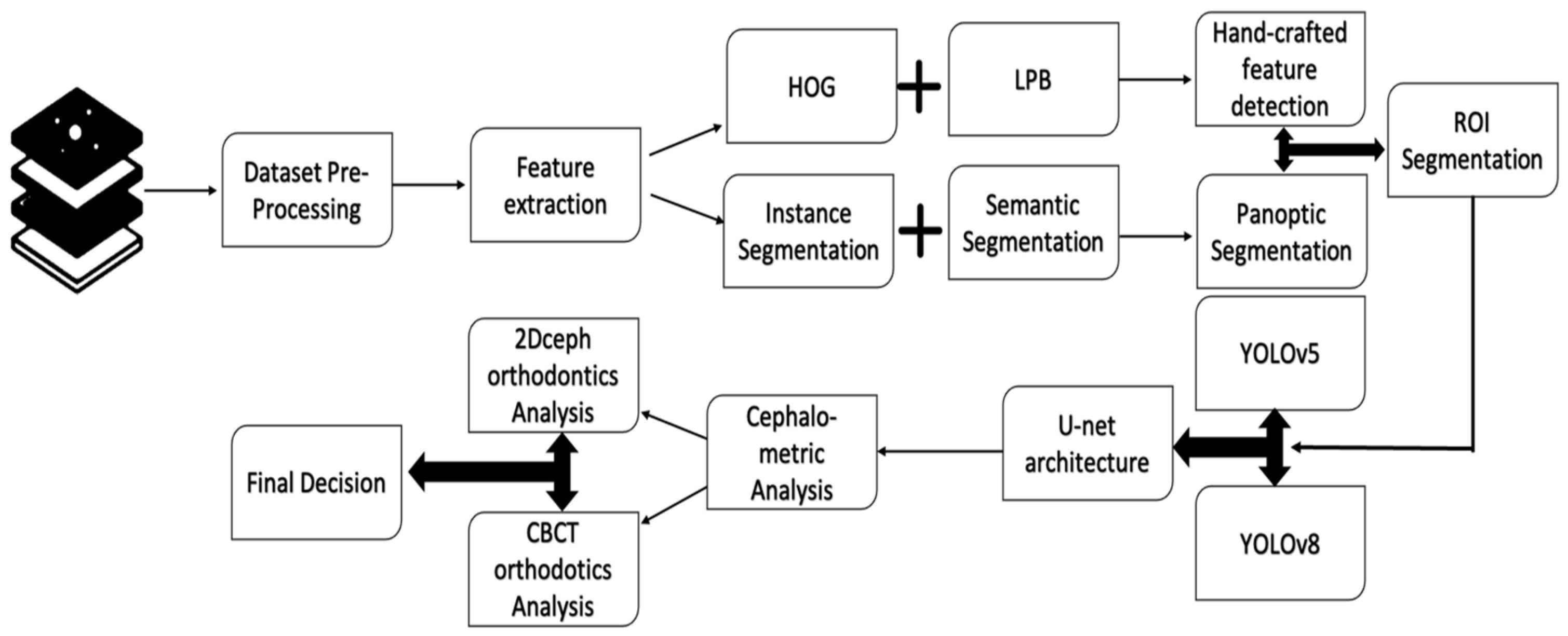
2. Materials and Methods

The proposed model shown in Figure 2 presents the YOLO-UNet model for automatic detection segmentation, comprising a serial combination of the YOLO and UNet architectures based on the integration between handcrafted features and panoptic segmentation. It begins with data preprocessing, followed by feature extraction and segmentation steps, leading to final decision-making.

2.1. Radiographic Image Enhancement and Pre-Processing Using “Local Contrast Enhancement” Technique

Ceph-X was developed by applying some image processing techniques to enhance the X-ray images, locate landmarks, and compute automatically linear and angular cephalometric measurements, as shown in Figure 3.
Local contrast enhancement (LCE) is a technique for bringing out detail and texture in an image. It is very similar to sharpening, which accentuates only fine detail, but it operates at a larger scale. LCE sometimes goes by other names such as clarity or micro-contrast. Most of the X-ray images in this work lack detail and create artifacts, which are especially seen for the digital image that is taken with an X-ray film. Therefore, X-ray images are necessarily pre-processed to derive a clearer image, for which the local contrast enhancement technique has been applied in this paper [27].
For the local contrast enhancement technique, let the intensity, f, of the picture elements (pixels) of an N × N digital image be indexed by (i,j) 1 <= i, j <= N. Consider a sub image of size M × M centered on (i, j), and denote the mean and standard deviation of the intensity within W by <f>W and σW (f), respectively. The objective of this method is to define a point transformation dependent on W such that the distribution is localized around the mean of the intensity and covers the entire intensity range, as shown in Figure 4. The implicit assumption is that W is large enough to contain a statistically representative distribution of the local variation of grey levels, yet small enough to be unaffected by the gradual change of contrast between the center and the periphery of the X-ray image. The adaptive contrast enhancement transformation is defined by
f i , j g i , j = 255 ψ w f ψ w f m i n ψ w f m a x ψ w f m i n
where the sigmoidal function is
ψ w f = 1 + e x p < f > w f σ w 1
f m a x and f m i n are the maximum and minimum values of intensity within the whole image, with
< f > w ( i , j ) = 1 M 2 ( k , l ) ϵ ( i , j ) f k , l
σ W 2 f = ( k , l ) ϵ ( i , j ) ( f k , l < f > w ) 2
  • S (sella):
  • The midpoint of the sella turcica (a saddle-shaped depression in the sphenoid bone at the base of the skull);
  • Used as a stable reference point in cephalometric analysis because it does not change much after early childhood;
  • PNS (posterior nasal spine):
  • The rearmost point of the bony hard palate (part of the roof of the mouth);
  • Important for evaluating the length and position of the maxilla (upper jaw);
  • ANS (anterior nasal spine):
  • The tip of the bony projection at the front of the upper jaw (part of the nasal cavity);
  • Helps measure facial height and the forward positioning of the maxilla;
  • Me (Menton):
  • The lowest point on the contour of the chin (mandible);
  • Essential for assessing vertical jaw relationships and facial symmetry;
  • Go (Gonion):
  • The most outward and backward point at the angle of the mandible (lower jaw);
  • Important for evaluating the mandibular plane angle and jaw growth patterns.

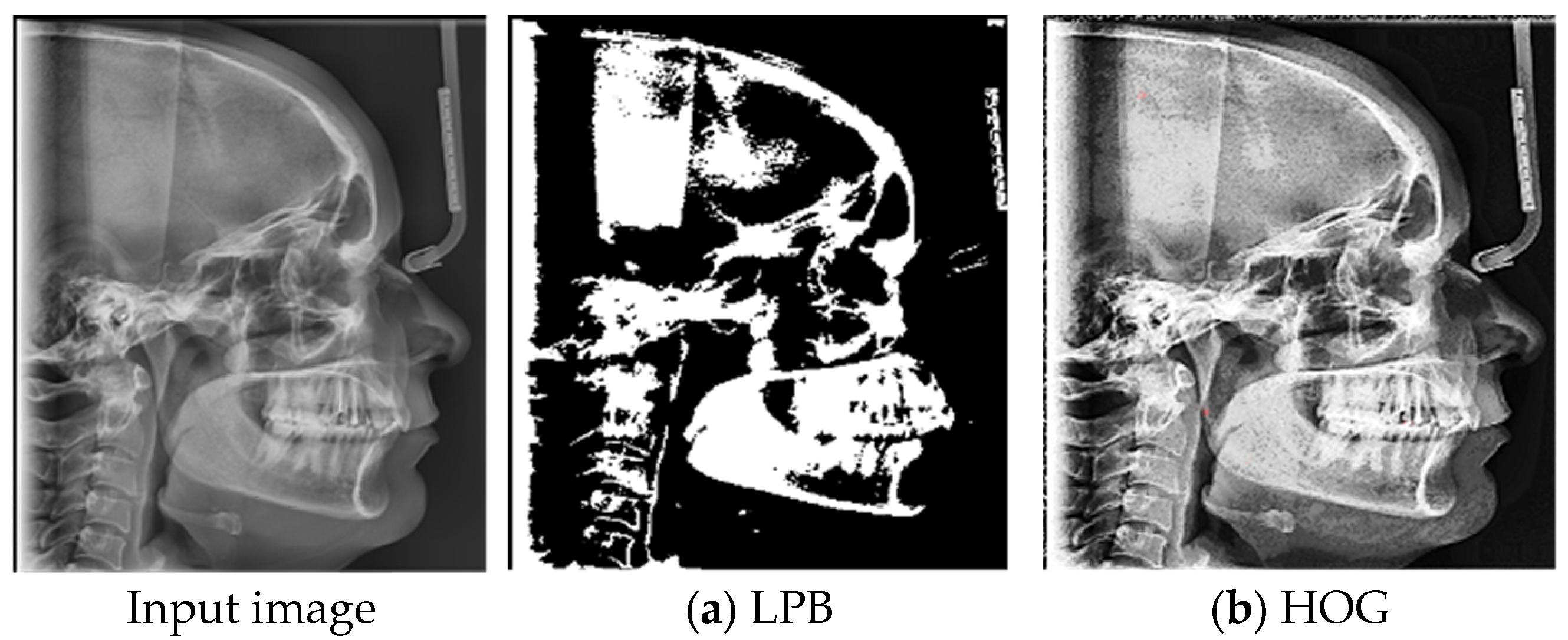
2.2. ROI Handcrafted Feature Detection

The identification of features is conducted using algorithms that describe them with vector values. The LBP and HOG feature descriptor algorithms are widely used in facial recognition applications [28,29,30,31]. LBP encodes the texture of a grayscale image by comparing the intensity differences between each pixel and its neighbors, forming a 256-dimensional feature vector as shown in Figure 5a. An advanced version, the uniform pattern LBP, addresses frequently occurring patterns. The HOG technique [28,29,30,31] as shown in Figure 5b depicts edges and corners by analyzing local intensity gradients, and generating magnitude and angle matrices, which are divided into rectangular cells. Each cell’s gradients form a nine-point histogram, creating a feature vector of size 36, as shown in Figure 5.

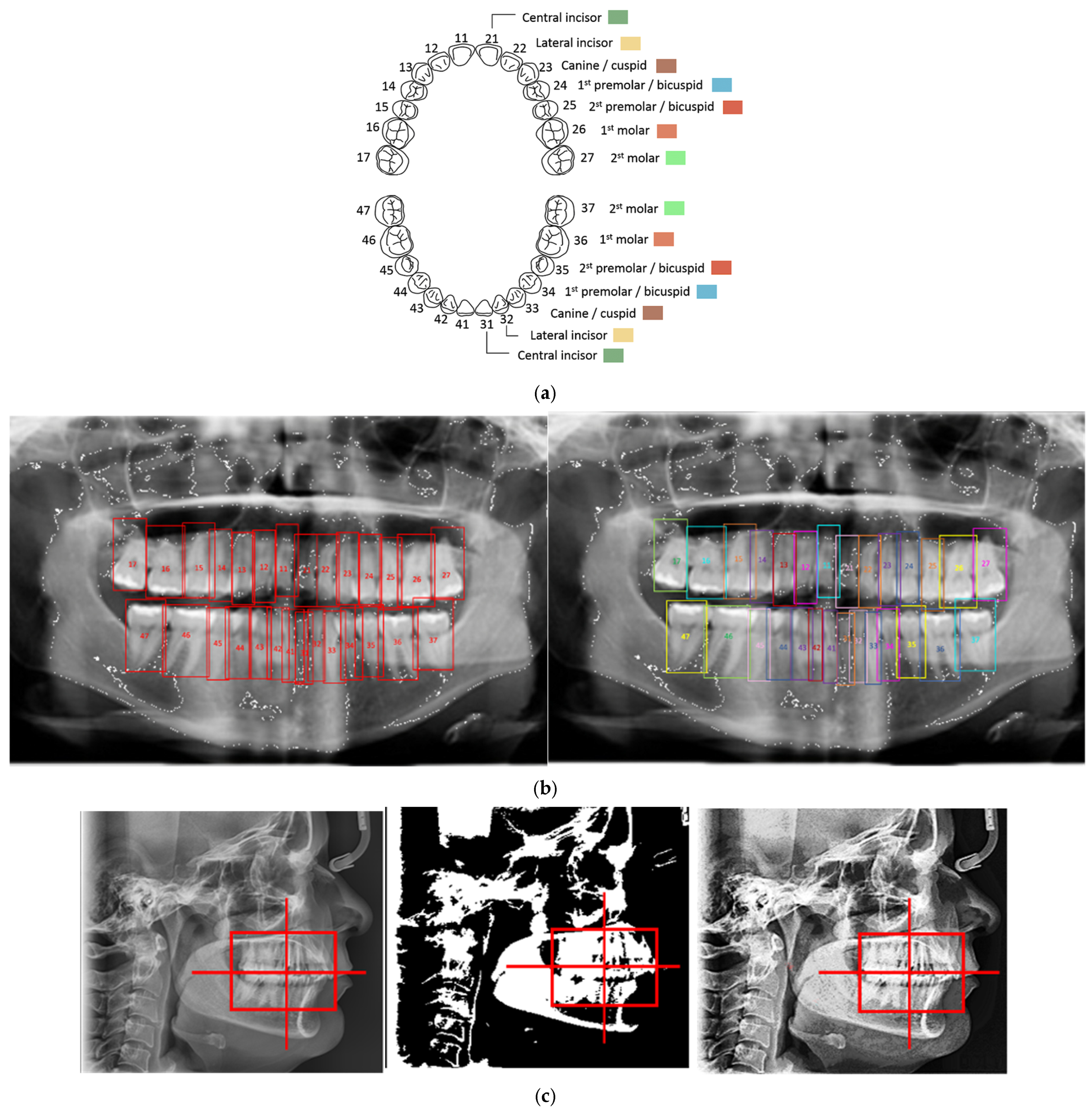
2.3. ROI Identification, YOLO-UNet-Based

In response to the recent challenge of panoptic segmentation, which involves assigning a label to every pixel in an image along with an instance ID, a new architectural design based on YOLO has been introduced for this specific task in computer vision. This design makes use of the YOLOv8 framework, incorporating parallel heads for semantic and instance segmentation to carry out comprehensive scene parsing. The results from this architecture demonstrate successful segmentation, ensuring that the boundaries between background classes align closely with the ground truth, while the instance masks accurately represent the shapes of objects in a scene.
Semantic segmentation [32] is the process of assigning each pixel in an input image to a specific class, a task that poses significant challenges in computer vision. This segmentation is essential for identifying classes at the pixel level, proving highly beneficial in applications like autonomous driving, pedestrian detection, and medical diagnosis. Deep learning, especially Convolutional Neural Networks (CNNs), has introduced various event segmentation techniques, leading to significant improvements in segmentation accuracy. The event segmentation module predicts the centroid of each event along with an offset vector originating from each foreground pixel and pointing towards the corresponding centroid.
Panoptic segmentation [33] emerges as a method to bridge the gap in understanding scenes through both semantic and instance segmentation. The fundamental idea of panoptic segmentation revolves around the comprehensive recognition and segmentation of the different components present in input images. Distinct colors are assigned to the teeth segmentation results to distinguish the segmentation outcomes. In contrast to semantic and instance segmentation, panoptic segmentation conducts a thorough visual examination of each individual element within the entire scene. This holistic approach greatly enhances the ability to comprehend the scene. Initially, the early panoptic segmentation algorithm simply combined the semantic segmentation model with the instance segmentation model to address the limitations of both techniques.
Nevertheless, an increasing understanding of the challenges presented by panoptic segmentation is needed. The combination of handcrafted feature extraction and panoptic segmentation enhances the incorporation of various deep learning techniques such as vgg16, Resnet 50, and YOLO-UNet.
The YOLO-UNet model is a fusion of YOLO and UNet architectures for automated detection and segmentation based on instance and semantic segmentation. YOLO (You Only Look Once) is a deep learning method focused on object detection, designed for real-time processing by treating objects as a single regression problem from raw image pixels to distinct spatial bounding boxes and their respective probability classes. The human brain rapidly identifies and interprets visual information. During object detection, the segmentation technique used by the current detection framework guides the classifier to a specific object, assessing it across various scales and positions in the test image. The selection of the YOLO architecture in this research is based on its speed and accuracy in detecting teeth. YOLO is integrated with the UNet architecture. YOLOv8, also referred to as Darknet-53 [34], consists of a total of 53 convolutional layers. This version of YOLO incorporates a residual block or shortcut connection that involves adding the inputs before the convolutional layer residual block, along with outcomes from a 1 × 1 convolutional layer filter followed by batch normalization and leaky ReLU, as well as a 3 × 3 convolutional layer filter with batch normalization and a final leaky ReLU. YOLOv8, an improved version of YOLOv5, excels in speed and accuracy. The YOLO-UNet approach is employed for the detection, segmentation and localization of teeth, which steps are essential in orthodontic analysis and diagnosis. A hybrid deep learning model that precisely segments the required landmark regions with UNet to enable YOLOv8s to efficiently detect, classify and localize maxilla and mandible teeth is shown in Figure 6b. Moreover, Figure 6c shows a sample of ROI detection results derived from lateral cephalometric assessment required in a preprocessing step before line tracing and analysis, which are important in orthodontics evaluations. Figure 6a shows a key chart for tooth labeling.

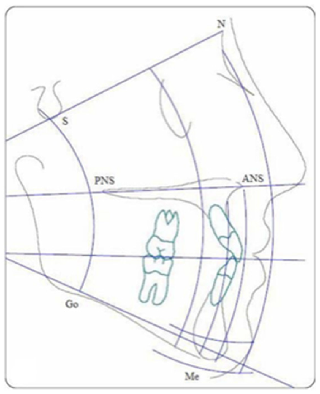
2.4. Line Tracing and Analysis Using Different AI Models

The proposed method could be used to segment the needed cephalometric landmarks of the skull and face in both bones and soft surface sections of cephalometric images using the ROI segmented in Figure 7a, using the explainable deep learning model applied on panorama radiographs. Some landmarks can be generated automatically and can be used as a guideline for locating the reference landmark using the AI model and the software shown in Figure 7b,c. The model also provides tools that allow users to mark the correct ROI with ease.
A 3D dental scan, also known as Cone-Beam Computed Tomography (CBCT), is a type of X-ray used in the dental industry. It delivers a three-dimensional image of teeth, soft tissues, nerve pathways, and bone in a single scan, revolutionizing dental care with its level of detail and precision, as shown in Figure 8a,b.
3D cephalometry is a powerful tool for measuring the skull and face in three dimensions. It offers many advantages, including providing a detailed 3D view of the skull’s hard and soft tissues, enabling 3D cephalometric analysis at real-life size (1:1 scale), avoiding the overlapping of anatomical structures and providing high accuracy and reliability. Additionally, it allows for the establishment of a 3D reference system for analyzing changes in the skull and face over time [35]. Although conventional spiral CT 3D cephalometry represents a significant advancement over conventional 2D cephalometry, it still has some drawbacks, including (1) the distortion of the position of facial soft tissues due to the horizontal positioning of the patient during imaging, (2) the limited detail of occlusion due to artifacts, (3) limited access for routine dentofacial deformity patients because of higher costs, and (4) the higher level of radiation exposure compared to other traditional plain film radiographs.
CBCT addresses many of the limitations faced in the transition from traditional 2D to 3D cephalometric analysis, necessitating the comparison of previous 2D images with the new 3D images. CBCT offers simulation tools that can fill the gap between image types. CBCT acquisitions can be made to simulate panoramic, lateral, and posteroanterior cephalometric radiographs so that they can be compared with pre-existing cephalometric databases.

3. Results

3.1. Experimental Environment

A new enhanced algorithm was verified within a distinctive environment consisting of two different datasets with diverse properties. A comprehensive range of diverse images was employed to accomplish the goal of evaluating the algorithm’s important ability to be both efficient and durable in both types of images—2D cephalometric and 3D full skull.

3.2. Dataset Description

A dataset of radiography 2D cephalometric and CBCT data of a full skull was collected from dental and maxillofacial imaging centers in Alexandria, Egypt. The CBCT data are in DICOM format. There are 7650 images in total. The dataset consists of multiple classes for 2D scans and CBCT—class 1 is for normal teeth where the maxilla and mandible are in harmony, and the bite is normal but the upper teeth slightly overlap the lower teeth; class 2 (or class II) is for malocclusions, characterized by upper molars that are too far forward compared to the lower molars, and where the maxilla shows prognathism or the mandible shows retrognathism, or both are true; Class 3 is the rarest type of malocclusion. Class 3 malocclusions arise when the lower molars are positioned excessively far forward relative to the upper molars. This occurs due to the maxilla being retrognathic, the mandible being prognathic, or both.

3.3. Results Obtained from 2D Lateral Cephalogram Analysis Applying AI Techniques

The proposed architecture employs UNet. It consists of a contracting path and an expansive path, both of which involve the repeated application of two 3 × 3 convolutions, each followed by LeakyReLU activation and either 2 × 2 max pooling (in the contracting path) or up-sampling (in the expansive path) [18]. Data augmentation was not applied on the input images to ensure that the deep learning model could learn from the original images [2]. The input images averaged 2067 × 1675 pixels, with each having a unique pixel size.
In general, the process of image segmentation involves a comprehensive description of the entire image through the extraction of features or the utilization of methods that facilitate the learning of maxilla and mandible positions. During the X-ray acquisition and transmission process, images are degraded, often with several types of noise originating from multiple sources. Thus, enhanced X-ray images are required to ensure the accuracy of the location and measurement process. Subsequently, panoptic segmentation is employed to discern the identity of the object in radiography.
In the realm of deep learning, the projection of segmentation maps for complete images is accomplished by sequentially predicting each slice while moving in several directions. The fusion of different handcrafted features aids in reaching an accurate result. In the majority of instances, the output of a neural network yields either a projected value for the relevant output factor or a set of probabilities, as in Figure 9, where we see the angle between the Gnathion and the Gonion, and Occ. refers to occlusion. Moreover, the results of angle measurement are shown in detail in Figure 10. The benefits of applying AI in orthodontics analysis were analyzed for each landmark, as shown below. These figures show the analytical tracing applied on 2D lateral cephalometric images.
After applying explainable deep learning, the results obtained are shown in Figure 10. The results were obtained by applying the proposed architecture in terms of vertical skeletal relations, sagittal skeletal relations, dento-basal relations, and dental relations. The normal values of these relations were set by the European Orthodontics Board, and the actual value is the result of the difference between the normal and the actual one. A comparison will be presented in the discussion section between this architectural analysis and the analysis performed on the Romexis version 6.4.3.33.66 platform including 2D and CBCT orthodontics analysis.

4. Discussion

The comparison of orthodontic analysis parameters between the groups revealed no significant differences in measurements. Furthermore, the intra-operator reliability, evaluated through paired T-tests, demonstrated high consistency in measurements.
The integration of technology has become a crucial element in medical and dental education, clinical research, diagnosis, and treatment planning. The rising use of dental smartphone applications by students and professionals to enrich their learning and clinical practice showcases technological advancements.
This system can be smoothly incorporated into digital workflows, enhancing the efficiency of patient management. Moreover, the data gathered from the Romexis application for cephalometric analysis can be easily stored, utilized, and retrieved as necessary, saving valuable office space typically allocated for record-keeping. The study integrated variables from a commonly used cephalometric analysis to mimic real-life situations and consistently evaluate the application’s performance. Utilizing this model as an initial step before manual tracing with any analysis software in the future will enhance results with fewer errors in a shorter time frame. However, the focus on CBCT analysis is projected to grow, as it signifies the future direction in the dental field.

4.1. Proposed Model Performance Measures

This section shows the performance measure mainly in terms of the training and validation loss and accuracy of the proposed model, and different scenarios applied to test the most reliable one. Table 1 demonstrates a comparison between different performance measures for each scenario versus model four, which is the proposed one.
Mode 1 and 2 show feature fusions between LBP and HOG with YOLOv5 and YOLOv8 Model 3, applying semantic and instance segmentation with panoptic segmentation combined with YOLOv5 and YOLOv8. Figure 11a identifies the training loss and validation loss, which are all slight for the four proposed scenarios, and Figure 11b highlights the validation and training accuracy values of the different models shown in Table 1, which increased during execution to reach 98.8%. These measures are indicators of a reasonable result, with good performance. The confusion matrix for this model is shown in Figure 12, containing the counts of predicted and true values that help in the calculation of precision. Figure 13a,b illustrates a comparison between training and validation loss and accuracy when executing versus epochs of the proposed model and the confusion matrix of the proposed architecture.
Moreover, Model 4 shows the proposed model, which integrates the handcrafted feature extraction with panoptic segmentation, deriving an enhanced result that improves the accuracy and robustness of this architecture, as shown in Figure 13, representing training and validation loss and accuracy and showing a confusion matrix of the predicted and validated results.
The heatmaps in Table 2 improve explainability by providing a clear and understandable representation of the underlying factors influencing the model’s predictions. Grad-CAM enhances model interpretability, aids in bias detection, and facilitates decision-making refinement. Moreover, it reveals the reasoning behind the deep learning model’s predictions, by highlighting important regions in the heatmap.
The table below shows heatmaps of the explainable deep-learning predictions of various categories.
Furthermore, during the testing and validation process, this model faced some challenges—mainly the presence of some carries in multiple teeth, as ROI shown in Table 3. We applied heatmaps and deep learning techniques to predict and detect these carries.

4.2. Comparison Between This Architecture and the Launched Software’s Results

Figure 14 shows the results for the patient’s actual value, derived using AI in 2D lateral cephalometric analysis, and applying the fusion between handcrafted features and instance and semantic segmentation to enhance the panoptic segmentation. Using this step as a preprocessing step to apply deep learning techniques in segmenting the ROI can enhance the operation of orthodontics analysis in linear and angular measurements. Figure 15 shows the mean value and the actual value using a previously launched software for orthodontics analysis based on the recommendations of the European Board of Orthodontics. The results obtained from different sources were approximately the same, which means that this model achieved a higher accuracy and good performance by the fusion of feature extraction and ROI segmentation in evaluation, thus potentially assisting the orthodontists in developing a treatment plan with much fewer errors in a shorter time.

4.3. Comparison Between This Architecture and Recent Software Result

Table 4 provides an advanced comparison between the proposed model and other recent models mentioned before in Reference [36], which use different models of DL and morphological pre-processing for diverse image analysis. The table includes models tested on various datasets and a large number of images under different conditions.

4.4. CBCT Analysis Discussion

Cephalometric tracings were performed using 3D CBCT imaging to ensure accurate and comprehensive orthodontic assessment. The full-skull cephalometric scans, provided in DICOM format, were processed using the Romexis software version 6.4.3.33.66 by Planmeca, which supports detailed 3D analysis. Before starting the analysis, the images were calibrated using a standardized scale to ensure precise measurements. Key skeletal and dental landmarks—including Condylion Left (CoL), Condilyon Right (CoL), Nasion (N), Anterior Nasal Spine (ANS), Posterior Nasal Spine (PNS), Menton (Me), and Gonion (Go), as shown in Figure 16a—were carefully identified, as they are also used in conventional 2D cephalometry. These landmarks served as reference points for calculating linear and angular measurements in accordance with the European Board of Orthodontics guidelines. After identifying all necessary points, the software automatically computed critical measurements, which were thoroughly recorded for evaluation. This process not only facilitated the accurate documentation of the patient’s cephalometric profile, but also helped determine their skeletal classification, and supported clinical diagnosis and treatment planning, as shown in Figure 16b.
In CBCT-based orthodontic analysis, skeletal and dental classifications serve different but complementary purposes. Skeletal classification focuses on the positions and relationships of the jaws (maxilla and mandible) within the facial structure, helping to identify underlying bone discrepancies like Class I (normal), Class II (returned mandible), or Class III (protruded mandible). Dental classification, on the other hand, examines how the upper and lower teeth align and occlude, assessing bite patterns and crowding. While skeletal analysis reveals the bone foundation, dental classification shows how the teeth fit within that structure. Together, they provide a more complete understanding of the patient’s orthodontic needs.
A comprehensive statistical analysis served as the reference landmark for this framework, maintaining a 99% accuracy level. Following the initial measurements, a significant portion of the available radiographs was randomly selected for repetition with various models, including the proposed model, 2D lateral cephalometric analysis, and CBCT analysis tracing software. This was done to evaluate the performance of the suggested framework and explore the potential transition from 2D to 3D analysis, as well as update the number of ROI utilized in the orthodontic evaluation.

5. Conclusions

The application of explainable deep learning models presents a promising approach for the early detection of dental misalignment. The findings demonstrate that the model is highly reliable, effectively identifying key regions of interest (ROI) during the prediction stage.
Despite its potential, this study faced challenges related to tooth positioning, variations in size, anatomical location, overlapping structures, and interproximal gaps, all of which complicate the detection process. One of the primary research limitations involves localization accuracy, which remains a critical aspect of improving model performance. Future advancements in automatic classification and segmentation techniques may address these challenges, leading to more robust and precise diagnostic tools. Opportunities exist for enhancing automatic classification and segmentation using updated methods with better performance.
The Grad-CAM method was used to generate heatmaps to visualize the regions upon which the model focused during the decision phase. The proposed model facilitates automated detection and segmentation, reducing the number of landmarks required for orthodontic analysis while improving diagnostic precision. By minimizing human error in landmark identification, it streamlines orthodontic evaluations. The UNet architecture, known for its pixel-wise prediction capabilities, further enhances localization accuracy, demonstrating strong performance across various biomedical segmentation applications. Among the tested models, the YOLOv8-UNet architecture achieved superior results, with an impressive accuracy of 0.99 and precision of 0.98, outperforming other models by an average improvement of 0.087. Additionally, the integration of CBCT optimizes diagnostic accuracy and treatment planning in orthodontics. Moreover, the confusion matrix shows how well the model classified four categories: Maxilla, Mandible, Occlusion, and No Teeth.
The explainable deep learning techniques have the power to improve diagnosis and treatment planning in orthodontics, and could be used in conjunction with other diagnostic tools to provide a more comprehensive assessment of dental health; also, they should be compared with other available platforms on the market to evaluate differences in accuracy, performance, and efficiency.

Author Contributions

Conceptualization, L.A.A., S.M.Y. and M.N.E.; Methodology, L.A.A. and S.M.Y.; Validation, L.A.A.; Formal analysis, L.A.A.; Resources, L.A.A.; Writing—review & editing, L.A.A. and S.M.Y.; Supervision, S.M.Y. and S.M.E.-S. All authors have read and agreed to the published version of the manuscript.

Funding

This research received no external funding.

Institutional Review Board Statement

This research was under the supervision of Sherin M. Youssef, who has reviewed the research protocol, including the study design, informed consent documents, recruitment materials, and data management plan. Moreover, Sahar M. El-Sheikh was the medical expert during the whole study. This study has been reviewed and determined to pose no ethical concerns. All procedures comply with established ethical guidelines and ensure participant safety and confidentiality.

Informed Consent Statement

Informed consent was obtained from all subjects involved in the study.

Data Availability Statement

Data collected from different patient with an informed consent.

Conflicts of Interest

The authors declare no conflict of interest.

References

  1. MarketsandMarkets. Artificial Intelligence (AI) in Healthcare Market Worth $148.4 Billion by 2029—Exclusive Report by MarketsandMarketsTM; PR Newswire: New York, NY, USA, 2024. [Google Scholar]
  2. Meade, M.J.; Dreyer, C.W. Tooth agenesis: An overview of diagnosis, aetiology and management. Jpn. Dent. Sci. Rev. 2023, 59, 209–218. [Google Scholar] [CrossRef] [PubMed] [PubMed Central]
  3. Grahnen, H. Hypodontia in the permanent dentition: A clinical and genetical investigation. Odont. Revy 1956, 7, 1–100. [Google Scholar]
  4. Neela, P.K.; Atteeri, A.; Mamillapalli, P.K.; Sesham, V.M.; Keesara, S.; Chandra, J.; Monica, U.; Mohan, V. Genetics of dentofacial and orthodontic abnormalities. Glob. Med. Genet. 2020, 7, 95–100. [Google Scholar] [CrossRef] [PubMed] [PubMed Central]
  5. Lee, H.; Cho, J.M.; Ryu, S.; Ryu, S.; Chang, E.; Jung, Y.S.; Kim, J.Y. Automatic identification of posteroanterior cephalometric landmarks using a novel deep learning algorithm: A comparative study with human experts. Sci. Rep. 2023, 13, 15506. [Google Scholar] [CrossRef] [PubMed] [PubMed Central]
  6. Kazimierczak, W.; Wajer, R.; Wajer, A.; Kiian, V.; Kloska, A.; Kazimierczak, N.; Janiszewska-Olszowska, J.; Serafin, Z. Periapical lesions in panoramic radiography and CBCT imaging—Assessment of AI’s diagnostic accuracy. J. Clin. Med. 2024, 13, 2709. [Google Scholar] [CrossRef]
  7. Dipalma, G.; Inchingolo, A.D.; Inchingolo, A.M.; Piras, F.; Carpentiere, V.; Garofoli, G.; Azzollini, D.; Campanelli, M.; Paduanelli, G.; Palermo, A.; et al. Artificial intelligence and its clinical applications in orthodontics: A systematic review. Diagnostics 2023, 13, 3677. [Google Scholar] [CrossRef]
  8. Surendran, A.; Daigavane, P.; Shrivastav, S.; Kamble, R.; Sanchla, A.D.; Bharti, L.; Shinde, M. The future of orthodontics: Deep learning technologies. Cureus 2024, 16, e62045. [Google Scholar] [CrossRef] [PubMed] [PubMed Central]
  9. MedlinePlus. Understanding Genetics: What Is a Gene? Available online: https://medlineplus.gov/genetics/understanding/basics/gene/ (accessed on 11 May 2025).
  10. Cleveland Clinic. Malocclusion. Available online: https://my.clevelandclinic.org/health/diseases/22010-malocclusion (accessed on 11 May 2025).
  11. Watted, N.; Lone, I.M.; Midlej, K.; Zohud, O.; Awadi, O.; Masarwa, S.; Watted, A.; Paddenberg, E.; Krohn, S.; Kirschneck, C.; et al. The complexity of skeletal transverse dimension: From diagnosis, management, and treatment strategies to the application of Collaborative Cross (CC) mouse model. J. Funct. Morphol. Kinesiol. 2024, 9, 51. [Google Scholar] [CrossRef] [PubMed] [PubMed Central]
  12. CephX. Comparison of 2D and 3D Cephalometric Analyses. Available online: https://cephx.com/comparison-2d-3d-cephalometric-analyses-2/ (accessed on 11 May 2025).
  13. Baldini, B.; Cavagnetto, D.; Baselli, G.; Sforza, C.; Tartaglia, G.M. Cephalometric measurements performed on CBCT and reconstructed lateral cephalograms: A cross-sectional study providing a quantitative approach of differences and bias. BMC Oral Health 2022, 22, 98. [Google Scholar] [CrossRef]
  14. Hage, L.; Kmeid, R.; Amm, E. Comparison between 2D cephalometric and 3D digital model superimpositions in patients with lateral incisor agenesis treated by canine substitution. Am. J. Orthod. Dentofac. Orthop. 2024, 165, 93–102. [Google Scholar] [CrossRef]
  15. Rossini, G.; Cavallini, C.; Cassetta, M.; Barbato, E. 3D cephalometric analysis obtained from computed tomography. Review of the literature. Ann. Stomatol. 2011, 2, 31–39. [Google Scholar]
  16. Abdelkarim, A. Cone-beam computed tomography in orthodontics. Dent. J. 2019, 7, 89. [Google Scholar] [CrossRef] [PubMed]
  17. Porto, L.F.; Lima, L.N.C.; Flores, M.R.P.; Valsecchi, A.; Ibanez, O.; Palhares, C.E.M.; Vidal, F.D.B. Automatic Cephalometric Landmarks Detection on Frontal Faces: An Approach Based on Supervised Learning Techniques. Digit. Investig. 2019, 30, 108–116. [Google Scholar] [CrossRef]
  18. Sharpe, P.T. Homeobox genes and orofacial development. Connect. Tissue Res. 1995, 32, 17–25. [Google Scholar] [CrossRef]
  19. Nakasima, A.; Ichinose, M.; Nakata, S.; Takahama, Y. Hereditary factors in the craniofacial morphology of Angle’s Class II and Class III malocclusions. Am. J. Orthod. 1982, 82, 150–156. [Google Scholar] [CrossRef]
  20. De Coster, P.J.; Marks, L.A.; Martens, L.C.; Huysseune, A. Dental agenesis: Genetic and clinical perspectives. J. Oral Pathol. Med. 2009, 38, 1–17. [Google Scholar] [CrossRef]
  21. Kazimierczak, N.; Kazimierczak, W.; Serafin, Z.; Nowicki, P.; Nożewski, J.; Janiszewska-Olszowska, J. AI in orthodontics: Revolutionizing diagnostics and treatment planning—A comprehensive review. J. Clin. Med. 2024, 13, 344. [Google Scholar] [CrossRef]
  22. Rauniyar, S.; Jena, S.; Sahoo, N.; Mohanty, P.; Dash, B.P. Artificial intelligence and machine learning for automated cephalometric landmark identification: A meta-analysis previewed by a systematic review. Cureus 2023, 15, e40934. [Google Scholar] [CrossRef]
  23. Kunz, F.; Stellzig-Eisenhauer, A.; Widmaier, L.M.; Zeman, F.; Boldt, J. Assessment of the quality of different commercial providers using artificial intelligence for automated cephalometric analysis compared to human orthodontic experts. Untersuchung der Auswertequalität kommerzieller Anbieter für KI-basierte FRS Analysen im Vergleich zu einem Experten-Goldstandard. J. Orofac. Orthop. 2023, 86, 145–160. [Google Scholar] [CrossRef]
  24. Durão, A.R.; Pittayapat, P.; Rockenbach, M.I.; Olszewski, R.; Ng, S.; Ferreira, A.P.; Jacobs, R. Validity of 2D lateral cephalometry in orthodontics: A systematic review. Prog. Orthod. 2013, 14, 31. [Google Scholar] [CrossRef]
  25. Alsubai, S. A Critical Review on the 3D Cephalometric Analysis Using Machine Learning. Computers 2022, 11, 154. [Google Scholar] [CrossRef]
  26. Park, J.-H.; Hwang, H.-W.; Moon, J.-H.; Yu, Y.; Kim, H.; Her, S.-B.; Srinivasan, G.; Aljanabi, M.N.A.; Donatelli, R.E.; Lee, S.-J. Automated identification of cephalometric landmarks: Part 1—Comparisons between the latest deep-learning methods YOLOV3 and SSD. Angle Orthod. 2019, 89, 903–909. [Google Scholar] [CrossRef] [PubMed]
  27. Cambridge in Colour. Local Contrast Enhancement. Available online: https://www.cambridgeincolour.com/tutorials/local-contrast-enhancement.htm (accessed on 11 May 2025).
  28. Mady, H.; Hilles, S.M.S. Face recognition and detection using Random forest and combination of LBP and HOG features. In Proceedings of the 2018 International Conference on Smart Computing and Electronic Enterprise (ICSCEE), Shah Alam, Malaysia, 11–12 July 2018; pp. 1–7. [Google Scholar] [CrossRef]
  29. Mirjalili, F.; Hardeberg, J.Y. On the quantification of visual texture complexity. J. Imaging 2022, 8, 248. [Google Scholar] [CrossRef]
  30. Pan, Z.; Li, Z.; Fan, H.; Wu, X. Feature based local binary pattern for rotation invariant texture classification. Expert Syst. Appl. 2017, 88, 238–248. [Google Scholar] [CrossRef]
  31. Analytics Vidhya. Feature Engineering for Images—Introduction to HOG Feature Descriptor. Available online: https://www.analyticsvidhya.com/blog/2019/09/feature-engineering-images-introduction-hog-feature-descriptor/ (accessed on 11 May 2025).
  32. Pareto, A.I. Semantic Segmentation. Available online: https://pareto.ai/blog/semantic-segmentation (accessed on 11 May 2025).
  33. Kirillov, A.; He, K.; Girshick, R.; Rother, C.; Dollar, P. Panoptic segmentation. In Proceedings of the 2019 IEEE/CVF Conference on Computer Vision and Pattern Recognition (CVPR), Long Beach, CA, USA, 15–20 June 2019; pp. 9396–9405. [Google Scholar] [CrossRef]
  34. Hussain, M. YOLO-v1 to YOLO-v8, the rise of YOLO and its complementary nature toward digital manufacturing and industrial defect detection. Machines 2023, 11, 677. [Google Scholar] [CrossRef]
  35. Qian, Y.; Qiao, H.; Wang, X.; Zhan, Q.; Li, Y.; Zheng, W.; Li, Y. Comparison of the accuracy of 2D and 3D cephalometry: A systematic review and meta-analysis. Australas. Orthod. J. 2022, 38, 130–144. [Google Scholar] [CrossRef]
  36. Ashame, L.A.; Youssef, S.M.; ElAgamy, M.N.; El-Sheikh, S.M. An enhanced assistive model for diagnosis of dental 3D panoramic radiographs integrating the fusion of handcrafted features with deep learning architectures. In Proceedings of the 2024 International Conference on Machine Intelligence and Smart Innovation (ICMISI), Alexandria, Egypt, 12–14 May 2024; pp. 272–277. [Google Scholar] [CrossRef]
  37. Oktay, A.B. Tooth detection with convolutional neural networks. In Proceedings of the 2017 Medical Technologies National Conference (TIPTEKNO), Trabzon, Turkey, 12–14 October 2017; pp. 1–4. [Google Scholar] [CrossRef]
  38. Yang, J.; Xie, Y.; Liu, L.; Xia, B.; Cao, Z.; Guo, C. Automated dental image analysis by deep learning on small dataset. In Proceedings of the 2018 IEEE 42nd Annual Computer Software and Applications Conference (COMPSAC), Tokyo, Japan, 3–27 July 2018; pp. 492–497. [Google Scholar] [CrossRef]
  39. Zhang, K.; Wu, J.; Chen, H.; Lyu, P. An effective teeth recognition method using label tree with cascade network structure. Comput. Med. Imaging Graph. 2018, 68, 61–70. [Google Scholar] [CrossRef]
  40. Singh, N.K.; Raza, K. Progress in Deep Learning-Based Dental and Maxillofacial Image Analysis: A Systematic Review. Expert Syst. Appl. 2022, 199, 116968. [Google Scholar] [CrossRef]
  41. Muramatsu, C.; Morishita, T.; Takahashi, R.; Hayashi, T.; Nishiyama, W.; Ariji, Y.; Zhou, X.; Hara, T.; Katsumata, A.; Ariji, E.; et al. Tooth detection and classification on panoramic radiographs for automatic dental chart filing: Improved classification by multi-sized input data. Oral Radiol. 2021, 37, 13–19. [Google Scholar] [CrossRef]
  42. Tuzoff, D.V.; Tuzova, L.N.; Bornstein, M.M.; Krasnov, A.S.; Kharchenko, M.A.; Nikolenko, S.I.; Sveshnikov, M.M.; Bednenko, G.B. Tooth detection and numbering in panoramic radiographs using convolutional neural networks. Dentomaxillofac. Radiol. 2019, 48, 20180051. [Google Scholar] [CrossRef]
  43. Laishram, A.; Thongam, K. Detection and classification of dental pathologies using faster-RCNN in orthopantomogram radiography image. In Proceedings of the 2020 7th International Conference on Signal Processing and Integrated Networks (SPIN), Noida, India, 27–28 February 2020; IEEE: Piscataway, NJ, USA; pp. 423–428. [Google Scholar]
  44. Eun, H.; Kim, C. Oriented tooth localization for periapical dental X-ray images via convolutional neural network. In Proceedings of the 2016 Asia-Pacific Signal and Information Processing Association Annual Summit and Conference (APSIPA), Jeju, Republic of Korea, 13–15 December 2016. [Google Scholar] [CrossRef]
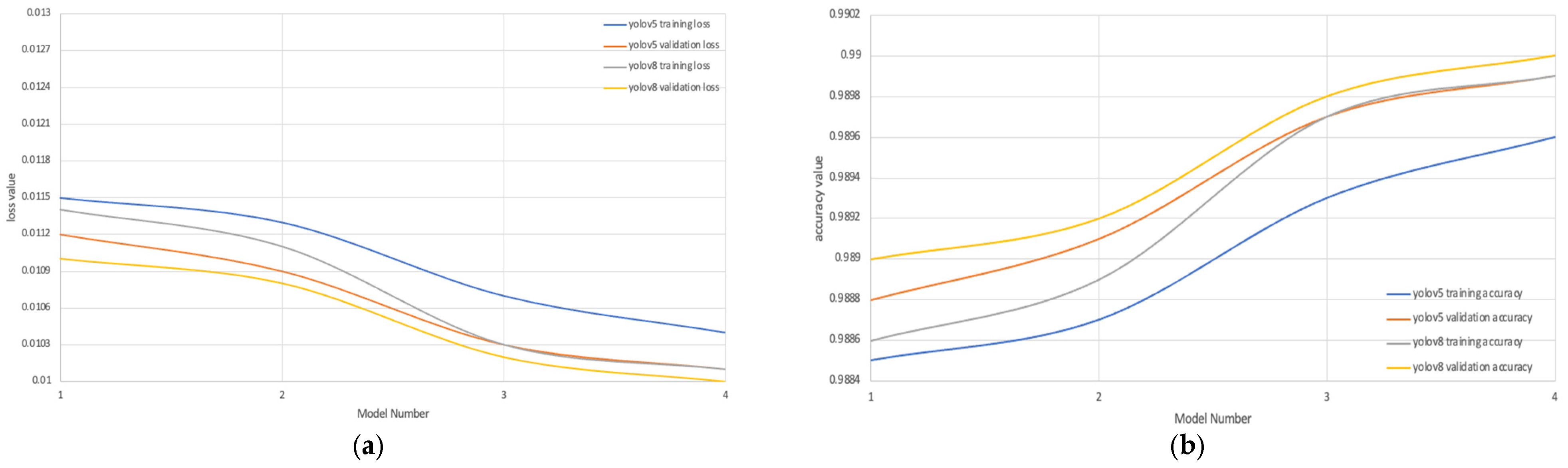
Figure 1. (a) Class 1: Normal jaw alignment with a balanced bite. Class 2: The upper jaw (maxilla) is positioned forward-which is shown by the blue arrow—relative to the lower jaw (mandible), often leading to an overbite. Class 3: The lower jaw is positioned forward relative to the upper jaw-which is shown by the blue arrow, resulting in an underbite, moreover the dashed line to facilitate showing the miss-alignmet between the maxilla and mandible (b) Sample of 2D lateral cephalometric of malocclusion “bad bite” and its line tracing after analysis.
Computers 14 00223 g001
Figure 2. Proposed model representing the integration between handcrafted features and the panoptic segmentation for the ROI of 2D cephalometric and CBCT analyses.
Computers 14 00223 g002
Figure 3. Main angles and landmarks needed in 2D lateral cephalometric analysis.
Computers 14 00223 g003
Figure 4. The result of the local contrast enhancement technique followed by the input image.
Computers 14 00223 g004
Figure 5. The result obtained from applying LPB (a) and HOG (b) on the input lateral ceph.
Computers 14 00223 g005
Figure 6. (a) Key chart for tooth labeling where each teeth has his own number and each corresponding couple of tooth have the same color to be more clear to understand. (b) ROI detection in a panorama radiograph using an AI model based on the deep learning architecture; figure showing teeth labeling in panoramic radiographs. (c) Sample of ROI detection results from a lateral cephalometric.
Computers 14 00223 g006
Figure 7. (a) ROI segmentation in panorama radiographs using the AI model for teeth labeling. Key chart for tooth labeling where each teeth has his own number and each corresponding couple of tooth have the same color to be more clear to understand appeard previously in Figure 6a. (b) Cephalometric line tracing for orthodontic analysis using the explainable deep learning model. (c) Cephalometric line tracing for orthodontic analysis using the previously launched software. (d) The most important landmark needed in orthodontics tracing used in Figure 7b,c tracing.
Computers 14 00223 g007aComputers 14 00223 g007b
Figure 8. (a) Layout of CBCT and different layers from the DICOM File. (b) CBCT line tracing for orthodontic analysis. CBCT landmarks are crucial for analyzing craniofacial relationships, growth patterns, and treatment planning. Several anatomical landmarks are used for cephalometric analysis. While the exact list of points may vary depending on the analysis type, here are some commonly used landmarks: Nasion (N)—The midpoint of the frontonasal suture. Sella (S)—The center of the sella turcica (pituitary fossa). A Point (Subspinale)—The deepest point on the anterior maxilla. B Point (Supramentale)—The deepest point on the anterior mandible. Pogonion (Pog)—The most anterior point on the chin. Gnathion (Gn)—The midpoint between Pogonion and Menton. Menton (Me)—The lowest point on the mandibular symphysis. Orbitale (Or)—The lowest point on the inferior orbital rim. Porion (Po)—The uppermost point on the external auditory meatus. Anterior Nasal Spine (ANS)—The tip of the anterior nasal spine. Posterior Nasal Spine (PNS)—The tip of the posterior nasal spine. Incisor Apex and Tip—Points on the upper and lower incisors for dental analysis. Gonion (Go)—The most posterior-inferior point on the angle of the mandible.
Computers 14 00223 g008
Figure 9. (a) Result of 2D line tracing using different deep learning techniques. (b) Result of 2D line tracing using the previously launched software.
Computers 14 00223 g009
Figure 10. Results obtained by applying the proposed model. (a) The sagittal skeletal relations, which include the maxillary and mandibular position and the sagittal jaw relation in terms of the normal value versus the actual value and their difference. Sagittal skeletal relation refers to the alignment of the upper and lower jaws in the front-to-back (anterior-posterior) direction. It is a key factor in orthodontics and craniofacial development, influencing bite, facial profile, and jaw function. (b) The vertical skeletal relations, which include maxillary and mandibular inclination and the vertical jaw relation in terms of normal value versus the actual value and their difference. Vertical skeletal relation refers to the up-and-down (superior-inferior) alignment of the upper and lower jaws. It plays a crucial role in determining facial height, bite function, and the overall harmony of the maxillofacial complex. This relationship is typically categorized into three types, as follows: Normal (Balanced) Vertical Relationship—The jaws and teeth align properly, maintaining a well-proportioned facial height. Increased Vertical Dimension (Long Face Syndrome) and Decreased Vertical Dimension (Short Face Syndrome)—Reduced lower facial height, which may contribute to deep bites or strong jaw compression. (c) The dental relations, which include overjet, overbite and their interincisal angle in terms of normal value versus the actual value and their difference. Dental relations refer to the way upper and lower teeth interact in terms of alignment, bite, and overall function, playing a crucial role in oral health, chewing efficiency, and facial aesthetics. These relations are classified into three dimensions: sagittal (anterior-posterior), which determines whether a person has a normal bite, an overbite (Class II), or an underbite (Class III); vertical, which assesses open bites, deep bites, or normal bites based on the vertical overlap of teeth; and transverse, which evaluates crossbites or midline shifts to ensure proper alignment from side to side. Understanding these relationships allows for precise orthodontic diagnosis and treatment planning to promote balanced function and long-term stability. (d) The dento-basal relations consist of maxillary incisor and mandibular incisor inclination and their compensation in terms of normal value versus the actual value and their difference. Dento-basal relations refer to the connection between the teeth and their supporting basal bone structures, particularly in terms of alignment, stability, and overall function. This relationship is crucial in orthodontics and prosthodontics, as it influences the positioning of teeth within the jawbone, impacting occlusion, facial aesthetics, and long-term oral health. Proper dento-basal harmony ensures efficient load distribution during chewing, and helps maintain a balanced skeletal and dental framework. Understanding these relations aids in designing orthodontic treatments and prosthetic solutions that enhance both functional and structural integrity.
Computers 14 00223 g010
Figure 11. Curves of training and validation loss and accuracy of different scenarios applied: (a) training and validation loss curve of different applied scenarios; (b) training and validation accuracy curve of different applied scenarios.
Computers 14 00223 g011
Figure 12. Confusion matrix of three applied scenarios in (a) model 1, (b) model 2 and (c) model 3, where the true value is on the y-axis and the predicted value is on the x-axis.
Computers 14 00223 g012
Figure 13. The accuracies of different epochs during the execution of the proposed architecture. (a) The training and validation loss of model four, which is the proposed architecture. The training and validation loss steadily decrease in the initial ~60 epochs, indicating effective learning and model improvement. However, between epochs 60 and 70, the validation loss begins to flatten or slightly increase, while training loss continues to decline, suggesting potential overfitting, where the model performs well on training data but loses its generalization ability for unseen data. Although the gap between training and validation loss remains relatively small, mild overfitting is present. Given this trend, an early stopping point around epoch 60–70 may be beneficial to prevent unnecessary overfitting. Implementing regularization techniques or early stopping can further enhance the model’s ability to maintain generalizability and optimize performance. (b) The training and validation accuracy during execution versus epochs. In the initial ~60 epochs, both training and validation loss steadily decrease, indicating effective learning and model improvement. However, between epochs 60 and 70, the validation loss begins to flatten or slightly increase, while training loss continues to decline, suggesting potential overfitting—where the model performs well on training data but loses generalization ability for unseen data. Although the gap between training and validation loss remains relatively small, mild overfitting is present. Given this trend, an early stopping point around epochs 60–70 may be beneficial to prevent unnecessary overfitting. Implementing regularization techniques or early stopping can further enhance the model’s ability to maintain generalizability and optimize performance. (c) The confusion matrix of the proposed architecture that implements the predicted and truth values obtained, where the truth is on the y-axis and the predicted value is on the x-axis. The model demonstrates high accuracy, with strong diagonal values for Maxilla (480), Mandible (450), and No Teeth (482), confirming its effectiveness. However, minor misclassifications occur; notably, 63 occlusion samples are classified as mandible and 30 mandible samples are misclassified as maxilla, likely due to anatomical overlap or visual similarities. Despite these small errors, overall performance remains robust, with the No Teeth category achieving perfect classification (482/482). Minor refinements or additional data may further enhance accuracy, particularly in differentiating between mandible and occlusion classes.
Computers 14 00223 g013
Figure 14. Graph for orthodontics analysis using the explainable deep learning results, showing the accuracy of the mean and current values of the accurate measurements and inclination versus the difference achieved using the proposed techniques based on the recommendations of the European Board of Orthodontics.
Computers 14 00223 g014
Figure 15. Graph for orthodontics analysis using the AI platform, showing the accuracy of the mean and current values of the accurate measurements and inclination versus the difference achieved using the proposed techniques based on the recommendations of the European Board of Orthodontics, achieved using a previously launched AI platform.
Computers 14 00223 g015
Figure 16. (a) CBCT landmarks’ identification. (b) CBCT analysis result and final decision.
Computers 14 00223 g016
Table 1. The training and validation loss and accuracy of different applied scenarios.
YOLOv5YOLOv8
Training LossTraining AccuracyValidation LossValidation AccuracyTraining LossTraining AccuracyValidation LossValidation Accuracy
Model 1 LBP0.02150.97850.02120.97880.01140.98860.0110.989
Model 2 HOG0.02130.97870.02090.97910.01110.98890.01080.9892
Model 3 Segmentation0.01070.98930.01030.98970.01030.98970.01020.9898
Model 4 Proposed Model0.01040.98960.01010.98990.01010.98990.010.99
Table 2. Applied heatmaps that predict the ROI of the explainable deep learning approach.
ClassOriginalYolov5Yolov8Mean Deviation
Class 1Computers 14 00223 i001Computers 14 00223 i002Computers 14 00223 i003Computers 14 00223 i004
Class 2Computers 14 00223 i005Computers 14 00223 i006Computers 14 00223 i007Computers 14 00223 i008
Class 3Computers 14 00223 i009Computers 14 00223 i010Computers 14 00223 i011Computers 14 00223 i012
Table 3. The results of applying heatmaps in carries prediction and the resulting confusion matrix.
OriginalPredict PhaseHeat MapsConfusion Matrix
Computers 14 00223 i013Computers 14 00223 i014Computers 14 00223 i015Computers 14 00223 i016
Computers 14 00223 i017Computers 14 00223 i018Computers 14 00223 i019
Table 4. Comparison between models used in recent research and the proposed model.
AuthorsMethodRemarkEvaluation
(Oktay, 2017) [37]CNN AlexNetCNN and AlexNet used for tooth detection and classificationAcc = 0.943,
(Yang et al., 2018) [38]CNNCNN on small dataset for automated diagnosis Pre = 0.756,
(Zhang et al., 2018) [39]CNNCNN-based cascade network used to identify tooth loss, filled and decayPr = 0.958,
(Singh et al., 2022) [40]CNNCNN-based UNet employed to segment mandibuletraining = 0.768,
validation = 0.805
(Muramatsu et al., 2020) [41]CNN
Res-Net
Res-net with CNN, a small size of imageAcc for cnn = 0.932,
Acc for Resnet = 0.98
(Tuzoff et al., 2019) [42]CNNFaster region-based CNN approach, moderate dataset sizePr = 0.994
(Laishram & Thongam, 2020) [43]CNNFaster region-based CNN applied for tooth detection and classification Detection Acc = 0.910, Classification = 0.99
(Eun & Kim, 2017) [44]CNNCNN; teeth localizationAcc = 0.90
This proposed modelFusion between handcrafted features and segmentation based on YOLO-UNetDifferent experimental scenarios employed to test the performance of the proposed modelACC = 0.99
Pre = 0.98
Avg. improvement = 0.087
Disclaimer/Publisher’s Note: The statements, opinions and data contained in all publications are solely those of the individual author(s) and contributor(s) and not of MDPI and/or the editor(s). MDPI and/or the editor(s) disclaim responsibility for any injury to people or property resulting from any ideas, methods, instructions or products referred to in the content.

