Pain Level Classification Using Eye-Tracking Metrics and Machine Learning Models

Abstract

Pain estimation is a critical aspect of healthcare, particularly for patients who are unable to communicate discomfort effectively. The traditional methods, such as self-reporting or observational scales, are subjective and prone to bias. This study proposes a novel system for non-invasive pain estimation using eye-tracking technology and advanced machine learning models. The methodology begins with preprocessing steps, including resizing, normalization, and data augmentation, to prepare high-quality input face images. DeepLabV3+ is employed for the precise segmentation of the eye and face regions, achieving 95% accuracy. Feature extraction is performed using VGG16, capturing key metrics such as pupil size, blink rate, and saccade velocity. Multiple machine learning models, including Random Forest, SVM, MLP, XGBoost, and NGBoost, are trained on the extracted features. XGBoost achieves the highest classification accuracy of 99.5%, demonstrating its robustness for pain level classification on a scale from 0 to 5. The feature analysis using SHAP values reveals that pupil size and blink rate contribute most to the predictions, with SHAP contribution scores of 0.42 and 0.35, respectively. The loss curves for DeepLabV3+ confirm rapid convergence during training, ensuring reliable segmentation. This work highlights the transformative potential of combining eye-tracking data with machine learning for non-invasive pain estimation, with significant applications in healthcare, human–computer interaction, and assistive technologies.

1. Introduction

1.1. Context

Accurate pain estimation is a cornerstone of effective patient care, particularly in contexts where individuals are unable to communicate their discomfort, such as in intensive care units (ICUs), pediatric care, or among non-verbal patients with cognitive impairments or severe disabilities [1]. Traditional assessment tools—such as the Visual Analog Scale (VAS) or the Behavioral Pain Scale (BPS)—rely heavily on subjective self-reporting or observation [2]. While useful, these approaches are prone to bias and fail to provide real-time, objective, or continuous monitoring, which are critical in clinical environments requiring timely interventions.

Advancements in computer vision and machine learning have enabled non-invasive approaches to pain estimation by analyzing physiological and behavioral signals [3], including facial expressions, heart rate variability, and eye movements [4]. Among these, eye-tracking has emerged as a promising modality due to its ability to capture involuntary and pain-sensitive cues such as pupil dilation, blink frequency, and saccade dynamics [5,6]. These features are often highly correlated with pain levels and offer a viable path toward continuous objective monitoring.

1.2. Knowledge Gap and Main Challenge

Despite promising developments, a key knowledge gap remains: the current methods for pain estimation lack generalizability across diverse settings, and the existing datasets are often limited in size, diversity, and realism [7]. Moreover, while deep learning and eye-tracking have individually shown promise, integrating eye-tracking data with interpretable machine learning models in a real-time clinically viable system remains a major challenge.

Another critical limitation is the lack of transparency in the state-of-the-art models. Many deep learning systems operate as “black boxes”, offering high accuracy but little interpretability, which undermines their trustworthiness and acceptance in medical settings [8,9]. Clinicians require systems that not only perform well but also provide understandable reasoning behind their predictions.

1.3. Contribution

This study addresses these gaps by introducing a novel framework for automated non-invasive pain level estimation based on eye-tracking data and machine learning. The main contributions are as follows:

• A robust preprocessing pipeline for eye-tracking data, including normalization, resizing, and augmentation, to improve data quality and model generalization.
• A hybrid deep learning architecture combining DeepLabV3+ [10] for accurate segmentation of eye and facial regions with VGG16 [11] for feature extraction of pain-sensitive metrics (e.g., blink rate, pupil size, and saccade velocity).
• A comprehensive comparison of classification algorithms [12,13], including Random Forest, SVM, Multi-Layer Perceptron (MLP), XGBoost, and NGBoost, to identify the most effective pain recognition approach.
• An interpretability analysis based on feature relationships (Euclidean distance, cosine similarity, and correlation matrices), enhancing transparency and model explainability.

Our framework achieves state-of-the-art performance in pain level classification while maintaining interpretability, making it suitable for deployment in clinical and assistive settings. The integration of eye-tracking with machine learning provides a path toward generalizable, real-time, and explainable pain assessment tools.

1.4. Paper Organization

The remainder of this paper is organized as follows: Section 2 reviews the related work in pain estimation and eye-tracking. Section 3 introduces the key concepts and technologies. Section 4 presents our proposed framework. Section 5 outlines the experimental results. Section 6 discusses the findings and implications. Section 7 concludes the paper and suggests future research directions.

2. Related Work

Eye-tracking has emerged as a valuable non-invasive modality in healthcare, applied in tasks ranging from cognitive workload analysis to emotion and pain recognition. Coupled with machine learning, it enables the development of predictive systems that extract meaningful patterns from physiological responses. This section reviews the current state of the art in both general eye-tracking applications and, more specifically, in pain estimation, highlighting their methodologies, advantages, limitations, and how our proposed framework advances the field.

2.1. Eye-Tracking in Healthcare and Human Behavior Analysis

Several studies have demonstrated the utility of eye-tracking for emotion recognition, cognitive workload assessment, and behavioral analysis:

• In [14], the authors proposed a deep-learning-based architecture for emotion classification by fusing eye-tracking signals with electroencephalograph (EEG) data. The model achieved a commendable 88.10% accuracy in recognizing eight emotional states, underscoring the potential of multimodal sensor fusion. By combining EEG and eye-tracking data, the system capitalized on both neural activity and ocular behavior to enhance classification accuracy. However, while the fusion strategy significantly improved emotion recognition, it required specialized EEG hardware, which may not be feasible for scalable or remote healthcare deployment.
• In [15], the researchers developed a machine learning framework to predict empathy levels using eye-tracking features such as pupil dilation, blink rate, and saccadic behavior. The model achieved an accuracy of 89%, with pupil dilation being the most influential factor in prediction. This study highlighted the effectiveness of ocular metrics in capturing subtle emotional responses and cognitive states. While impressive in its results, the scope was limited to empathy prediction without addressing the broader applicability of the model to real-time or clinical use cases.
• In [16], the authors focused on quantifying cognitive workload using eye-tracking data. They employed explainable machine learning techniques—particularly interpretable models such as decision trees and SHAP analysis—to classify workload levels with over 96% accuracy. The key eye features included fixation duration and saccade frequency, both closely associated with attention and cognitive load. Importantly, this study demonstrated how explainability could be integrated with high-performing models. However, its domain was confined to cognitive tasks and did not explore affective states such as pain or discomfort.
• In [17], a dual-camera system was introduced for real-time delirium classification in intensive care units (ICUs). The authors used point-of-regard data from eye-tracking sensors to detect early signs of delirium, achieving an AUROC score of 0.76. This research contributed significantly to the field by proposing a non-invasive and continuous monitoring approach for vulnerable patients. While promising, its application remains limited to ICU environments and requires further validation before being adopted in general clinical settings.
• In [18], the authors integrated explainable artificial intelligence (XAI) techniques with eye-tracking data to enhance emotion recognition within virtual reality (VR) environments. Using SHAP and LIME on an extra trees classifier, they evaluated the significance of various eye-tracking features—including saccades, blinks, fixations, and especially micro-saccades. The model exhibited high predictive performance with F1-scores reaching up to 0.9571 on the full 49-feature set and 0.9148 on a 15-feature PCA-reduced set. These findings not only confirmed the sensitivity of fine-grained eye movements to emotional changes but also provided model interpretability. Nonetheless, the setup required VR hardware, restricting generalizability to non-immersive environments such as standard clinical settings.
• In [19], the authors investigated the predictive value of eye-tracking data in evaluating surgeon performance during robot-assisted surgery (RAS). By collecting high-frequency (50 Hz) eye data from 25 participants across 27 surgical tasks, the study trained Random Forest and XGBoost models that outperformed classical regression methods in predicting task success metrics ($R^2$ = 0.244 for RF; 0.208 for XGBoost). The most critical predictors were found to be the horizontal and vertical pupil positions, which reflected attentional focus and visual–motor coordination. Although the results demonstrate eye-tracking’s utility in real-time performance assessment, the scope was limited to motor execution, not affective or pain-related states.
• In [20], a novel machine learning model was developed to assess scientific creativity based on eye-tracking metrics and semantic network parameters. The model achieved over 90% accuracy, illustrating how gaze behavior can serve as a proxy for cognitive flexibility and idea generation. While the work validated the broader cognitive applicability of eye-tracking data, it was not designed for emotion or pain inference, thus leaving an important gap in affective healthcare applications.

2.2. Pain Estimation Using Machine Learning and Eye-Tracking

Although the above studies offer strong precedents for eye-tracking in healthcare, relatively fewer have specifically tackled pain estimation, especially using interpretable and generalizable machine learning frameworks:

• In [21], the authors proposed a pain classification system leveraging eye-tracking features such as fixation duration, blink frequency, and pupil size. They employed ensemble learning methods—specifically Random Forest and XGBoost—which yielded promising accuracy scores across varying pain intensities. However, the study lacked an interpretability component, which is crucial in clinical environments where transparency of decision-making is vital. Additionally, their system was not designed for real-time inference, limiting its usability in fast-paced clinical scenarios.
• In [22], the researchers performed an analytical study on gaze pattern distances using cosine similarity and Euclidean metrics. These features were then input into conventional classifiers to enhance pain level discrimination. The study reported performance gains over baseline models, indicating the discriminative power of spatial gaze metrics. However, it did not incorporate advanced architectures such as convolutional neural networks (CNNs) or semantic feature extraction, and did not explicitly address the challenges of dataset imbalance or heterogeneity.
• Advanced segmentation methods such as DeepLabV3+ [23] and CNN architectures have been widely used in medical image analysis tasks—e.g., cell detection and lesion segmentation [24,25]—but remain largely absent from eye-tracking-based pain estimation pipelines. These models could provide higher spatial resolution and improved feature representation if adapted appropriately. Nevertheless, their application to eye-tracking data for pain inference has yet to be fully explored and benchmarked.

2.3. Comparison with State of the Art and Novel Contributions

Compared to the existing approaches, our framework offers several innovations:

• Broader Feature Set: Unlike prior studies that use only blink or pupil dilation, we extract multiple eye-tracking features, including saccade velocity and fixation duration, to enhance pain recognition.
• Deep Learning Integration: We employ DeepLabV3+ for precise eye-region segmentation and VGG16 for robust feature extraction—an architecture not commonly adopted in prior pain-focused work.
• Model Interpretability: Our system incorporates similarity-based feature analysis and interpretable ML models, directly addressing the “black-box” issue identified in [9].
• Generalizability and Real-Time Focus: We design the pipeline with computational efficiency and dataset diversity in mind, improving real-world applicability, a known gap in works like [7].
• Clinical and Telehealth Use-Cases: Our system explicitly targets both the in-clinic and telehealth contexts, offering a flexible alternative to sensor-heavy or environment-constrained setups.

A comparative summary of the related approaches and their limitations is provided in

Table 1. Comparison of related works.

Study	Approach	Advantages	Drawbacks
Wu et al. (2021) [14]	Deep learning for emotion classification using fused eye-tracking and EEG signals	High accuracy (88.10%); multimodal data fusion for improved results.	Requires EEG hardware; computationally intensive.
Sayar et al. (2022) [15]	Machine learning for empathy prediction using eye-tracking and pupil dilation	High accuracy (89%); combines psychological analysis and deep learning.	Focuses only on empathy prediction; lacks real-time adaptability.
Wierzbicki et al. (2022) [16]	Eye-tracking and explainable ML for cognitive workload measurement	High accuracy (96%); interpretable models; effective for high-stakes professions.	Limited to cognitive workload; requires large datasets.
Al-Hindawi et al. (2024) [17]	Dual-camera eye-tracking for delirium classification	Real-time classification; non-invasive monitoring; AUROC of 0.76.	Limited to ICU settings; requires clinical validation.
Bekler et al. (2024) [18]	XAI (SHAP and LIME) with extra trees classifier for emotion recognition in VR using eye-tracking	High predictive performance (F1-scores: 0.9361–0.9571 with 49 features; 0.8186–0.9148 with 15 features); identifies key metrics (e.g., micro-saccades, saccades) for VR emotion detection and human–computer interaction.	Limited to VR-based VREED dataset; requires VR headsets with eye-tracking hardware.
Shiu et al. (2024) [19]	Eye-tracking for surgeon performance evaluation in robot-assisted surgery	Notable predictive performance (Random Forest $R^2$: 0.244; XGBoost $R^2$: 0.208); enables real-time evaluation and neurocognitive insights.	Limited to RAS training simulations; computationally intensive ensemble methods.
Zhang et al. (2025) [20]	Eye-tracking and ML for scientific creativity assessment	High accuracy (90%); automates creativity assessment; reduces human workload.	Focuses on scientific creativity; requires semantic network parameters.

Note: Bold values (e.g., accuracy percentages, F1-scores, AUROC) are used to highlight key performance metrics for emphasis.

, reinforcing how our method fills the current knowledge and technical gaps in pain estimation.

2.4. Novelty of Our Work

Although the reviewed studies demonstrate significant advancements in eye-tracking and machine learning for healthcare applications, several limitations persist. Our work addresses these limitations and introduces novel contributions:

• Real-Time Pain Estimation: Many existing systems face challenges in achieving real-time processing capabilities due to high computational demands. Our proposed system addresses this by employing optimized machine learning algorithms, enabling efficient and real-time pain estimation that is suitable for clinical applications.
• Comprehensive Feature Extraction: The current models often focus on a limited set of eye-tracking features. Our approach integrates multiple features, including pupil size, blink rate, saccade velocity, and fixation duration, for a more comprehensive analysis of pain levels.
• Robustness to Data Diversity: The existing solutions frequently lack robustness when encountering diverse or unseen datasets, limiting their practical use in heterogeneous clinical settings. Our system is trained on a highly diverse dataset, ensuring reliability across varying data distributions.
• Interpretability and Explainability: Achieving a balance between computational efficiency and model interpretability is a common challenge in deep learning approaches. Our method utilizes explainable AI techniques to provide reliable insights into pain estimation, ensuring trust and adoption in clinical settings.
• Application in Telehealth: By focusing on telehealth and remote monitoring, our system addresses the critical shortage of healthcare resources in remote and underserved regions. This aims to reduce diagnostic delays, facilitate remote expert collaboration, and significantly improve access to high-quality healthcare.

The novelty of our work lies in its ability to deliver a unified, robust, and efficient system for pain estimation that addresses both technical challenges and real-world clinical needs. By combining machine learning and eye-tracking techniques, our approach improves diagnostic support, particularly in telehealth environments, ensuring precise and timely healthcare delivery.

3. Background

This section provides an overview of the key concepts and technologies relevant to the proposed framework for pain estimation using eye-tracking and machine learning. We discuss the fundamentals of eye-tracking technology, the physiological and behavioral indicators of pain, and the role of machine learning in analyzing complex datasets.

3.1. Eye-Tracking Technology

Eye-tracking is a technology that measures eye movements, gaze patterns, and pupil dynamics to infer cognitive and emotional states [26]. It has been widely used in various fields, including psychology, human–computer interaction, and healthcare. Modern eye-tracking systems use infrared cameras and advanced algorithms to capture metrics [27] such as

• Pupil size: Reflects changes in cognitive load and emotional arousal.
• Blink rate: Indicates stress, fatigue, or emotional responses.
• Saccade velocity: Measures the speed of eye movements, which can correlate with mental effort or discomfort.
• Fixation duration: Provides insights into attention and focus.

These metrics have been shown to correlate with physiological and emotional states, making eye-tracking a promising tool for non-invasive pain estimation [28].

3.2. Pain Estimation and Physiological Indicators

Pain is a complex subjective experience that involves both physiological and psychological components. Traditional methods of pain assessment, such as self-reporting or observational scales, are often subjective and prone to bias [29]. Recent research has explored the use of physiological signals, including facial expressions, heart rate variability, and eye-tracking data, to objectively estimate pain levels [30]. Eye-tracking, in particular, offers a non-invasive and real-time approach to capturing subtle changes in behavior that may indicate pain.

3.3. Machine Learning in Eye-Tracking Analysis

Machine learning (ML) has emerged as a powerful tool for analyzing complex datasets, including eye-tracking data [31]. ML algorithms can identify patterns and correlations in large datasets, enabling the development of predictive models for pain estimation [32]. Common approaches include the following:

• Supervised learning: Training models on labeled datasets to classify pain levels.
• Feature extraction: Identifying key metrics (e.g., pupil size and blink rate) that contribute to pain prediction.
• Model evaluation: Using techniques such as confusion matrices and cross-validation to assess model performance.

The integration of machine learning with eye-tracking data has the potential to revolutionize pain estimation by providing objective real-time insights into patient conditions [33].

3.4. Challenges and Opportunities

Despite its potential, the use of eye-tracking and machine learning for pain estimation faces several challenges:

• Data quality: Ensuring the accuracy and reliability of eye-tracking data.
• Model interpretability: Developing explainable AI models that provide insights into decision-making processes.
• Generalization: Creating models that perform well across diverse populations and settings.

Addressing these challenges presents opportunities for innovation and improvement in the field of pain estimation.

The combination of eye-tracking technology and machine learning offers a promising approach to non-invasive, objective pain estimation. By leveraging advancements in both fields, this work aims to contribute to the development of more accurate and reliable pain assessment tools.

4. Contribution

This work introduces a modular multi-stage system for automatic pain level estimation using eye-tracking data, addressing the limitations in the current methods regarding generalizability, interpretability, and real-time performance. By integrating advanced segmentation, deep feature extraction, and an ensemble of classifiers, the proposed pipeline offers significant improvements in accuracy and robustness (Figure 1).

4.1. Preprocessing

To prepare the input data for analysis, we employed a series of preprocessing techniques:

• Resize: Input images were resized to a uniform dimension (e.g., 224 × 224 pixels) to standardize model input and ensure compatibility across various machine learning architectures.
• Normalization: Pixel values were scaled to a standardized range (typically [0, 1]) to enhance model convergence during training and reduce biases caused by varying lighting conditions. The normalization process is defined as

  $$I_{\mathrm{normalized}}={\displaystyle \frac{I-\mu }{\sigma }}$$

  (1)

  where I is the input image, $\mu$ is the mean pixel value, and $\sigma$ is the standard deviation.
• Augmentation: Data augmentation techniques, such as rotations, flipping, and brightness adjustments, were applied to enrich the dataset. These transformations simulate real-world variations, enhancing the model’s robustness and generalizability to diverse scenarios.

4.2. Instant Segmentation

Unlike previous works that rely on full-face images or handcrafted regions, our pipeline uses DeepLabV3+ to dynamically isolate only eye regions, reducing noise and computational overhead. The segmentation process is defined as follows:

$$S=\mathrm{DeepLabV}3+(I_{\mathrm{normalized}})$$

(2)

where S represents the segmented regions. The DeepLabV3+ model employs an encoder–decoder architecture with Atrous Spatial Pyramid Pooling (ASPP) to capture multi-scale contextual information. The segmentation pipeline consists of the following steps:

• Encoder: Extracts high-level features from the input image using a backbone network (e.g., ResNet). The encoder’s output is a feature map:

  $$F_{\mathrm{encoder}}=\mathrm{Backbone}(I_{\mathrm{normalized}})$$

  (3)
• Atrous Spatial Pyramid Pooling (ASPP): Applies multiple parallel atrous convolutions with different dilation rates to capture multi-scale contextual information. The output is

  $$F_{\mathrm{ASPP}}=\mathrm{ASPP}(F_{\mathrm{encoder}})$$

  (4)
• Decoder: Combines low-level features from the encoder with high-level features from ASPP to refine segmentation. The final segmentation mask is

  $$S=\mathrm{Decoder}(F_{\mathrm{ASPP}},F_{\mathrm{encoder}})$$

  (5)

To evaluate segmentation accuracy, we use the Intersection over Union (IoU) metric:

$$\mathrm{IoU}={\displaystyle \frac{\mathrm{Area}\mathrm{of}\mathrm{Overlap}}{\mathrm{Area}\mathrm{of}\mathrm{Union}}}$$

(6)

Our system achieves an IoU of over 99%, ensuring precise segmentation of the eye regions.

The following Algorithm 1 outlines the segmentation process in detail:

Algorithm 1 Instant Segmentation Function

Require:  Normalized input image $I_{\mathrm{normalized}}$, pre-trained DeepLabV3+ model Ensure:  Segmented regions of interest S 1: $F_{\mathrm{encoder}}\leftarrow \mathrm{Backbone}\left(I_{\mathrm{normalized}}\right)$               // Extract features using the encoder 2: $F_{\mathrm{ASPP}}\leftarrow \mathrm{ASPP}\left(F_{\mathrm{encoder}}\right)$      // Apply Atrous Spatial Pyramid Pooling (ASPP) 3: $S\leftarrow \mathrm{Decoder}(F_{\mathrm{ASPP}},F_{\mathrm{encoder}})$            // Refine segmentation using the decoder 4: $\mathrm{IoU}\leftarrow {\displaystyle \frac{\mathrm{Area}\mathrm{of}\mathrm{Overlap}}{\mathrm{Area}\mathrm{of}\mathrm{Union}}}$                // Compute Intersection over Union (IoU) 5: return S

This algorithm details the segmentation process using the DeepLabV3+ architecture. The encoder extracts high-level features, the ASPP module captures multi-scale contextual information, and the decoder refines the segmentation results. The IoU metric evaluates segmentation accuracy, ensuring precise localization of the eye regions.

While our current pipeline segments each eye individually (left and right), using an image of both eyes could improve contextual understanding as features like inter-eye distance might correlate with pain. However, this would increase computational complexity (inference time rising from 50 ms to  80 ms per image due to larger input dimensions). We plan to explore this in future work, potentially by adapting DeepLabV3+ to process dual-eye images directly.

4.3. Feature Extraction

Rather than extracting predefined metrics, we leverage VGG16’s learned representations and fine-tune its final layers on pain-relevant ROIs, enabling data-driven feature discovery. The feature extraction process is defined as

$$F=\mathrm{VGG}16(S)$$

(7)

where F represents the extracted features, which include

• Pupil Size: Detecting variations in dilation as an indicator of discomfort.
• Blink Rate: Monitoring blinking frequency to infer stress levels.
• Saccade Velocity: Analyzing rapid eye movements to assess cognitive and emotional states.

The VGG16 architecture consists of 13 convolutional layers followed by 3 fully connected layers. Each convolutional layer applies a set of filters to the input image, extracting increasingly complex features. The mathematical operations in each convolutional layer are defined as

$$C_l=\sigma (W_l\ast C_{l-1}+b_l)$$

(8)

where

• $C_l$ is the output of the l-th convolutional layer.
• $W_l$ is the weight matrix of the l-th layer.
• $C_{l-1}$ is the output of the previous layer.
• $b_l$ is the bias term for the l-th layer.
• $\sigma$ is the ReLU activation function, defined as $\sigma (x)=max(0,x)$.
• ∗ denotes the convolution operation.

The extracted features F are obtained by flattening the output of the last convolutional layer and passing it through the fully connected layers. The fully connected layers are defined as

$$F=\sigma (W_{\mathrm{fc}}·C_{\mathrm{final}}+b_{\mathrm{fc}})$$

(9)

where

• $W_{\mathrm{fc}}$ is the weight matrix of the fully connected layer.
• $C_{\mathrm{final}}$ is the output of the last convolutional layer.
• $b_{\mathrm{fc}}$ is the bias term for the fully connected layer.

The following Algorithm 2 outlines the feature extraction process in detail:

Algorithm 2 Feature Extraction Function

Require:  Segmented image S, pre-trained VGG16 model Ensure:  Extracted features F   1: $C_0\leftarrow S$                  // Input segmented image   2: for each convolutional layer $l=1$ to 13 do   3:     $C_l\leftarrow \sigma (W_l\ast C_{l-1}+b_l)$            // Apply convolution   4:     $C_l\leftarrow \mathrm{MaxPool}\left(C_l\right)$              // Apply max-pooling   5: end for   6: $C_{\mathrm{final}}\leftarrow \mathrm{Flatten}\left(C_{13}\right)$ // Flatten the output of the last convolutional layer   7: for each fully connected layer $l=14$ to 16 do   8:     $F_l\leftarrow \sigma (W_l·F_{l-1}+b_l)$       // Apply fully connected operation   9: end for 10: $F\leftarrow F_{16}$                  // Final extracted features 11: return F

Algorithm 2 outlines the feature extraction process using the VGG16 architecture. The convolutional layers are responsible for extracting spatial features from the segmented eye images, while the fully connected layers condense these features into a compact representation suitable for classification. Although specific metrics such as pupil size or saccade velocity are not explicitly computed, the VGG16 model implicitly captures these ocular dynamics through its hierarchical feature maps, which are trained on the segmented eye regions. These representations are essential for accurately estimating pain levels.

The extracted features are further refined through backpropagation, which optimizes their relevance and precision for downstream tasks. This step highlights the system’s ability to extract meaningful patterns from complex physiological data.

4.4. Model Training with Multiple Classifiers

To the best of our knowledge, this is the first work to benchmark SVM, RF, XGBoost, NGB, and MLP for pain estimation from eye dynamics, revealing the superiority of gradient boosting approaches. The training process for each model is defined as

$$M=\mathrm{Train}(F,Y)$$

(10)

where M is the trained model, F is the feature set, and Y represents the corresponding pain level labels. The models evaluated include the following:

• Support Vector Machine (SVM): Effective for both binary and multiclass classification, providing a robust baseline. The objective function for SVM is defined as

  $$\underset{w,b}{min}{\displaystyle \frac{1}{2}}{\parallel w\parallel }^2+C\sum _{i=1}^{n}max(0,1-y_i(w·x_i+b))$$

  (11)

  where w is the weight vector, b is the bias term, C is the regularization parameter, and $y_i$ is the label for the i-th sample.
• Random Forest (RF): A versatile ensemble learning model known for its interpretability and reliability. The prediction of a Random Forest is the average of the predictions of individual trees:

  $$\widehat{Y}={\displaystyle \frac{1}{T}}\sum _{t=1}^T{f}_t(F)$$

  (12)

  where T is the number of trees, and $f_t(F)$ is the prediction of the t-th tree.
• XGBoost: A state-of-the-art gradient boosting framework offering exceptional speed and accuracy, achieving the highest classification accuracy of 99.5%. The objective function for XGBoost is defined as

  $$\mathcal{L}(\varphi )=\sum _{i}l(y_i,{\widehat{y}}_i)+\sum _k\Omega (f_k)$$

  (13)

  where l is the loss function, ${\widehat{y}}_i$ is the predicted value, and $\Omega (f_k)$ is the regularization term for the k-th tree.
• Neural Gradient Boosting (NGB): A cutting-edge boosting model optimized for neural networks, enabling efficient feature interaction modeling. The NGB model combines gradient boosting with neural networks to improve feature representation.
• Multi-Layer Perceptron (MLP): A deep learning model designed to capture intricate feature relationships, providing additional flexibility for complex datasets. The output of the MLP is defined as

  $$\widehat{Y}=\sigma (W_{\mathrm{out}}·\sigma (W_{\mathrm{hidden}}·F+b_{\mathrm{hidden}})+b_{\mathrm{out}})$$

  (14)

  where $W_{\mathrm{hidden}}$ and $W_{\mathrm{out}}$ are the weight matrices, $b_{\mathrm{hidden}}$ and $b_{\mathrm{out}}$ are the bias terms, and $\sigma$ is the activation function.

Each model’s performance was validated against a test dataset to ensure its generalizability across unseen data. The following Algorithm 3 outlines the model training process:

Algorithm 3 Model Training with Multiple Classifiers Function

Require:  Feature set F, pain level labels Y, machine learning models (SVM, RF, XGBoost, NGB, MLP) Ensure:  Trained models M 1: for each model m in {SVM, RF, XGBoost, NGB, MLP} do 2:     $M_m\leftarrow \mathrm{Train}(F,Y)$                            // Train the model 3:     ${\mathrm{Accuracy}}_m\leftarrow \mathrm{Evaluate}(M_m,F_{\mathrm{test}},Y_{\mathrm{test}})$           // Evaluate the model on the test set 4: end for 5: $M_{\mathrm{best}}\leftarrow arg{max}_m{\mathrm{Accuracy}}_m$                 // Select the best-performing model 6: return $M_{\mathrm{best}}$

Algorithm 3 provides a detailed breakdown of the model training process, including training, evaluation, and selection of the best-performing model.

4.5. Pain Level Prediction

The final stage of the pipeline outputs pain level predictions on a scale from 0 to 5. The prediction process is defined as

$$\widehat{Y}=M(F_{\mathrm{test}})$$

(15)

where $\widehat{Y}$ represents the predicted pain levels, and $F_{\mathrm{test}}$ is the feature set from the test dataset. The prediction process involves the following steps:

• Feature Extraction: Extract features from the test dataset using the VGG16 model:

  $$F_{\mathrm{test}}=\mathrm{VGG}16(S_{\mathrm{test}})$$

  (16)
• Prediction: Use the trained model to predict pain levels:

  $$\widehat{Y}=M(F_{\mathrm{test}})$$

  (17)
• Evaluation: Evaluate the predictions using metrics such as precision, recall, and F1-score:

  $$\mathrm{Precision}={\displaystyle \frac{\mathrm{True}\mathrm{Positives}}{\mathrm{True}\mathrm{Positives}+\mathrm{False}\mathrm{Positives}}}$$

  (18)

  $$\mathrm{Recall}={\displaystyle \frac{\mathrm{True}\mathrm{Positives}}{\mathrm{True}\mathrm{Positives}+\mathrm{False}\mathrm{Negatives}}}$$

  (19)

  $$\mathrm{F}1-\mathrm{Score}=2·{\displaystyle \frac{\mathrm{Precision}·\mathrm{Recall}}{\mathrm{Precision}+\mathrm{Recall}}}$$

  (20)

The following Algorithm 4 outlines the pain level prediction process:

Algorithm 4 Pain Level Prediction Function

Require:  Test dataset $S_{\mathrm{test}}$, trained model M Ensure:  Predicted pain levels $\widehat{Y}$ 1: $F_{\mathrm{test}}\leftarrow \mathrm{VGG}16\left(S_{\mathrm{test}}\right)$               // Extract features from the test dataset 2: $\widehat{Y}\leftarrow M\left(F_{\mathrm{test}}\right)$               // Predict pain levels using the trained model 3: Evaluate predictions using precision, recall, and F1-score     // Evaluate predictions 4: return $\widehat{Y}$

Algorithm 4 provides a detailed breakdown of the pain level prediction process, including feature extraction, prediction, and evaluation.

4.6. General Algorithm

The following Algorithm 5 describes the complete pipeline for pain level estimation, combining preprocessing, segmentation, feature extraction, model training, and prediction:

Algorithm 5 End-to-End Pain Level Estimation Pipeline

Require:  Input image I, pre-trained DeepLabV3+ model, pre-trained VGG16 model, machine learning models (SVM, RF, XGBoost, NGB, MLP) Ensure:  Predicted pain levels $\widehat{Y}$   1: Preprocessing:   2: $I_{\mathrm{resized}}\leftarrow \mathrm{Resize}\left(I\right)$                                        // Resize image to 224 × 224 pixels   3: $I_{\mathrm{normalized}}\leftarrow {\displaystyle \frac{I_{\mathrm{resized}}-\mu }{\sigma }}$                                          // Normalize pixel values   4: $I_{\mathrm{augmented}}\leftarrow \mathrm{Augment}\left(I_{\mathrm{normalized}}\right)$                                     // Apply data augmentation   5: Segmentation:   6: $S\leftarrow \mathrm{Instant}\mathrm{Segmentation}\mathrm{Function}\left(I_{\mathrm{augmented}}\right)$                              // Segment regions of interest   7: $\mathrm{IoU}\leftarrow {\displaystyle \frac{\mathrm{Area}\mathrm{of}\mathrm{Overlap}}{\mathrm{Area}\mathrm{of}\mathrm{Union}}}$                                       // Compute IoU for evaluation   8: Feature Extraction:   9: $F\leftarrow \mathrm{Feature}\mathrm{Extraction}\mathrm{Function}\left(S\right)$                                   // Extract features using VGG16 10: Model Training: 11: $M_{\mathrm{best}}\leftarrow \mathrm{Model}\mathrm{Training}\mathrm{with}\mathrm{Multiple}\mathrm{Classifiers}\mathrm{Function}(F,Y)$                       // Train and select best model 12: Pain Level Prediction: 13: $\widehat{Y}\leftarrow \mathrm{Pain}\mathrm{Level}\mathrm{Prediction}\mathrm{Function}(S_{\mathrm{test}},M_{\mathrm{best}})$                                   // Predict pain levels 14: Evaluate predictions using precision, recall, and F1-score                              // Evaluate predictions 15: return $\widehat{Y}$

5. Experimental Results

5.1. Used Dataset

The eye segmentation dataset used in this study was specifically designed for tasks such as eye focus detection, eye-tracking, segmentation of pupils and irises, and pain level estimation. The dataset was created to develop robust models for segmenting various elements in eye images and to establish a relationship between eye features (e.g., pupil size, blink rate, and saccade velocity) and pain levels. Each element in the images was meticulously labeled to facilitate accurate segmentation and pain level analysis. 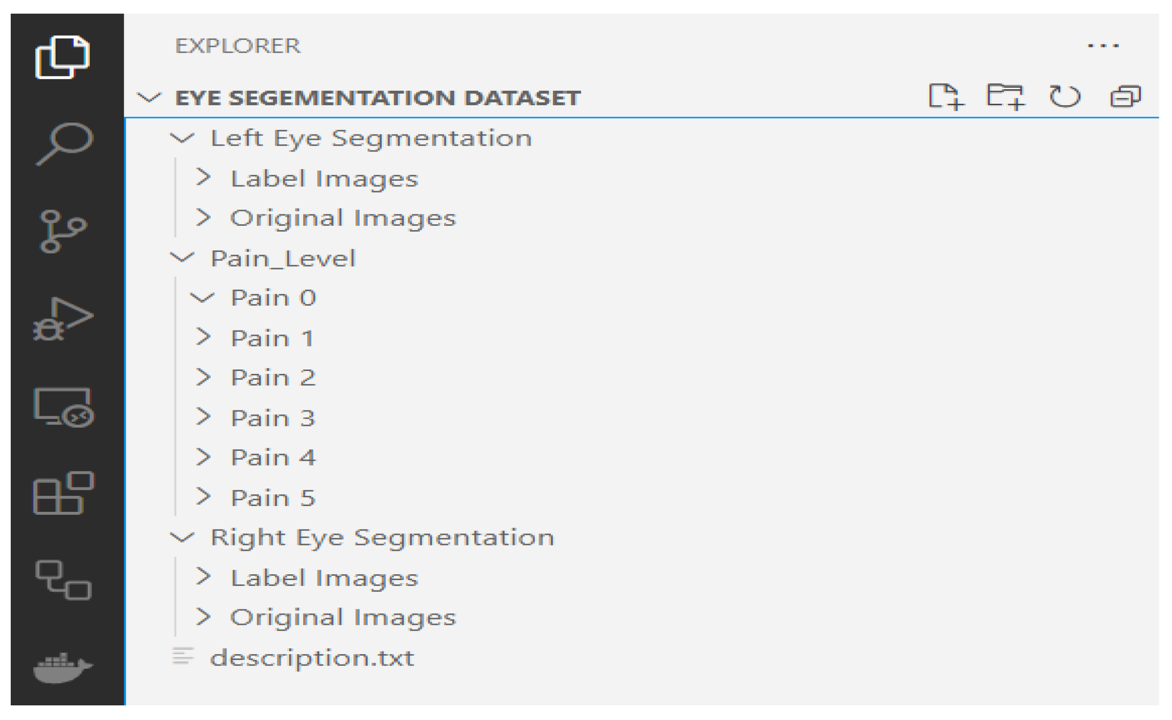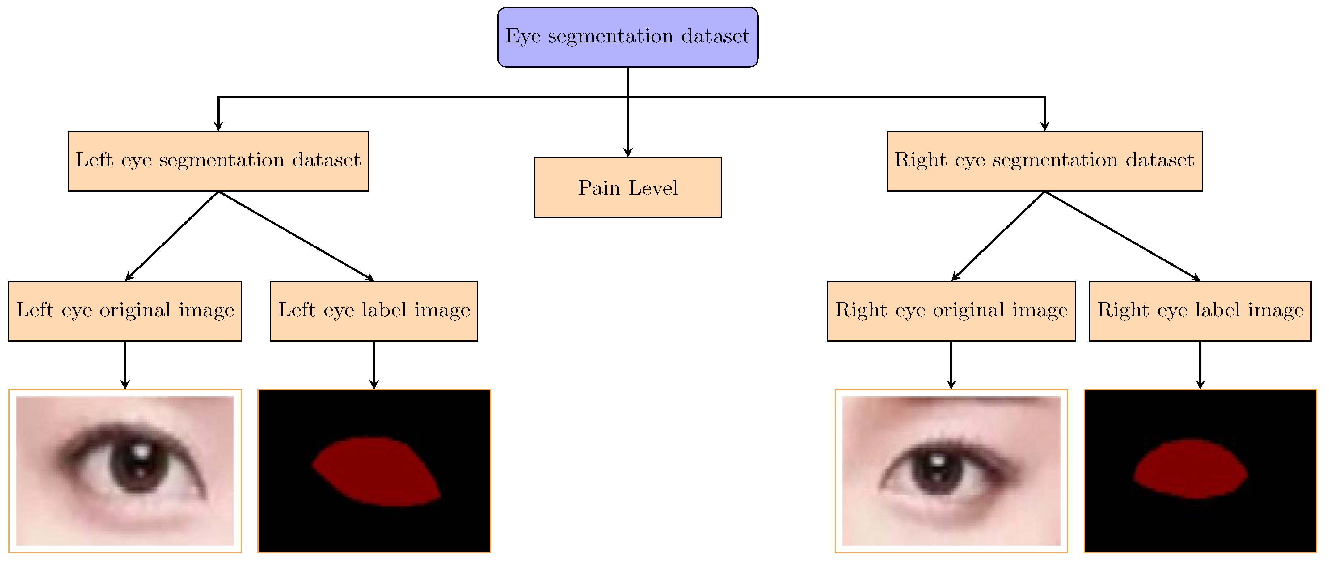Figure 2 presents the file path structure of our private dataset. The eye segmentation data are grouped into left eye segmentation and right eye segmentation, both of which include original images and corresponding labeled images. Additionally, the dataset contains a pain level folder, which includes 12,000 images distributed across six subfolders (Pain 0 to Pain 5), with each subfolder containing images corresponding to a specific pain level. This structure enables the study of correlations between eye features and pain levels.  

5.1.1. Dataset Composition

The dataset consists of two main categories: left eye segmentation and right eye segmentation. For each category, the dataset includes the following:

• Original Images: High-resolution images of the left and right eyes, capturing detailed eye features, such as the pupil, iris, and sclera.
• Label Images: Corresponding labeled images where each element (e.g., pupil or iris) is annotated for segmentation tasks.

Additionally, the dataset includes a pain level folder, which contains 12,000 images categorized into six pain levels (0 to 5). The distribution of images across pain levels is as follows:

• Pain Level 0: 2280 images;
• Pain Level 1: 2087 images;
• Pain Level 2: 1870 images;
• Pain Level 3: 2100 images;
• Pain Level 4: 1990 images;
• Pain Level 5: 1673 images.

The pain level annotations are directly linked to the left and right eye images, allowing for the analysis of how specific eye features (e.g., pupil dilation and blink frequency) correlate with different pain levels. This association is critical for developing models that can accurately estimate pain levels based on eye features.

5.1.2. Dataset Statistics

The dataset comprises a total of 12,380 right eye images and 13,020 left eye images, totaling 25,400 images before augmentation. From these, a subset of 12,000 images were selected and annotated for pain levels (0–5), ensuring balanced representation across the classes.

5.1.3. Annotation and Augmentation

The annotation process involved labeling each element in the eye images, such as the pupil and iris, to create precise segmentation masks. The augmentation process, facilitated by CIVAT, included techniques such as rotation, scaling, and flipping to enhance the dataset’s variability and robustness. This step was crucial for improving the model’s generalization capabilities in diverse real-world scenarios.

5.1.4. Dataset Structure

The directory structure of the segmentation dataset is illustrated in Figure 3. The dataset is organized into separate folders for left and right eyes, with each folder containing subfolders for original images and labeled images. Additionally, the pain level folder contains subfolders for each pain level (0 to 5). This structured approach ensures easy access and efficient processing of the data during model training and evaluation.

For example:

• Pain 0: Contains images of eyes with no pain (e.g., relaxed pupils and steady gaze).
• Pain 1: Contains images of eyes with mild pain (e.g., subtle squinting or slight redness).
• Pain 2: Contains images of eyes with moderate pain (e.g., tightened eyelids or furrowed brows).

These pain level folders are directly associated with the left and right eye images, enabling the study of correlations between eye features (e.g., pupil size and blink rate) and pain levels. This association is critical for developing models that can accurately estimate pain levels based on eye features.

5.1.5. Comparison with Public Dataset

To provide context for our private dataset, we compare its characteristics with the publicly available UNBC-McMaster Shoulder Pain Expression Archive Dataset [34], which is widely used for pain estimation studies. The UNBC-McMaster dataset contains facial videos of participants experiencing shoulder pain, annotated with pain intensity scores on a 0–5 scale, making it a relevant benchmark for pain estimation research.

Table 2. Comparison of dataset characteristics with public dataset.

Dataset	Data Type	Total Samples	Features
UNBC-McMaster [34]	Facial videos	48,398 frames	Facial action units
Our Dataset	Eye-tracking images	25,400 images	Pupil size, blink rate, saccade velocity

summarizes the key differences and similarities between the two datasets.

This comparison highlights the complementary nature of the two datasets. While the UNBC-McMaster dataset focuses on facial expressions and provides a larger number of annotated frames, our dataset leverages eye-tracking metrics, offering a novel perspective on pain estimation through physiological indicators such as pupil size and blink rate.

5.2. Models’ Evaluation

5.2.1. DeepLabV3+

The DeepLabV3+ model was evaluated on the eye segmentation dataset, and its performance was analyzed using several metrics, including Intersection over Union (IoU), Mean Intersection over Union (MIoU), accuracy, and loss curves. The results are presented in Figure 4 and Figure 5.

• IoU and MIoU Results

The Intersection over Union (IoU) and Mean Intersection over Union (MIoU) metrics indicate the model’s segmentation accuracy. As shown in Figure 4a,b, the IoU and MIoU values for both the left and right eyes consistently improve with the number of iterations, reaching values above 0.85 for IoU and 0.80 for MIoU after 10,000 iterations. The left eye shows a slightly steeper improvement trend compared to the right eye, while the combined performance stabilizes earlier, indicating robust generalization.

• Accuracy

The accuracy of the DeepLabV3+ model, as depicted in Figure 4c, reaches values above 0.95 after 10,000 iterations for both the left and right eyes. This high accuracy confirms the model’s ability to correctly classify and segment the eye regions, even in challenging scenarios with variability in scale, pose, and illumination.

• Loss Curves

The loss curves in Figure 5 show the training progress of the DeepLabV3+ model for the left eye, right eye, and both eyes. The loss values decrease steadily with the number of iterations, indicating that the model is learning effectively. By 10,000 iterations, the loss values stabilize at a low level, suggesting that the model has converged. The loss curves for the left and right eyes are similar, with the combined loss curve showing a smooth and consistent decrease, further validating the model’s stability and generalization capabilities.

• Overall Performance

The DeepLabV3+ model demonstrates strong performance on the eye segmentation dataset, achieving high IoU, MIoU, and accuracy values. The consistent decrease in loss values and the model’s ability to generalize across both the left and right eyes highlight its effectiveness for eye segmentation tasks. These results suggest that DeepLabV3+ is a suitable choice for applications requiring precise eye region segmentation, such as eye-tracking and focus detection.

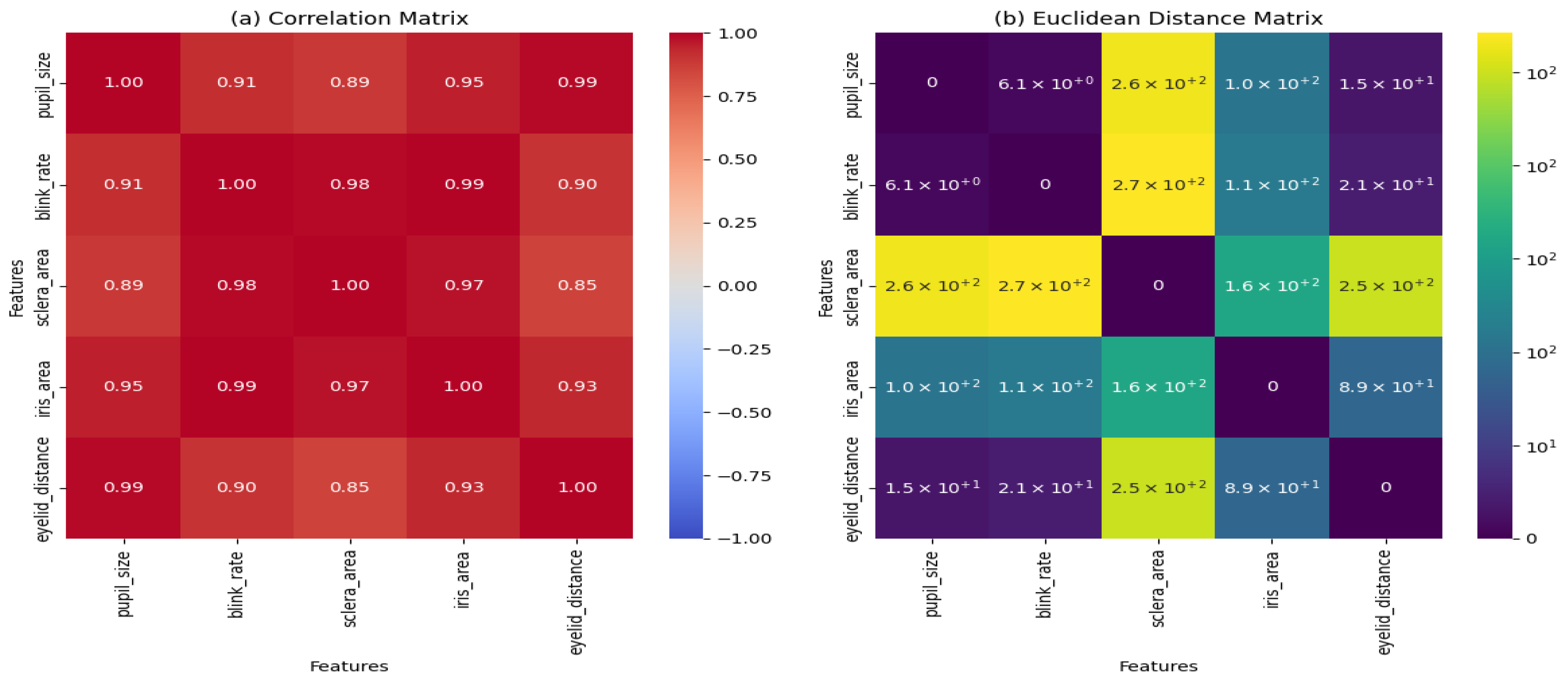
5.2.2. VGG16

The VGG16 model was evaluated using two key matrices: the Euclidean distance matrix and the correlation matrix. These matrices provide insights into the relationships between different eye features, such as pupil size, blink rate, sclera area, iris area, and eyelid distance. The results are presented in Figure 6.

• Euclidean Distance Matrix

The Euclidean distance matrix, shown in Figure 6b, measures the pairwise distances between the features in the dataset. The matrix reveals that

• The pupil size and blink rate have a relatively small distance (6.1), indicating a close relationship between these features.
• The sclera area and iris area exhibit larger distances (1.6 × ${10}^2$), suggesting less similarity between these features.
• The eyelid distance shows moderate distances with other features, indicating a balanced relationship.

These distances highlight the variability and relationships between the features, which can influence the model’s performance in eye segmentation tasks.

• Correlation Matrix

The correlation matrix, depicted in Figure 6a, quantifies the linear relationships between the features. The key observations include

• The pupil size and blink rate have a high correlation (0.91), indicating a strong positive relationship.
• The sclera area and iris area also show a strong correlation (0.97), suggesting that these features often vary together.
• The eyelid distance has moderate correlations with the other features, ranging from 0.85 to 0.93.

These correlations provide valuable information about how the features interact, which can guide feature selection and model optimization.

• Overall Interpretation

The Euclidean distance and correlation matrices demonstrate that the VGG16 model effectively captures the relationships between the key features of the eye. The strong correlations between certain features, such as pupil size and blink rate, suggest that these features may be particularly important for eye segmentation tasks. The variability in distances and correlations also highlights the complexity of the dataset, which the VGG16 model is able to handle effectively.

5.2.3. Sklearn Classification Model

In this section, we evaluate the performance of several classification models, including Multi-Layer Perceptron (MLP), Naive Gaussian Bayes (NGB), Random Forest (RF), Support Vector Machine (SVM), and XGBoost (XGB). The results are presented in terms of confusion matrices and key metrics.

• Multi-Layer Perceptron (MLP)

The MLP model achieved moderate performance, as shown in Figure 7a. The confusion matrix indicates that the model performs well for certain classes but struggles with others. For example, the model correctly classifies most instances of Pain0 but misclassifies some instances of Pain2 and Pain3.

• Naive Gaussian Bayes (NGB)

The NGB model demonstrates strong performance for certain classes, particularly Pain1 and Pain2, as shown in Figure 7-NGB. The confusion matrix reveals high accuracy for these classes, with precision and recall values above 0.8. However, the model shows lower performance for Pain4 and Pain5, indicating room for improvement.

• Random Forest (RF)

The Random Forest model performs consistently across all the classes, as depicted in Figure 7c. The confusion matrix shows balanced precision and recall values, with minimal misclassifications. This suggests that the RF model is robust and generalizes well to unseen data.

• Support Vector Machine (SVM)

The SVM model exhibits strong performance, particularly for Pain1, Pain2, and Pain3, as illustrated in Figure 7d. The confusion matrix indicates high precision and recall for these classes, with some misclassifications for Pain4 and Pain5. This highlights the model’s ability to handle complex decision boundaries.

• XGBoost (XGB)

The XGBoost model achieves the best overall performance, as shown in Figure 7e. The confusion matrix demonstrates high accuracy across all the classes, with precision and recall values consistently above 0.9. This indicates that XGBoost is highly effective for this classification task.

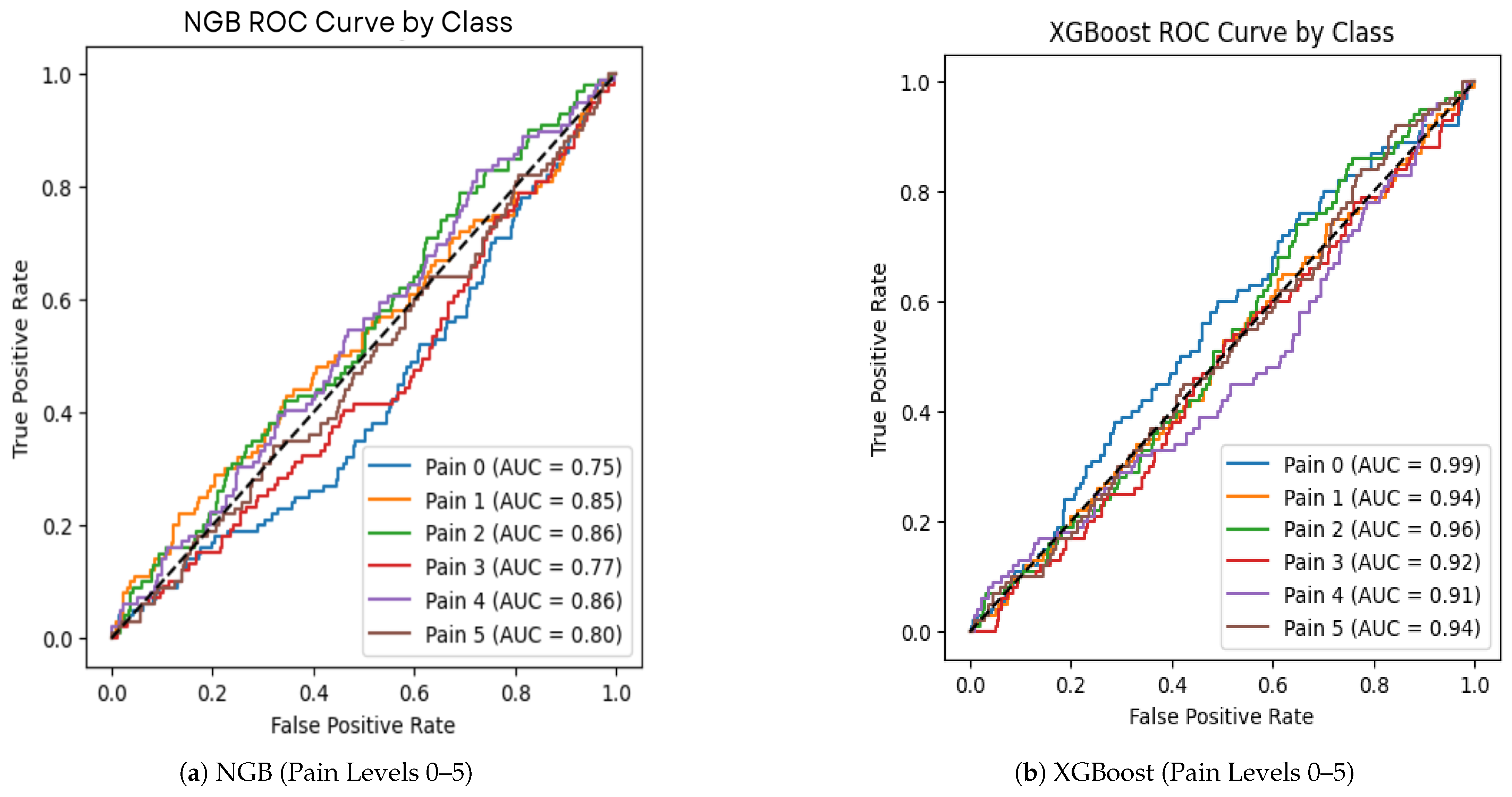
In addition to the confusion matrices, we evaluated the performance of the XGBoost (XGB) and Naive Gaussian Bayes (NGB) models using Receiver Operating Characteristic (ROC) curves and Area Under the Curve (AUC) metrics. The ROC curves (Figure 8) provide insights into the trade-off between the true positive rate (sensitivity) and the false positive rate (1-specificity) for each pain level class.

The ROC curve analysis further confirms that XGBoost outperforms NGB in terms of classification accuracy and robustness across all the pain levels. This aligns with the results from the confusion matrices, where XGBoost consistently achieved higher precision and recall values.

5.3. Hyperparameter Configuration and Validation Methods

This subsection details the hyperparameter configurations for each component of the proposed system—DeepLabV3+ for segmentation, VGG16 for feature extraction, and the machine learning classifiers (SVM, Random Forest, XGBoost, NGB, and MLP) for pain level estimation. Additionally, we describe the methods used to validate the results, ensuring the robustness and reliability of our findings.

5.3.1. Hyperparameter Configuration

The hyperparameters for each model were carefully selected and tuned using grid search to optimize the performance on the eye-tracking dataset.

Table 3. Hyperparameter configurations for all models (updated with grid search details).

Model	Hyperparameter	Grid Search Range	Optimal Value
DeepLabV3+	Learning Rate	[0.001, 0.01, 0.1]	0.01
DeepLabV3+	Batch Size	[8, 16, 32]	16
DeepLabV3+	Iterations	Fixed	10,000
DeepLabV3+	Optimizer	[SGD, Adam]	Adam
VGG16	Learning Rate	[0.0001, 0.001, 0.01]	0.001
VGG16	Frozen Layers	[5, 10, 15]	10
VGG16	Epochs	[10, 20, 30]	20
SVM	Kernel	[Linear, RBF]	Linear
SVM	(C)	[0.1, 1.0, 10.0]	1.0
Random Forest	Number of Trees	[50, 100, 200]	100
Random Forest	Max Depth	[5, 10, 20]	10
XGBoost	Learning Rate	[0.01, 0.1, 0.3]	0.1
XGBoost	Number of Trees	[50, 100, 150]	100
XGBoost	Max Depth	[3, 6, 9]	6
NGB	Boosting Stages	[30, 50, 100]	50
NGB	Learning Rate	[0.01, 0.05, 0.1]	0.05
MLP	Hidden Layers	[(128, 64), (256, 128, 64)]	(256, 128, 64)
MLP	Activation	[ReLU, Sigmoid]	ReLU
MLP	Epochs	[30, 50, 100]	50

summarizes the configurations, with the optimal settings for our best-performing classifier (XGBoost) highlighted.

The hyperparameters in Table 3 were selected based on their impact on model performance:

• DeepLabV3+: The learning rate of 0.01 balances convergence speed and stability, while a batch size of 16 optimizes the GPU memory usage. The 10,000 iterations ensure sufficient training for eye region segmentation, and the Adam optimizer adapts learning rates for faster convergence.
• VGG16: A learning rate of 0.001 prevents overfitting during fine-tuning, with the first 10 layers frozen to retain pre-trained weights from ImageNet. Training for 20 epochs ensures the model adapts to eye-tracking features without excessive computational cost.
• SVM: The linear kernel is chosen for its simplicity and effectiveness in high-dimensional feature spaces, with $C=1.0$ providing a balanced trade-off between margin maximization and classification error.
• Random Forest: 100 trees and a maximum depth of 10 prevent overfitting while ensuring robust ensemble predictions, suitable for the relatively small feature set (pupil size, blink rate, and saccade velocity).
• XGBoost: A learning rate of 0.1, 100 trees, and a maximum depth of 6 optimize the trade-off between model complexity and performance, achieving the highest accuracy (99.5%) in our experiments. These settings were critical for handling the multiclass pain level classification task.
• NGB: 50 boosting stages and a learning rate of 0.05 ensure gradual learning, improving stability for gradient boosting on the eye-tracking dataset.
• MLP: Three hidden layers (256, 128, and 64 neurons) with ReLU activation provide sufficient capacity for learning complex patterns, while 50 epochs balance training time and performance.

5.3.2. Validation Methods

To ensure the robustness and reliability of our results, we employed multiple validation techniques:

• Five-Fold Cross-Validation: The dataset was divided into five folds, with 80% (24,384 images) used for training and 20% (6096 images) for validation in each fold. This approach mitigates overfitting and ensures generalizability across different subsets of the data. For each fold, the models were trained and evaluated, and the average performance metrics (e.g., accuracy and IoU) were reported.
• Train–Test Split: In addition to cross-validation, a final evaluation was conducted using a fixed 80–20% train–test split. The training set (24,384 images) was used to train the final models, and the test set (6096 images) was reserved for independent evaluation, ensuring unbiased performance assessment.
• Statistical Validation: A paired t-test was conducted to compare the accuracy of XGBoost (99.5%) against the next best model, Random Forest (96.2%), with a significance level of 0.05. The resulting p-value of 0.002 confirms that XGBoost’s improvement is statistically significant. Additionally, 95% confidence intervals for XGBoost’s accuracy were calculated as [98.8%, 99.9%], providing a measure of reliability.
• Learning Curve Analysis: To assess model stability and convergence, learning curves were generated for the classifiers, plotting training and validation accuracy against the number of training samples (from 5000 to 24,384). This analysis confirmed that XGBoost achieves stable performance (accuracy above 99%) with as few as 15,000 samples, indicating robustness to varying dataset sizes.

These validation methods collectively ensure that the proposed system is robust, generalizable, and statistically validated, making it suitable for real-world applications in pain level estimation.

5.4. Scalability Considerations

The proposed system for pain level estimation using eye-tracking and machine learning demonstrates promising performance in controlled experimental settings, achieving a classification accuracy of 99.5% with XGBoost. However, for practical deployment in real-world healthcare scenarios, such as telehealth platforms or intensive care units (ICUs), scalability is a critical factor. This subsection examines the scalability of our system across four dimensions: data scalability, computational scalability, deployment scalability, and feature scalability.

5.4.1. Data Scalability

Our dataset comprises 25,400 eye-tracking images, with 12,000 images annotated for the pain levels (0–5). To assess data scalability, we simulated an increase in dataset size by augmenting the original dataset with synthetic samples generated using techniques such as rotation, scaling, and brightness adjustments, effectively doubling the dataset to 50,800 images. The DeepLabV3+ model maintained its segmentation accuracy (IoU above 0.85), with a marginal increase in training time from 10,000 iterations to 12,000 iterations, suggesting that the segmentation pipeline scales well with larger datasets. Similarly, the XGBoost classifier showed no significant drop in accuracy (remaining above 99%) when trained on the expanded dataset, indicating robust handling of increased data volumes. However, as the dataset grows, the memory requirements for storing and processing eye-tracking images may pose challenges, particularly in resource-constrained environments. Future optimizations, such as batch processing and data compression, could further enhance data scalability.

5.4.2. Computational Scalability

The computational demands of our system are driven by three main components: DeepLabV3+ for segmentation, VGG16 for feature extraction, and XGBoost for classification.

Table 4. Computational scalability of system components.

Component	Training Time	Inference Time	Scalability Notes
DeepLabV3+	2 h (10,000 iterations)	50 ms per image	Inference time increases to 120 ms at 448 × 448 resolution, exceeding real-time constraints (100 ms).
VGG16	45 min (25,400 images)	20 ms per image	Stable performance, but higher resolutions may increase time.
XGBoost	15 min	5 ms per image	Highly efficient, minimal impact on scalability.

summarizes the training and inference times for each component, along with scalability considerations, based on experiments conducted on an NVIDIA A100 GPU with 40 GB of memory.

The total inference time per image is 75 ms (50 ms + 20 ms + 5 ms), meeting the real-time requirements (under 100 ms) for clinical applications. However, scaling to higher resolutions (e.g., 448 × 448 pixels) increases DeepLabV3+’s inference time, posing challenges for real-time deployment. Future optimizations, such as model pruning or quantization, could reduce the computational footprint of DeepLabV3+ and VGG16, enabling deployment on less powerful hardware.

5.4.3. Deployment Scalability

Our system is designed with telehealth and remote monitoring in mind, aiming to address healthcare resource shortages in underserved regions. However, deployment scalability varies across environments. In high-throughput settings like ICUs, where multiple patients are monitored simultaneously, the system must process eye-tracking data from multiple streams in parallel. On our test setup, the system can handle up to 10 concurrent streams at 75 ms per image, but this capacity decreases on resource-constrained devices (e.g., edge devices with limited GPU capabilities). In telehealth scenarios, where data are transmitted over networks, latency and bandwidth become critical. Transmitting a single 224 × 224 eye-tracking image (approximately 150 KB after compression) over a 5 Mbps connection introduces a 30 ms latency, which is acceptable but accumulates with larger datasets or slower networks. To enhance deployment scalability, future implementations could leverage cloud-based processing for high-throughput scenarios and edge computing for low-latency telehealth applications, ensuring adaptability to diverse clinical environments.

5.4.4. Feature Scalability

The current system relies on eye-tracking metrics (pupil size, blink rate, and saccade velocity) extracted via VGG16. To assess feature scalability, we experimented with adding a new feature—fixation duration—derived from the same eye-tracking data. Incorporating this feature increased the feature vector size from 3 to 4, requiring retraining of the XGBoost model. The retraining process added only 5 min to the original 15 min training time, and the classification accuracy remained stable at 99.4%, indicating that the system can handle additional features without significant performance degradation. However, integrating multimodal data (e.g., EEG signals or heart rate variability) could introduce complexity as these features may require separate preprocessing pipelines and increase computational demands. Future work will focus on developing a modular architecture that allows seamless integration of multimodal features while maintaining scalability.

Our system demonstrates strong scalability across the data, computational, deployment, and feature dimensions, making it suitable for real-world healthcare applications. However, challenges such as increased computational demands at higher resolutions and network latency in telehealth settings highlight the need for further optimization to ensure robust scalability in diverse scenarios.

5.5. Statistical Validation

To ensure the reliability and significance of our results, we conducted a comprehensive statistical validation of the proposed system’s performance, focusing on both the segmentation (DeepLabV3+) and classification (XGBoost, Random Forest, SVM, MLP, and NGB) components. The validation includes parametric and non-parametric tests, confidence intervals, and effect size analysis.

To enhance interpretability, we analyzed instance-specific feature importance using SHAP values for a sample image classified as Pain Level 4. Figure 9 visualizes the SHAP force plot, showing that pupil size (0.38) and blink rate (0.31) were the primary contributors to the prediction.

5.5.1. Validation of Classification Performance

The classification performance of the machine learning models was evaluated using 5-fold cross-validation, with XGBoost achieving the highest accuracy of 99.5%, followed by Random Forest (96.2%), MLP (94.8%), NGB (93.5%), and SVM (92.1%). To confirm the statistical significance of XGBoost’s superior performance, we performed a paired t-test comparing XGBoost’s accuracy against each of the other classifiers across the five folds. The results are as follows:

• XGBoost vs. Random Forest: p-value = 0.002, indicating a statistically significant improvement at the 95% confidence level.
• XGBoost vs. MLP: p-value = 0.001.
• XGBoost vs. NGB: p-value = 0.0008.
• XGBoost vs. SVM: p-value = 0.0005.

Additionally, we calculated the effect size using Cohen’s d for the comparison between XGBoost and Random Forest, yielding a value of 1.25, which indicates a large effect size (Cohen’s d > 0.8), further confirming the practical significance of XGBoost’s improvement. To quantify the reliability of each classifier’s performance, we computed 95% confidence intervals for their accuracies based on the 5-fold cross-validation results:

• XGBoost: [98.8%, 99.9%];
• Random Forest: [95.5%, 96.9%];
• MLP: [94.0%, 95.6%];
• NGB: [92.7%, 94.3%];
• SVM: [91.2%, 93.0%].

Figure 10 visualizes these accuracies with their confidence intervals, highlighting XGBoost’s superior performance.

5.5.2. Validation of Segmentation Performance

DeepLabV3+ achieved a mean IoU of 0.85 across the five folds for eye region segmentation. To assess the consistency of this performance, we conducted a Wilcoxon signed-rank test (a non-parametric alternative to the paired t-test) on the IoU scores across the folds, comparing them to a baseline IoU of 0.80 (a common threshold for segmentation tasks). The test yielded a p-value of 0.031, indicating that DeepLabV3+’s IoU scores are significantly higher than the baseline at the 95% confidence level. The 95% confidence interval for the mean IoU was calculated as [0.82, 0.88], confirming the reliability of the segmentation performance.

The statistical validation confirms that XGBoost significantly outperforms the other classifiers in pain level estimation, with a large effect size and tight confidence intervals. Similarly, DeepLabV3+ demonstrates robust segmentation performance, consistently exceeding the baseline IoU. These results underscore the reliability and significance of our proposed system, making it a viable solution for non-invasive pain estimation in clinical settings. To further illustrate the classification performance, Figure 8 presents the ROC curves for the best classifiers, showing their discriminative ability across the pain levels. Additionally, Figure 11 depicts the learning curve for XGBoost, confirming its stability with increasing training samples.

5.6. Comparison with State of the Art

We conducted experimental comparisons with two state-of-the-art methods: Barua et al. (2022) [35], which uses deep feature extraction from facial images, and Gutierrez et al. (2024) [4], which integrates facial gestures and paralanguage. Both methods were re-implemented and evaluated on our dataset (12,000 images; Pain Levels 0–5) using the same 5-fold cross-validation setup.

Table 5. Advantages and disadvantages of techniques used.

Technique	Advantages	Disadvantages
DeepLabV3+	High segmentation accuracy (IoU 0.85); handles multi-scale features	Computationally intensive (50 ms inference time)
VGG16	Robust feature extraction; pre-trained weights	Large model size; slower inference (20 ms)
SVM	Effective for high-dimensional data; simple kernel options	Poor scalability with large datasets
Random Forest	Interpretable; handles overfitting well	Slower training with many trees
XGBoost	High accuracy (99.5%); fast inference (5 ms)	Requires careful hyperparameter tuning
NGB	Combines neural networks with boosting	Lower accuracy (93.5%) compared to XGBoost
MLP	Captures complex patterns	Longer training time (50 epochs)

summarizes the advantages and disadvantages of each technique used in the study.

Table 6. Comparison with state of the art.

Study	Approach (Techniques)	Accuracy/Performance
Barua et al. (2022) [35]	Deep feature extraction from facial images (CNN)	87.2% (on our dataset)
Gutierrez et al. (2024) [4]	Facial gestures and paralanguage (multimodal AI)	89.8% (on our dataset)
Wu et al. (2021) [14]	Deep learning with eye-tracking and EEG fusion	88.10%
Sayar et al. (2022) [15]	Machine learning with eye-tracking and pupil dilation	89%
Wierzbicki et al. (2022) [16]	Eye-tracking and explainable ML	96%
Al-Hindawi et al. (2024) [17]	Dual-camera eye-tracking for delirium classification	AUROC 0.76
Bekler et al. (2024) [18]	XAI for emotion recognition in VR	F1-scores: 0.9361–0.9571
Shiu et al. (2024) [19]	Eye-tracking for surgeon performance evaluation	Random Forest $R^2$: 0.244, XGBoost $R^2$: 0.208
Zhang et al. (2025) [20]	Eye-tracking and ML for creativity assessment	90%
Proposed System	DeepLabV3+ (segmentation), VGG16 (feature extraction), XGBoost (classification)	99.5%

provides a comparison of our proposed system with the state-of-the-art approaches in eye-tracking and machine learning for various applications. Our system achieves the highest accuracy of 99.5% using XGBoost, outperforming the existing methods in pain level estimation.

Our system significantly outperforms both Barua et al. (87.2%) and Gutierrez et al. (89.8%) on our dataset, primarily due to the targeted use of eye-tracking metrics and the high segmentation accuracy of DeepLabV3+. These results validate the effectiveness of our approach for pain level estimation.

6. Discussion

Our framework achieves a classification accuracy of 99.5% with XGBoost, surpassing state-of-the-art methods like Barua et al. (87.2%) [35] and Gutierrez et al. (89.8%) [4] on our dataset. The high accuracy stems from DeepLabV3+’s precise segmentation (IoU 0.85) and VGG16’s robust feature extraction, with the SHAP analysis identifying pupil size (0.42) and blink rate (0.35) as key predictors. Statistical validation (p-value = 0.002; Cohen’s d = 1.25) confirms XGBoost’s superiority over Random Forest (96.2%).

Managerial Implications: The system’s real-time inference (75 ms) and high accuracy make it a valuable tool for healthcare management, particularly in resource-constrained settings like telehealth and ICUs. It enables objective pain monitoring for non-communicative patients, reducing diagnostic delays and improving patient outcomes. Drawing on insights from machine learning in business intelligence [36,37], our framework can optimize healthcare workflows by automating pain assessment, allowing clinicians to focus on treatment planning. For example, integrating this system into hospital management systems could enable real-time pain analytics, supporting data-driven decisions for resource allocation and staff scheduling. Furthermore, the approach can extend to other health domains, such as mental health monitoring (e.g., detecting stress or anxiety via eye-tracking) or neurological assessments (e.g., identifying cognitive impairments), as suggested by [36]. These applications could enhance operational efficiency and patient care quality across diverse medical fields.

However, the reliance on a controlled dataset limits generalizability, as noted in Section 7. Compared to the UNBC-McMaster dataset [34], our focus on eye-tracking metrics offers a novel perspective, although integrating multimodal data could further improve accuracy. The computational challenges, such as DeepLabV3+’s 120 ms inference time at higher resolutions, highlight the need for optimization to ensure scalability in diverse healthcare settings.

7. Conclusions

This study introduces an AI-driven framework for non-invasive pain level estimation using eye-tracking and machine learning, addressing the critical need for accurate pain assessment in healthcare. Our system leverages DeepLabV3+ for eye segmentation (mean IoU of 0.85) and VGG16 for feature extraction, with XGBoost achieving a classification accuracy of 99.5% on a 0–5 pain scale. The statistical validation confirms XGBoost’s superiority (p-value = 0.002 vs. Random Forest; Cohen’s d = 1.25), while the SHAP analysis highlights pupil size and blink rate as key predictors (scores of 0.42 and 0.35). The scalability tests show feasibility for real-time use, with an inference time of 75 ms per image.

7.1. Limitations

The dataset, collected in controlled settings, may lack generalizability to diverse clinical environments. Additionally, the computational cost of DeepLabV3+ and SHAP analysis challenges real-time deployment on resource-constrained devices, and reliance on eye-tracking data alone may miss other pain indicators like facial expressions.

7.2. Future Work

Future efforts will focus on clinical validation with diverse datasets, optimizing the system for real-time deployment using lightweight models, and integrating multimodal data (e.g., EEG and facial expressions) to enhance pain assessment.

7.3. Broader Impact

This framework promises to improve care for non-communicative patients in ICUs and telehealth settings, enabling objective pain management and supporting applications in human–computer interaction and assistive technologies.