Lossless Compression of Malaria-Infected Erythrocyte Images Using Vision Transformer and Deep Autoencoders

Abstract

Lossless compression of medical images allows for rapid image data exchange and faithful recovery of the compressed data for medical image assessment. There are many useful telemedicine applications, for example in diagnosing conditions such as malaria in resource-limited regions. This paper presents a novel machine learning-based approach where lossless compression of malaria-infected erythrocyte images is assisted by cutting-edge classifiers. To this end, we first use a Vision Transformer to classify images into two categories: those cells that are infected with malaria and those that are not. We then employ distinct deep autoencoders for each category, which not only reduces the dimensions of the image data but also preserves crucial diagnostic information. To ensure no loss in reconstructed image quality, we further compress the residuals produced by these autoencoders using the Huffman code. Simulation results show that the proposed method achieves lower overall bit rates and thus higher compression ratios than traditional compression schemes such as JPEG 2000, JPEG-LS, and CALIC. This strategy holds significant potential for effective telemedicine applications and can improve diagnostic capabilities in regions impacted by malaria.

1. Introduction

Malaria continues to be a serious worldwide health concern that causes a great deal of illness and death across the globe, particularly in areas with limited resources [1]. Through the bites of female Anopheles mosquitoes carrying Plasmodium parasites, humans can contract this life-threatening disease [2]. In line with the World Health Organization (WHO)’s findings, the global malaria incidence was expected to be 263 million cases in 2023, or 60.4 cases per 1000 at-risk individuals. A total of 597,000 fatalities were estimated, resulting in a mortality rate of 13.7 per 100,000 population [3]. If diagnosed early, malaria is a preventable and curable illness [4]. Traditional diagnostic methods, including inspection of Giemsa-stained blood samples under an electron microscope, take a lot of time, are prone to mistakes, and require a high degree of skill that may not be available in remote areas [5]. Moreover, the urgent requirement for accurate diagnoses and the inherent heterogeneity in sample quality underscore the need for advancements in diagnostic methodologies [6].

Effective computer-assisted systems for malaria infection study and the Internet allow biomedical images to be shared globally. Experts situated in different parts of the world can now work together and assess cases. Light microscopic images and whole-slide images are the two main image types used in computer-assisted malaria diagnosis [7]. Whole-slide images have become increasingly popular due to recent increases in processing power, cloud computing, and sophisticated algorithms. Several studies previously concentrated on light microscopic pictures [8,9,10,11,12], which typically have a poorer resolution. High-resolution images offer a more comprehensive depiction of medical conditions, enabling ML algorithms to identify subtle patterns and irregularities that may go unnoticed in lower-resolution images. This enhanced detail is vital for accurate diagnostic evaluations but poses challenges due to higher bandwidth and storage demands [13]. To address this challenge, it is crucial to employ sophisticated lossless compression methods that will maintain the diagnostic integrity of the images while decreasing the file sizes for more efficient transmission and storage. In the following, we first provide a brief overview of the current advances in the automated diagnosis of malaria infection using machine-learning algorithms. Since the aim of our paper is on efficient lossless compression, we then surveyed studies that addressed the relation between image data compression and image pattern classification.

ResNet34 [14], a type of neural network (deep convolutional), was used in [15] to analyze cell images for the detection of malaria, attaining impressive accuracy rates. This study relied on a collection of images of both infected and uninfected erythrocyte cells, showcasing the network’s capability to reliably determine infection status, which could greatly support early diagnosis and treatment approaches for malaria. In this paper [16], the author presents a Convolutional Neural Network (CNN) model designed to classify images of malaria-infected cells, achieving impressive accuracy along with strong feature extraction capabilities. The proposed model effectively identifies infected cells, enabling the calculation of parasitemia and demonstrating considerable improvement over earlier diagnostic techniques. Yebasse et al. [17] developed a strategy to improve malaria detection by emphasizing infected areas in cell images, resulting in higher classification precision across various models, including Resnet [18] and Mobilenet [19]. A hybrid system for classifying images of malaria utilizes a CNN model for extracting features along with a KNN algorithm (K-nearest neighbor) [20]. This method accurately distinguishes between distinct stages of Plasmodium Vivax and Plasmodium Falciparum, indicating the possibility of increasing the accuracy and effectiveness of malaria diagnosis. Liang et al. [21] addressed a sophisticated 16-layer CNN model for diagnosing malaria that accurately categorizes red blood cells in blood smears as infected or non-infected. This approach outperforms traditional methods by providing a reliable, automated diagnostic solution that could significantly enhance malaria screening and monitoring. Saravan et al. [22] improved the quality of malaria cell images by implementing preprocessing techniques, including normalization and data augmentation methods such as rotation and flipping. They also utilized deep-learning models for feature extraction to effectively classify cells as either infected or non-infected, thus greatly enhancing the diagnostic process. A CNN model that improves malaria detection by evaluating a specific pile of blood stain images captured with a specially designed image scanner was addressed in [23]. This model enhances both the sensitivity and specificity when identifying Plasmodium falciparum infections. The author in [24] presents a hybrid deep learning architecture that combines VGG19 [25] and SVM [26] for malaria diagnosis in microscopic pictures. Their strategy uses transfer learning to boost VGG19’s feature extraction capability while using SVM’s classification power, resulting in an impressive $95\%$ classification accuracy. The proposed model offers a considerable increase in the automated identification of malaria, outperforming standard CNN models. In summary, there have been substantial studies in the literature on deep-learning methods for image classification for the diagnosis of malaria infection.

It turns out that there is an interesting interplay between data compression and data pattern classification. In [27], the authors challenged the widely held belief that JPEG compression has a negative impact on deep-learning performance, by demonstrating that selecting the appropriate compression levels can actually improve classification accuracy while decreasing data size. This work demonstrated the advantage of combining the tasks of image compression with classification. In this paper [28], the author studied how image compression impacts deep-learning models used to identify mammograms, and argued that moderate compression levels preserve classification accuracy. This study shows the feasibility of applying image compression in clinical contexts to optimize storage while maintaining diagnostic efficacy. In [29], the authors investigated how JPEG, JPEG2000, and HEVC compression influence CNN image classification, showing that considerable compression can occur with minimal impact on accuracy. They showed how to determine the optimal compression settings to maintain neural network effectiveness. In this paper [30], the author reported the unexpected influence of JPEG and SVD compression on image classification accuracy using the Inception-v3 model. The paper showed that using moderate-to-high levels of compression frequently improved classification performance across a diverse collection of images, implying that compression could be a useful preprocessing strategy in CNN applications. This observation reveals potential real-world applications for improving image classification’s effectiveness and accuracy. The author in [31] developed a quantum machine-learning framework capable of classifying larger images with fewer qubits than previous techniques, attaining comparable accuracy to classical neural networks. The encoding approach and quantum neural network design represent a step forward in quantum machine learning’s practical applications. In this work [32], the author addressed Wavelet-based transform for classification using an SVM (Support Vector Machine) in which wavelet transformation and run-length encoding were utilized for efficient compression. A method for lossless image compression that utilizes prediction errors, employing an artificial neural network (ANN) for the prediction phase and Huffman coding for entropy encoding, was discussed in [33]. On a variety of datasets, it was shown that applying a fuzzy c-means algorithm together with wavelet transformation and Fourier classification features improved compression efficiency.

Based on the background research, we observe that the existing work is fairly sparse on using pattern classification to assist in data compression, especially for lossless data compression. To this end, we propose to introduce the state-of-the-art Vision Transformer (ViT) as a high-performance classifier for malaria-infected cell images by capitalizing on ViT’s self-attention mechanism, which allows this model to efficiently learn the inherent connections among the image pixel values. More specifically, we first classify the input images into different categories and then pass the classified images to separate deep autoencoders that perform data reduction. This procedure allows the autoencoders to exploit common patterns from the images in the same category, as each autoencoder is trained on images of the same class. By concentrating on these shared traits, the autoencoders are expected to better capture particular features than would be possible if we do not separate the input images into different categories, thereby improving the overall compression efficiencies on the entire dataset.

The remainder of this paper is organized as follows: the source of the dataset is presented in Section 2; the underlying theories and methods used in this study are presented in Section 3; the research findings are presented in Section 4; the study’s limitations and possible directions for future research are discussed in Section 5; and we drew conclusions in Section 6.

2. Malaria Dataset

2.1. UAB Dataset

In our work, we utilized digital whole-slide images from the PEIR-VM database, which is maintained by the University of Alabama at Birmingham (UAB) [34]. The images were recorded as uncompressed TIFF files and converted to JPEG format to save storage space. They were then scanned digitally using a 40× objective using the Aperio™ Whole Slide Image Scanner (manufactured by Leica Biosystems in Nussloch, Germany). Image processing methods such as segmentation and denoising were employed to create clear images of individual cells. The MediaWiki platform was used to reorganize the image libraries, and Wright–Giemsa staining was applied to improve the visibility of essential cellular components, assisting in the detailed examination and labeling performed that was achieved by UAB pathologists. The final dataset consisted of 2565 cell images, divided into 1034 infected and 1531 uninfected samples [35].

2.2. NIH Dataset

The Malaria Screener dataset, compiled from thin blood smears stained with Giemsa, includes a significant number of 27,558 cell images. These images were collected from 193 patients—148 who were infected with Plasmodium falciparum and 45 who were non-infected—at Chittagong Medical College Hospital in Bangladesh and available on the National Institutes of Health website [36]. The complete dataset was evenly split between cells that were infected (parasitized) and those that were uninfected. In total, there were 13,779 images of infected cells and an equal number of images of uninfected cells. Each image in the collection is labeled with details that include not only the parasite status but also the identification of air bubbles, debris, and white blood cells—all of which are frequently discovered during blood sample analyses.

3. Materials and Methods

3.1. Deep Learning for Image Classification and Compression

Deep learning makes use of multi-layered artificial neural networks (ANNs) to identify complex patterns in data through non-linear transformations. Due to its ability to autonomously recognize and improve the features from raw data, deep learning performs very well in applications including image identification, speech recognition, fraud detection, medical diagnostics [37], and video data analysis, particularly for counting repetitive actions [38]. In contrast to traditional approaches, deep learning drastically decreases the need for human feature extraction, resulting in excellent scalability for extensive datasets. Its inherent independence enables applications across multiple learning techniques, including supervised, semi-supervised, and unsupervised learning [39].

3.2. Image Classification

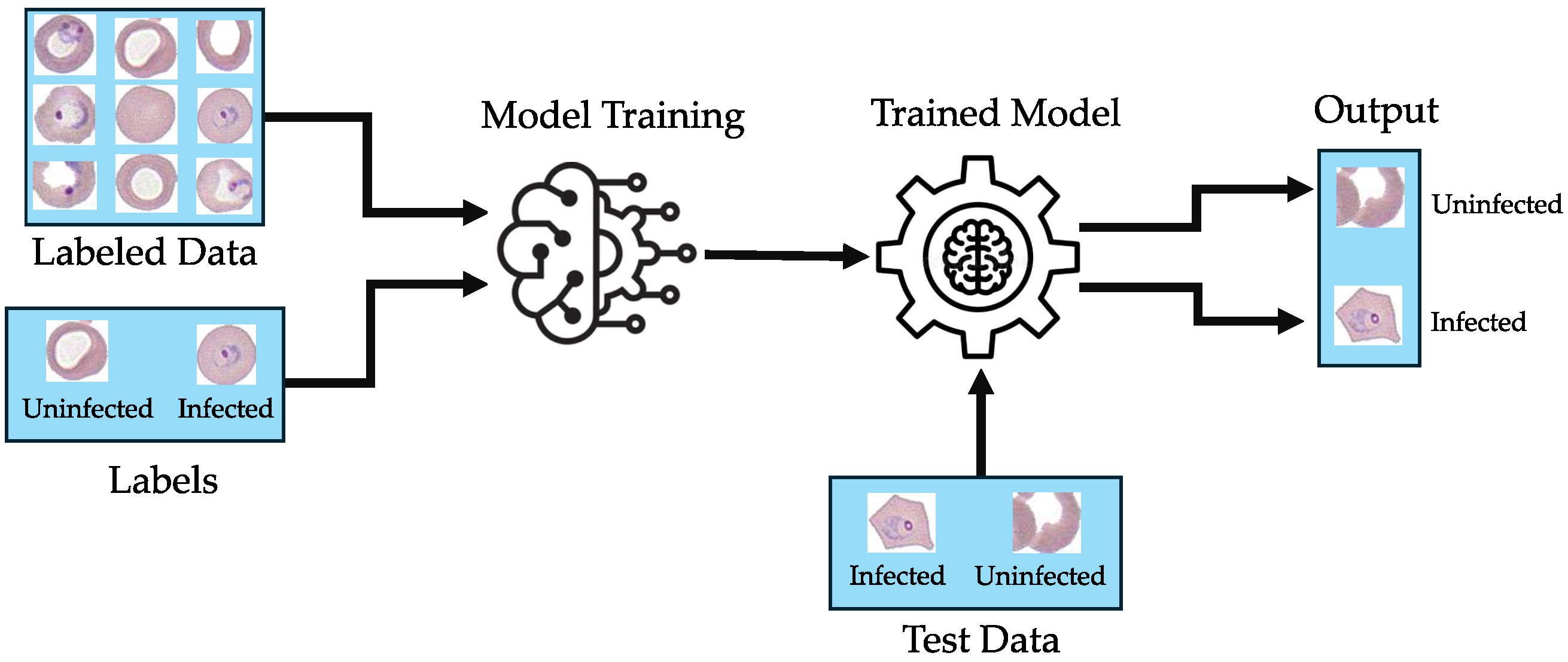
Image classification is a crucial task in visual computing that involves categorizing images into certain classes, as determined by the image content. The whole process mainly employs supervised learning methodologies, where the model is trained on a dataset that has been explicitly labeled to connect specific image features with their respective class labels [40]. This strategy is analogous to teaching an individual how to identify different objects by highlighting their unique features. In supervised learning, various deep-learning models such as Dense Convolutional Networks (DenseNets) [41], deep autoencoders [42], Convolutional Neural Networks (CNNs) [43], Vision Transformers (ViTs) [44], etc., are used in image classification or prediction to extract important features. Figure 1 shows the general framework for malaria-infected red blood cell image classification.

3.3. Vision Transformers

Vision Transformers (ViTs), a deep-learning model that demonstrates an architectural advancement in computer vision, are primarily created for natural language processing. ViTs use the full potential of self-attention mechanisms for image processing [44]. ViTs are widely used in common image identification tasks such as object detection, motion recognition, and image classification. In ViTs, an image is first divided into uniform patches, which are subsequently flattened and precisely transformed into embeddings. Positional embeddings are added to offer spatial context, which is important because transformers cannot process data in sequence. The sequence is then fed to the transformer encoder as an input. Additionally, the sequence includes a “classification token” that is learnable for aggregating features across the image to aid in classification [45]. The Vision Transformer (ViT) encoder is composed of several blocks, each of which has three key elements: Multi-Layer Perceptrons (MLPs), a Multi-head Attention Mechanism, and Layer Normalization. The architecture of the ViT is depicted in Figure 2, with a detailed explanation of the key elements given below:

• Layer Normalization allows the model to adjust to the differences between the training images and ensures that the training process remains steady.
• Using the provided embedded categorization tokens, the Multi-head Attention Network generates attention maps. The network can concentrate on the most important areas of the image, such as objects, thanks to these attention maps.
• The MLP is a two-layer classification neural network that terminates with a Gaussian Error Linear Unit (GELU). The last segment of the MLP, known as the MLP head, functions as the transformer’s output. By utilizing softmax on this output, it is possible to produce classification labels (for example, in the scenario of image classification).

3.4. Autoencoder

Autoencoders (AEs) are a type of artificial neural network (ANN) designed for unsupervised learning to achieve dimensionality reduction and feature extraction [39]. AE models function by reducing the input data into a latent-space description before attempting to reconstruct the input data so as to reduce the loss between the original input and its reconstructed version [46]. Figure 3 illustrates the architecture of an autoencoder.

Autoencoders (AEs) are in general feed-forward networks, typically consisting of three layers (input, output, and hidden layers). Several variants of AEs have been studied in the literature. Each variant serves a different purpose, starting with basic input data reduction to complex input data modeling.

• Convolutional Autoencoders (CAEs) are specifically designed for image data and use convolutional layers to efficiently record spatial hierarchies [47].
• Denoising Autoencoders are used when where the model’s input differs from its output. For instance, the model might receive low-quality corrupted images as input and then enhance the image quality in its output [46].
• Sparse Autoencoders implement sparsity in the hidden layers in order to gain more unique features.
• Variational Autoencoders (VAEs), characterized by their generative capabilities, possess the ability to generate new data points derived from the established distribution [39].
• Stacked Autoencoders (SAEs), which are made up of multiple layers of autoencoders, are particularly effective at capturing hierarchical representations, making them suitable for complex tasks in image and speech recognition [48].
• Deep Autoencoders (DAEs) are a type of neural network featuring an encoder and decoder design that condense data into a latent space and reconstruct them. These decoders detect complex patterns that are beneficial for activities like dimensionality reduction, denoising, and anomaly detection by minimizing reconstruction loss.

3.5. Huffman Encoding

Huffman coding is an algorithm for lossless data compression based on entropy encoding. This algorithm aims to minimize coding redundancy while maintaining data quality [49,50]. The core idea of the Huffman encoding algorithm is to make use of the frequency of the data. The method used in the algorithm allocates symbols from the alphabet with varying code lengths based on their occurrence rates [51]. Symbols that are used more frequently are represented by shorter codes to achieve better compression results [52]. Here, the symbols with the lowest probabilities are combined, and this procedure continues until only two probabilities of combined symbols remain, resulting in the formation of a code tree from which Huffman codes are derived through the labeling of this tree. Figure 4 demonstrates the Huffman algorithm through an example.

The overall procedure for generating a Huffman tree can be illustrated in five steps.

Step 1: List the symbols from highest to lowest probability order (Stage-I in the Huffman tree).

Step 2: The lowest two probabilities are combined to obtain a new composite symbol. Then, again check for the highest to lowest order of probabilities. If required, sort the symbols (including the composite symbols) (Stage-II in the Huffman code tree).

Step 3: Repeat Step 2 until there are only two symbols left (with the sum of their probabilities being equal to 1) (Stage-V in the Huffman code tree).

Step 4: Assign 0 and 1 to each stage of the Huffman tree. Throughout each stage, the top and bottom probabilities will be assigned as 0 and 1, respectively. Search forward from the last stage to the first stage, the Huffman code for each symbol is the set of all 0’s and 1’s on that path.

Step 5: The lengths of the Huffman codes given to each symbol $(S_0,S_1,\cdots ,S_n)$ and their corresponding probabilities define the average length of code in Huffman coding. Refer to the following equation to determine the ACL.

$$ACL=\sum _{k=1}^{n}Prob\left(k\right)·\mathrm{length}\left(S_k\right)$$

(1)

In this equation, ACL stands for the Average Code Length of the Huffman coding algorithm and $\mathrm{length}\left(S_k\right)$ is the collection of all the 0’s and 1’s in $S_k$.

The probability sequence in the aforementioned example has an average code length (ACL) of 2.38.

$$\begin{array}{l}ACL=0.30\times 2+0.25\times 2+0.20\times 2+0.12\times 3+0.08\times 4+0.05\times 4\\ \hspace{1em} =2.38\end{array}$$

3.6. Lossless Image Compression Techniques

Digital images often contain a significant amount of redundancy, the elimination of which can lead to significant data compression, which in turn can reduce storage requirements as well as transmission bandwidth. Lossless image compression is a reversible process with exact reconstruction of the original image [53,54]. Lossless image compression is primarily used in situations where maintaining the original quality of the image is crucial, including in fields such as medical imaging, scientific data visualization, technical illustrations and schematics, remote sensing tasks, and military communications [55]. Advanced lossless image compression methods include run-length coding, Huffman coding, arithmetic coding, JPEG 2000, JPEG-LS, CALIC, etc. [56]. Moreover, these methods utilize sophisticated algorithms that can exploit unique features of the image data, resulting in higher compression ratios while ensuring there is no loss of image quality. Recent advancements have focused on refining these algorithms with machine-learning models that anticipate coding patterns based on the image’s context [57].

3.6.1. JPEG 2000

JPEG 2000 represents a notable improvement over the conventional JPEG format, providing a more flexible and efficient method for image compression that accommodates both lossless and lossy techniques [58]. The versatility of JPEG 2000 makes it appropriate for a variety of applications, including digital cinematography and archiving, where image quality and integrity are crucial. JPEG 2000 relies on discrete wavelet transforms (DWTs) as opposed to JPEG’s dependence on discrete cosine transforms (DCTs) [54]. Wavelets excel in compressing images with a high resolution, yielding higher compression ratios and quality. A pyramidal structure can be formed using the wavelet decomposition technique based on sub-bands, which captures image details across various resolutions, including the resolution of the original image. An important drawback to keep in mind is that JPEG 2000 faces limited compatibility with the majority of browsers due to the complexities involved in its encoding and decoding procedures [59].

3.6.2. JPEG-LS

JPEG-LS, which stands for the Joint Photographic Experts Group Lossless Standard, is a sophisticated image compression standard that balances simplicity, efficiency, and performance [60]. Designed especially for circumstances when lossless or near-lossless compression is crucial, like in medical imaging and professional photography, JPEG-LS is based on the LOw COmplexity LOssless COmpression for Images (LOCO-I) algorithm developed by Hewlett-Packard [61]. JPEG-LS achieves high performance by employing a predictive coding approach that estimates the current pixel value from its adjacent pixels. Following this estimation, the prediction errors are calculated and encoded using Golomb–Rice coding, which is particularly useful for data having a geometric distribution. This method enhances the efficiency of JPEG-LS by greatly minimizing data size while preserving complete fidelity, guaranteeing that no original image data are lost during the compression and decompression process [62]. Additionally, JPEG-LS accommodates various image formats, such as continuous-tone and bi-level images, highlighting its adaptability.

3.6.3. CALIC

The Context-based Adaptive Lossless Image Codec (CALIC) is an important milestone in the field of lossless image compression [56]. CALIC is designed to preserve the original image’s integrity while greatly increasing compression efficiency. It employs an advanced prediction model that adjusts gradients dynamically according to the local image gradients [63]. The model enables accurate prediction of pixel values, which considerably minimizes redundancy and subsequently decreases the size of the compressed image file [64]. CALIC’s advanced algorithms surpass conventional lossless techniques by incorporating a wide array of modeling contexts, which improves the ability to accurately customize its predictive method according to various image statistics, leading to superior compression ratios compared to earlier formats like JPEG-LS or PNG, especially for images with complex textures or significant detail [65]. In addition, CALIC has been modified and improved in several applications to feature functionalities such as simultaneous encryption and compression of images, demonstrating its adaptability and strength in maintaining security along with compression [64].

3.7. Vision Transformer for Image Classification

The ViT model is a neural network that employs the transformer architecture to encode the input images into feature vectors. This network comprises two primary elements: the backbone, which converts images into a vector of features, and the head, which analyzes these vectors to generate prediction scores.

In this work, we need to classify our dataset before compression. To do this, we employed a pre-trained Vision Transformer (ViT) network to classify our dataset effectively. Due to ViT’s pre-learned features, we did not have to train the model from scratch for our own dataset. We modified the classification head and made necessary changes to the settings required for our datasets.

The pre-trained model was loaded using the “visionTransformer” function from MATLAB’s (R2024a) Computer Vision Toolbox, which provides a base-sized ViT neural architecture [66] featuring a patch dimension of 16. This network was fine-tuned utilizing the ImageNet 2012 dataset at a resolution of 384 by 384 pixels [67]. So the images in our dataset were resized to match this input resolution requirement. In the pre-processing phase, we created an image datastore to store the resized images. We fine-tuned the attention layers while keeping the other trainable parameters frozen. After that, the stored data were divided into three sets: training, validation, and testing. To enhance the training process, the “imageDataAugmenter” function was utilized, incorporating random reflection, rotation, scaling, and horizontal flipping. Subsequently, we generated augmented image datastores that adjust the dimensions of the validation and testing images to align with the input size required by the network. We adjusted the model to produce predictions that were particular to the classes in our dataset by changing the classification head. This modification is illustrated in Figure 5.

After adjusting the new classification head, we establish a new fully connected layer with an output dimension that corresponds to the number of classes in our training dataset. Next, we substitute the existing fully connected layer with the newly created one. Subsequently, our data are ready for training. Thus, we need to define the training parameters, including selecting the Adam optimizer, setting the learning rate to 0.0001, training for 30 epochs, using a mini-batch size of 6, and designating the GPU as the execution environment, among other settings. We opted for the Adam optimizer because it is highly valued and can dynamically modify the learning rates for individual parameters, enabling more efficient optimization of deep learning models compared to traditional methods such as Stochastic Gradient Descent (SGD) [68,69]. Moreover, we chose a smaller mini-batch size because using larger mini-batches during training caused us to run out of memory. Training a Vision Transformer (ViT) model typically requires considerable memory resources [70]. As a solution, one option is to employ a smaller variant, like a tiny-sized ViT model, or to decrease the mini-batch size [71,72]. Also, using a lower learning rate (0.0005) helps to adjust the transformer’s weights while preserving the essential feature recognition of the pre-trained model.

We used the “trainnet” function to train our neural network. Cross-entropy loss is utilized for classification purposes. A primary benefit of utilizing cross-entropy loss, particularly in classification tasks, is that it provides a comprehensive assessment of the difference between the probability distribution predicted by the model and the actual distribution of the labels [73]. By default, the trainnet function uses a GPU if it is accessible, although we have the option to define the execution environment. To train on a GPU, a Parallel Computing Toolbox and a supported GPU device are necessary. If a GPU is not available, the trainnet function will use the CPU instead. The accuracy of the trained data, test data, and validation data is calculated using the following equation.

$$\mathit{Accuracy}={\displaystyle \frac{TrPos+TrNeg}{TrPos+FlPos+TrNeg+FlNeg}}$$

(2)

where the variables can be defined as follows:

• True Positive ($TrPos$) refers to the correct identification of infected images.
• True Negative ($TrNeg$) refers to the correct identification of non-infected images.
• False Positive ($FlPos$) refers to the incorrect identification of infected images.
• False Negative ($FlNeg$) refers to the incorrect identification of non-infected images.

Accuracy is defined as the proportion of accurately predicted cases to all cases. This measure is used to assess the overall correctness of the model [74].

3.8. The Proposed Lossless Image Compression Method

We trained a deep autoencoder for input image size reduction. The decoder part of the autoencoder reconstructs the input image. The deep autoencoder introduces some loss, as the image generated by the decoder is not exactly the same as the input image. We determine how much the input and reconstructed images differ (in terms of the residue) in order to make the procedure lossless, then compress the residue with Huffman encoding. The encoded residue vector and the latent representation from the encoder are combined to yield the final compact representation of the input, which can be used to reconstruct the original input image losslessly. Therefore, the proposed lossless compression scheme consists of two main components: deep autoencoder, followed by residue encoder. Figure 6 shows the architecture of the proposed lossless compression scheme.

The detailed architecture of the encoder part of the deep autoencoder is illustrated in Figure 7. A number of convolution and dense layers make up the model, which is designed to effectively reduce the dimensionality of the input image data. The encoder begins with two convolutional layers with kernel sizes of 32 and 64, respectively. To enhance the non-linear learning and stabilize the training procedure, each convolutional layer incorporates Batch Normalization and employs LeakyRelu activations. After each convolution step, the Max-pooling operation is performed with a stride of $2\times 2$ to generate low-dimension feature maps. The pooling operation is essential to strategically extract important features and to reduce the computational cost in subsequent layers, where two fully connected dense layers containing hidden units of 1000 and 500, respectively, are added to the encoder. The dense layers are activated by the Relu activation functions to facilitate non-linear learning without negatively impacting the gradient flow. The encoder concludes with a bottleneck layer consisting of 30 neurons. This compact representation is crucial for an effective reconstruction of the original data during the decoder phase.

The configuration of the decoder part of the deep autoencoder is presented in Figure 8, which performs the reverse operations of the encoder using symmetrical parameters to reconstruct the input image from the compact representation. Initially, the encoded representation is expanded via a series of dense layers. Subsequently, the resulting higher-dimensional data are reshaped into feature maps to be processed by the following deconvolution layers. The feature maps’ spatial dimensions are gradually doubled by the upsampling layers, which also restore the original image’s dimensions. A convolutional layer with a single filter creates the final output by scaling the pixel values between 0 and 1 using the sigmoid activation function. The cropping2D resolves any differences in dimensions that arise from the upsampling process.

To reduce the reconstruction error, the model incorporates the Adam optimizer and the mean square error loss function. The deep autoencoder is trained over 200 epochs for a batch size of 32. The proposed deep autoencoder model efficiently reduces the dimensionality of the input image by capturing the critical features of the input in a lower dimensional latent space. Simultaneously, the decoder retrieves the original image from the compressed format with minimal reconstruction error.

4. Results

4.1. Classification Performance Analysis of Vision Transformer on the UAB Dataset

To evaluate the Vision Transformer’s (ViT) classification ability, we implemented the model using MATLAB R2024a-64 bit on a system with the following specifications: Intel Core(TM) i7-5930K CPU operating at 3.50 GHz, with 64 GB of RAM, and an NVIDIA GeForce GTX TITAN X Graphics Processing Unit (GPU) that includes 12 GB memory and Ubuntu 22 OS. The erythrocyte image dataset contains a total of 2565 images for both classes (malaria-infected and non-infected or uninfected cells). The dataset was divided into three groups: $90\%$ for training, $5\%$ for validation, and $5\%$ for testing. While training, the batch size was selected as 6, epochs were set to 20, and the learning rate was chosen as 0.0005, which was found to offer the best performance in this work.

The resulting confusion chart, shown in Figure 9, demonstrates how well the Vision Transformer performs for image classification. Figure 9a displays the model’s prediction accuracy, concentrating solely on the training images. The infected cells are denoted as class 1, while the non-infected cells are classified as class 0. This chart also indicates that the number of images being correctly classified into class 0 is 1280, which is also known as True Negative, located in the top-left quadrant (Predicted Class 0, True Class 0). The top-right quadrant (Predicted Class 1, True Class 0) indicates that there are 98 occurrences where the model mistakenly classified input images as class 0, also known as False Positive. The bottom-left quadrant (Predicted Class 0, True Class 1) contains only 11 occurrences, where the model inaccurately classifies non-infected cells as infected cells (False Negative). Finally, the bottom-right quadrant (Predicted Class 1, True Class 1) shows the True Positive, where 920 non-infected cells were accurately recognized. The model achieved an overall accuracy rate of $95.279\%$ on the training images.

In Figure 9b, we can see that two cases of malaria-infected cells were wrongly classified as normal, while four uninfected cells were mistakenly identified as infected. That is, for validation images, the number of True Negative, False Positive, False Negative, and True Positive classified data were 74, 2, 4, and 47, respectively. The accuracy rate on the validation dataset achieved by our proposed model was $95.276\%$. Similarly, in Figure 9c, we can see that a single case of malaria infection was wrongly classified as normal; in the meantime, a single uninfected case was mistakenly identified as infected. Thus, for the testing images, the True Negative, False Positive, False Negative, and True Positive numbers were 76, 1, 1, and 51 respectively. In this case, our model achieved the accuracy rate of $98.945\%$ on the testing dataset. These results are summarized in

Table 1. Accuracy calculation for the training, validation, and testing data of the proposed model (for the UAB dataset).

Proposed Model	TrPos	TrNeg	FlPos	FlNeg	Total	Accuracy
Trained Data	920	1280	98	11	2309	95.279%
Validation Data	47	74	2	4	127	95.276%
Tested Data	51	76	1	1	129	98.45%

. The results indicate an accuracy of $95.279\%$ for the training data, $95.276\%$ for the validation data, and $98.945\%$ for the testing data. The overall accuracy was calculated using Equation (2) and found to be $95.44\%$. Therefore, our model was able to properly identify the majority of the cases, proving its strong feature extraction ability for the dataset used.

4.2. Classification Performance Analysis of Vision Transformer on the NIH Dataset

The same environment as described in Section 4.1 was used to classify the NIH dataset using Vision Transformer. The dataset contains a total of 27,558 images of both classes (infected and non-infected). We split the dataset into three subsets: $80\%$ for training, $10\%$ for validation, and $10\%$ for testing the model. The ViT was configured with a batch size of 32, a learning rate of 0.0001, and epochs of 2, which we found to offer the best performance. The confusion charts illustrate how well the Vision Transformer (ViT) classified data from the NIH dataset.

In Figure 10a, which pertains to the training data, the ViT model successfully classified 10,423 non-infected cells (True Negatives) and 9790 infected cells (True Positives), while it misclassified 600 non-infected cells as infected (False Positives) and 1233 infected cells as non-infected (False Negatives). The model shows an accuracy rate of $91.69\%$ on the trained data. The validation data findings are shown in Figure 10b, which shows 1312 True Negatives and 1357 True Positives, with fewer mistakes (66 False Positives and 21 False Negatives). In this case, the accuracy we achieved is $96.84\%$. Lastly, Figure 10c illustrates the outcomes for the testing data, including 1298 True Negatives and 1322 True Positives, along with 80 False Positives and 56 False Negatives. Thus, the accuracy we achieved for the test data is $95.07\%$.

Table 2. Accuracy calculation for the training, validation, and testing data of the proposed model (for the NIH dataset).

Proposed Model	TrPos	TrNeg	FlPos	FlNeg	Total	Accuracy
Trained Data	9790	10,423	600	1233	22,046	91.69%
Validation Data	1357	1312	66	21	2756	96.84%
Tested Data	1322	1298	80	56	2756	95.07%

displays the entire set of results for NIH dataset classification using ViT. We used Equation (2) to calculate the overall accuracy and achieved an overall accuracy of $92.54\%$. These findings reflect a high accuracy rate across all data subsets, highlighting the model’s effectiveness in differentiating between infected and non-infected cells within the dataset.

4.3. Compression Performance of the Proposed Lossless Compression Method on the UAB Dataset

To evaluate the compression performance of our proposed model (DAE) on the UAB dataset, we implemented the model using Python 3 on a system with the following specifications: 13th Gen Intel(R) Core(TM) i7-1365U, 1.80 GHz, 16 GB RAM, 64-bit, x64-based processor, Windows 11 Pro OS.

Table 3. Comparison of the proposed lossless compression method with three existing compression methods in terms of bpp on the UAB dataset (with ViT Classifier).

Class	Proposed Model (DAE)	CALIC	JPEG-LS	JPEG 2000
Infected	4.20	4.7893	4.9262	5.74
Non-infected	4.48	4.75	4.90	5.50

provides a comparative assessment of the proposed model, which employs a deep autoencoder (DAE), against prominent established methods such as CALIC, JPEG-LS, and JPEG 2000 in terms of bits per pixel (bpp) for two different image categories: infected and non-infected cells. Bits per pixel (bpp) is a definitive metric for assessing compression ratios. The value of bpp is determined by dividing the size of the compressed image by the total number of pixels, as shown in Equation (3). A lower bpp value signifies better compression efficiency.

$$\mathit{Bits} \mathit{Per} \mathit{Pixel}={\displaystyle \frac{\mathit{Number} \mathit{of} \mathit{Bits}}{\mathit{Number} \mathit{of} \mathit{Pixels}}}$$

(3)

In the infected cell category, our proposed method offers $12.3\%$, $14.7\%$, and $26.8\%$ reductions in bpp (4.20) compared to the CALIC (4.7893), JPEG-LS (4.9262), and JPEG 2000 (5.74) methods, respectively. Similarly, in the non-infected category, the proposed method records $5.7\%$, $8.6\%$, and $18.5\%$ decreases in bpp (4.48) when compared to CALIC (4.75), JPEG-LS (4.90), and JPEG 2000 (5.50), respectively. These comparisons demonstrate that our proposed method offers better overall compression on images in both categories more efficiently. The results are summarized in Table 3. We can also see that the bits per pixel value of uninfected cell images are generally higher than that of the infected cell images by using our proposed method. This distinction in compression performance could be due to two factors. Firstly, there was a higher count of misclassified data among the uninfected images compared to the infected images after the training process. Secondly, deep autoencoders (DAEs) are global inter-image methods that extract common features throughout the whole dataset, instead of tailoring themselves to the unique statistics of individual images. Traditional inter-image lossless compression methods such as JPEG and CALIC, on the other hand, rely on local statistics and take advantage of the correlations present in an image [75], which often tend to be stronger in uninfected cell images. For infected cell images, there might be more common features shared by all these images (e.g., the ring-shaped structure of the parasites in the cell). Therefore, DAEs can be trained to effectively capture these overarching features using the cell images belonging to the infected cell category.

Figure 11 and Figure 12 plot the bit rate comparisons between the proposed method and other benchmarking approaches for both infected and non-infected test images, providing additional evidence of the excellent performance of the proposed method. In order to examine the impact of misclassification, we computed the bpp utilizing accurately labeled data (excluding the ViT classifier), and the results are shown in

Table 4. Comparison of the proposed lossless compression method with three existing compression methods in terms of bpp on the UAB dataset (without ViT Classifier).

Class	Proposed Model (DAE)	CALIC	JPEG-LS	JPEG 2000
Infected	4.07	4.7893	4.9262	5.74
Non-infected	4.38	4.75	4.90	5.50

.

The accuracies of the reconstructed images using the proposed model (DAE) are illustrated in Figure 13. The residual images show extremely low values, even at the edges where conventional predictors (intra-image compressors) tend to struggle. At the same time, the high PSNR values further confirm that DAE is capable of providing precise data approximation. Additionally, the DAE has demonstrated its capability to reconstruct the unusual shapes of specific cells (such as the third image from the right in Figure 13b, which presented challenges in our earlier studies regarding lossless compression of areas of interest with unconventional shapes [76]. Improved reconstruction precision reduces residuals, which in turn results in lower overall bit rates when compared to conventional methods.

Table 5. Comparison of compression techniques in terms of processing times and memory usages on 117 randomly selected test images of both categories for the UAB dataset.

Class	Method	Encoding Time (s)	Decoding Time (s)	Memory Usage
Infected	Deep Autoencoder (DAE)	0.968	3.4327	3215.36 KB
	CALIC	8.91	9.13	1692.00 KB
	JPEG-LS	0.1502	0.165	7680.00 KB
	JPEG 2000	0.7887	1.4126	1460.00 KB
Non-infected	Deep Autoencoder (DAE)	1.2514	4.1906	3256.32 KB
	CALIC	9.00	9.32	1756.00 KB
	JPEG-LS	0.1318	0.1532	7475.20 KB
	JPEG 2000	0.6465	1.7268	1660.00 KB

presents a comparative evaluation of processing times and memory usage across different models using the UAB dataset. Our method shows faster encoding and decoding times than CALIC but is outperformed by JPEG 2000 and JPEG-LS. The machine learning-based architecture of our model is responsible for the increase in memory usage during testing. Throughout the image processing phases, DAE relies on complex neural networks that store a large number of parameters and require a significant amount of memory to manage these parameters and their activations.

4.4. Compression Performance of the Proposed Lossless Compression Method on the NIH Dataset

The compression performance of our model (DAE) on the NIH dataset was evaluated by implementing it in the same environment as described in Section 4.1. The images in the NIH dataset have twice the resolution of those in the UAB dataset. As a result, we had to adjust the pre-processing steps to handle the higher-resolution images of the dataset. We slightly modified the Encoder in Figure 7 and the Decoder in Figure 8 part to accommodate the larger image size. In particular, we upgraded the image size from $50\times 50$ to $100\times 100$ and also scaled up the dense layers from 1000 to 7000, 500 to 1500, and 30 to 200 neurons. The training was performed using the identical hyper-parameter settings as described in Section 3.8, with a batch size of 32 and 1000 epochs.

Table 6. Comparison of the proposed lossless compression method with three existing compression methods in terms of bpp on the NIH dataset.

Class	Proposed Model (DAE)	CALIC	JPEG-LS	JPEG 2000
Infected	3.2005	2.5367	2.5951	3.35
Non-infected	2.9925	2.3405	2.4142	3.18

shows a comparative analysis, in terms of bpp (bits per pixel), of the proposed model with the existing methods such as CALIC, JPEG-LS, and JPEG 2000. The results indicate that the proposed DAE model did not perform well on this dataset. It only surpassed the JPEG 2000 model in both infected and non-infected scenarios but fell short against CALIC and JPEG-LS. In the case of the infected cell images shown in Figure 14, the model faced challenges in efficiently extracting shared features and showed subpar performance in comparison to CALIC and JPEG-LS. The root of this behavior is that the dataset exhibits a high level of diversity, as the images were taken under different staining conditions and magnifications and feature a broad range of malaria parasite stages. This variability complicates the identification of consistent patterns, which ultimately affects the model’s performance.

In the case of non-infected images, Figure 15 demonstrates relatively better outcomes compared to the infected ones. The figure illustrates that our model achieved better performance in certain areas than in others, although the average bits per pixel is slightly higher than for both CALIC and JPEG-LS. The performance of the reconstructed images generated by the proposed model (DAE) is demonstrated in Figure 16. The residual images display very low values, even in areas where traditional predictors (intra-image compressors) often face challenges. Additionally, the high PSNR values reinforce that DAE is capable of providing accurate data approximation.

The processing times (for both encoding and decoding) and memory usage across different models using the NIH dataset are presented in

Table 7. Comparison of compression techniques in terms of processing times and memory usages on 117 randomly selected test images of both categories for the NIH dataset.

Class	Method	Encoding Time (s)	Decoding Time (s)	Memory Usage
Infected	Deep Autoencoder (DAE)	2.2647	6.6927	7301.12 KB
	CALIC	10.96	13.72	3704.00 KB
	JPEG-LS	0.1185	0.2022	8908.80 KB
	JPEG 2000	0.7993	1.9235	1944.00 KB
Non-infected	Deep Autoencoder (DAE)	1.1719	6.0378	7045.12 KB
	CALIC	11.92	13.38	5412.00 KB
	JPEG-LS	0.1344	0.1954	9113.60 KB
	JPEG 2000	0.8677	1.4192	1052.00 KB

. The findings demonstrate a trend consistent with what was observed for the UAB dataset in Section 4.3.

5. Discussion

5.1. Effects of Misclassified Data on Model Performance

The influence of misclassified data on performance across the UAB and NIH datasets was extensively examined in our analysis of our suggested compression model, highlighting the particular difficulties brought about by the different image characteristics and classification accuracy of each dataset. For the UAB dataset, the training accuracy achieved was $95.279\%$, with validation and test accuracies at $95.276\%$ and $98.45\%$, respectively. The degree of similarity seen at various model implementation phases indicates that our model effectively addresses misclassifications while preserving robust performance and good compression efficiency.

In clear contrast, the NIH dataset showed a lower training accuracy of $91.69\%$, but it managed to achieve higher validation and test accuracies of $96.84\%$ and $95.07\%$, respectively. The difference between the training accuracy and the validation/test accuracies in the NIH dataset highlights a notable difficulty. The higher rate of misclassification during training, compared to the UAB dataset, indicates that the model has difficulties because of the dataset’s complexity and variability. This diversity includes different phases of malaria infection as well as a range of imaging abnormalities, including debris and air bubbles, which makes it more difficult to extract consistent features and accurately label the data.

Moreover, we utilized precisely labeled data (excluding the ViT Classifier) to assess the compression efficiency of our model on the UAB dataset, which revealed a slight enhancement in compression performance. Table 4 presents a summary of the findings. Hence, these results further demonstrate the impact of misclassification. Despite the impact of misclassification on compression efficiency, which may result in the suboptimal use of parameters, the findings indicated that our model still outperforms current methods such as CALIC, JPEG-LS, and JPEG 2000 for the UAB dataset (Table 3). On the other hand, on the NIH dataset it struggles to surpass CALIC and JPEG-LS (Table 6), which is because of the dataset’s complexity and variability.

The findings underscore the necessity to improve the initial classification stages of the model, especially when dealing with sophisticated datasets such as those from NIH. Future work will center on boosting classification precision and adaptability, making sure that strong validation and testing accuracies lead to effective outcomes in real-world scenarios. It will be crucial to improve classification algorithms to manage the diverse image attributes found in various datasets in order to improve compression methods and reduce the detrimental effects of misclassifications on performance.

5.2. Effects of Varying Image Quality on Model Performance

The UAB dataset was treated using Wright–Giemsa staining, which improved the clarity of important cellular elements. Moreover, segmentation and denoising algorithms were utilized to create clear images of separate cells, leading to a dataset with minimized contamination. On the other hand, the NIH dataset presents a complicated range of image categories, such as uninfected and infected red blood cells, parasites found outside of cells, deceased parasites, gametocytes, white blood cells, debris, stain precipitation, bacteria, platelets, air bubbles, and other ambiguous elements [36]. This diversity leads to significant fluctuations in image quality and complexity, which poses considerable challenges for the model to consistently extract and compress features effectively.

The mixed image characteristics of the NIH dataset, which result from various staining techniques and magnifications, hinder the model’s performance in comparison to the UAB dataset, where our model showed superior compression results. This is particularly true when compared with the existing models like CALIC and JPEG-LS. This assessment shows that in order to handle and compress medical images with high unpredictability and noise, we must increase the robustness and flexibility of our model. This is crucial for the development of compression technology in medical imaging applications.

To tackle these issues, our future work will focus on creating advanced preprocessing methods that can standardize the variability found in datasets like NIH before the compression. That is why we need to develop a sophisticated image classification technique that can compensate for variations in staining and differences in magnification. At the same time, adaptive feature extraction approaches can automatically tailor themselves to the unique characteristics of each image type within the dataset, which could enhance the model’s precision and efficiency. These advancements are essential for developing a more resilient compression model capable of managing the diverse and intricate nature of datasets like the NIH dataset.

6. Conclusions

In this study, we introduced a novel machine-learning method for efficient lossless compression of erythrocyte images. We used a Vision Transformer for high-accuracy classification of input erythrocyte images, followed by training deep autoencoders for separate dimensionality reduction of the images classified into different categories. Entropy coding of the residues allows us to ensure there is no loss of the input image quality while drastically reducing the size of the overall image dataset in a compressed form. The proposed method was shown to offer better compression than several popular methods. Our study suggests that achieving high image pattern classification accuracy is crucial for achieving high compression efficiency on the entire image dataset. As further research, we will investigate more efficient entropy coding of the residues using other methods such as arithmetic codes. The proposed method can find useful applications in efficient lossless compressing of other medical images where pattern classification is an integral part of the overall processing flow.