Article

A Conceptual Study of Rapidly Reconfigurable and Scalable Optical Convolutional Neural Networks Based on Free-Space Optics Using a Smart Pixel Light Modulator

by
Young-Gu Ju
Department of Physics Education, Kyungpook National University, 80 Daehakro, Bukgu, Daegu 41566, Republic of Korea
Computers 2025, 14(3), 111; https://doi.org/10.3390/computers14030111
Submission received: 18 February 2025 / Revised: 11 March 2025 / Accepted: 18 March 2025 / Published: 20 March 2025
(This article belongs to the Special Issue Emerging Trends in Machine Learning and Artificial Intelligence)

Abstract

:
The smart-pixel-based optical convolutional neural network was proposed to improve kernel refresh rates in scalable optical convolutional neural networks (CNNs) by replacing the spatial light modulator with a smart pixel light modulator while preserving benefits such as an unlimited input node size, cascadability, and direct kernel representation. The smart pixel light modulator enhances weight update speed, enabling rapid reconfigurability. Its fast updating capability and memory expand the application scope of scalable optical CNNs, supporting operations like convolution with multiple kernel sets and difference mode. Simplifications using electrical fan-out reduce hardware complexity and costs. An evolution of this system, the smart-pixel-based bidirectional optical CNN, employs a bidirectional architecture and single lens-array optics, achieving a computational throughput of 8.3 × 10¹⁴ MAC/s with a smart pixel light modulator resolution of 3840 × 2160. Further advancements led to the two-mirror-like smart-pixel-based bidirectional optical CNN, which emulates 2n layers using only two physical layers, significantly reducing hardware requirements despite increased time delay. This architecture was demonstrated for solving partial differential equations by leveraging local interactions as a sequence of convolutions. These advancements position smart-pixel-based optical CNNs and their derivatives as promising solutions for future CNN applications.

Graphical Abstract

1. Introduction

In recent years, deep learning algorithms, particularly artificial neural networks, have driven significant progress in areas like visual recognition, audio processing, and text comprehension [1,2]. Among these, convolutional neural networks (CNNs) have emerged as a highly efficient architecture for analyzing visual and sequential data [3]. CNNs are structured to learn and capture essential patterns within data, allowing for accurate classification and feature differentiation. This is achieved through convolutional operations, where filters (kernels) of various sizes are applied to the input image. The results are then processed through pooling, nonlinear activation functions, and subsequent layers of convolution.
Despite their effectiveness in solving classification and recognition tasks, CNNs demand extensive computational resources, especially when handling large image datasets or kernels. For instance, convolving an image with dimensions n × n pixels using a k × k kernel requires computations proportional to n2 × k2. This computational load increases significantly with deeper networks, leading to latency and high power consumption during forward inference in pretrained models.
While graphics processing units (GPUs) are commonly employed to enhance the speed of CNN-based image recognition, they exhibit several limitations that hinder real-time processing [4]. One major drawback is high power consumption, making GPUs inefficient for edge computing and mobile applications [5]. Additionally, memory bandwidth limitations create bottlenecks when handling large-scale models, as CNNs require frequent memory access that exceeds GPU bandwidth capabilities [6]. Latency issues also arise due to kernel launch overhead, memory transfers, and synchronization delays, reducing the efficiency of real-time inference [7]. Furthermore, scaling large CNN models across multiple GPUs is challenging due to interconnect bottlenecks and increasing data transfer overhead, making real-time processing impractical for large-scale systems [8]. While GPUs excel in training deep learning models, they are not fully optimized for inference, resulting in inefficiencies compared to specialized AI hardware like tensor processing units, field-programmable gate arrays, and emerging optical computing systems. These limitations highlight the need for alternative hardware architectures to achieve truly real-time, scalable, and power-efficient deep learning inference.
To address these challenges, researchers have turned to free-space optics for implementing CNNs, leveraging their inherent parallelism and energy efficiency. Traditional optical convolutional neural networks (OCNNs) often use the well-established 4f correlator system [9,10,11,12], which exploits the Fourier transform for computation [13]. However, this approach has notable drawbacks. First, the scalability of the input image is constrained by the finite space-bandwidth product (SBP) of the lens used in Fourier transformations [9], which is further limited by geometric aberrations. Second, latency arises due to the slow operation of spatial light modulators (SLMs) used to generate coherent input arrays. Current SLMs are serially addressable and operate at speeds significantly slower than electronic components, typically in the tens of kilohertz range [14,15], causing delays that hinder the parallel processing benefits of optical systems. This slow refresh rate becomes even more problematic in multilayer neural networks, where outputs from one layer serve as inputs to the next. Reconfiguring the SLM pixels for every layer transition adds further delays, impacting overall throughput.
Another critical limitation of 4f correlator-based systems is the difficulty of reconfiguring kernel patterns. Since the kernel representation in such systems is the Fourier transform of the actual pattern, additional computation is required to generate and update the kernel, leading to further delays.
To address these limitations, a novel scalable optical convolutional neural network (SOCNN) architecture was previously proposed, leveraging free-space optics combined with Köhler illumination, lens arrays, and a SLM [16]. This SOCNN builds upon the previously introduced linear combination optical engine (LCOE) [17], adapting it to include CNN-specific functionalities. While the LCOE was designed for full interconnections, the SOCNN focuses on partial connections, enabling scalability to accommodate input arrays of virtually unlimited size.
The SOCNN resolves many challenges associated with the traditional 4f correlator system. It eliminates the scalability limitations of input arrays and reduces crosstalk noise through the use of Köhler illumination [18,19]. Additionally, because it does not rely on a coherent light source or an SLM, it avoids the substantial delays caused by loading input data into the SLM—an issue particularly problematic in multilayer configurations of the traditional 4f correlator system. Moreover, unlike the 4f correlator system, the SOCNN does not require additional computation for updating neural network weights, as the transmission values in the SOCNN are directly proportional to the weights. This feature offers a significant advantage in applications where weights change dynamically, such as during training.
Although the SOCNN offers numerous benefits, it has inherent drawbacks due to its reliance on SLMs. As noted earlier, current SLMs are slow and serially addressable, resulting in significant delays during updates and reconfigurations. Although this does not impede optical parallelism in inference applications, it becomes a significant challenge in scenarios requiring rapid weight reconfiguration. For example, convolving the same input data with different kernel sets necessitates frequent weight updates.
To overcome these challenges, this study proposes a smart-pixel-based optical convolutional neural network (SPOCNN) that replaces the SLM in the SOCNN architecture with a smart pixel light modulator (SPLM) [20,21]. The adoption of SPLMs leverages current optoelectronic technology to enhance the speed of weight updates, enabling rapid reconfigurability. This improvement extends the application scope of SOCNNs. A similar approach has been previously explored in smart-pixel-based optical neural networks (SPONNs) [22], where SPLMs were used in place of SLMs for faster reconfiguration in systems such as the LCOE and bidirectional optical neural network (BONN) [23].
Additionally, we propose a bidirectional version of the SPOCNN, known as smart-pixel-based bidirectional optical convolutional neural networks (SPBOCNN). Its bidirectional design enables backward data flow, which can be advantageous for learning algorithms. Furthermore, it enables the implementation of two-mirror-like optical neural networks [22,23] for convolution, allowing data to transfer between two layers, effectively emulating multiple layers and reducing hardware requirements. Lastly, the integration of SPLM enhances the scalability of the OCNN by utilizing its memory capabilities without adding hardware complexity, making the system more versatile and adaptable for real-world applications. The subsequent sections will provide an analysis of the optical structures and their performance

2. Materials and Methods

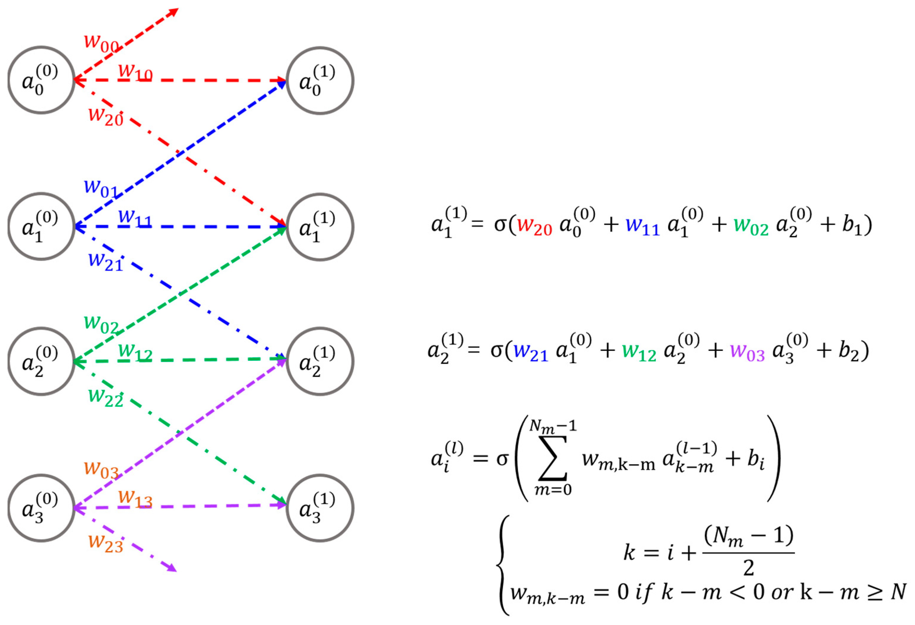
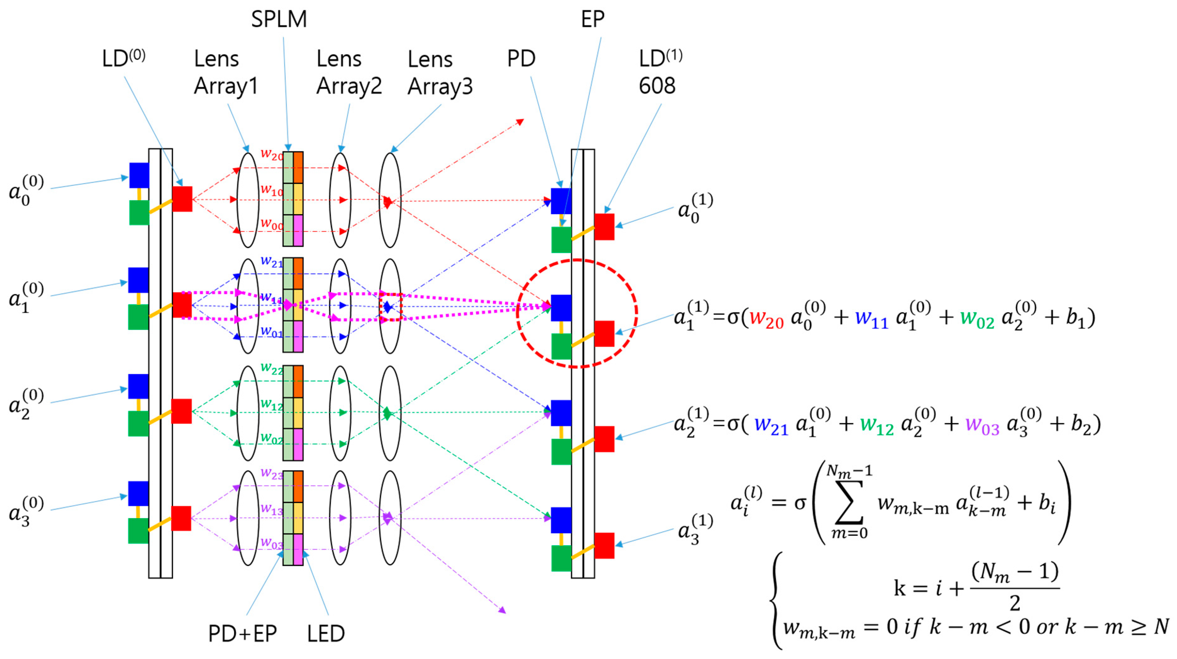
2.1. Fundamental Concepts of SPOCNN

To understand the structure of the proposed SPOCNN, it is essential to first grasp the fundamental principles of CNNs. Figure 1 presents a CNN example, showcasing four input and output nodes, their associated synaptic connections, and the mathematical formulation of these connections. A CNN functions by receiving signals at its input nodes, transmitting them through weighted synaptic connections to the output nodes, and then producing the final output. These synaptic weights, represented mathematically, determine the strength of each connection. Unlike fully connected optical neural networks like the LCOE, CNNs utilize localized or partial connections, where the weights assigned to these connections are referred to as kernels.
The previous SOCNN architecture [16] demonstrates outstanding optical parallelism and unlimited scalability of input node sizes with fixed weights, making it especially well-suited for inference tasks. However, it has limitations in applications that require processing identical input data with multiple weight sets due to its relatively slow update rate. While SLMs provide reconfigurability and programmability, their current switching speeds are restricted to a few kilohertz [14,15], leading to delayed computations and a significant reduction in throughput when weight updates are necessary during processing.
To overcome the limitations of SLMs in these scenarios, two possible solutions are available. The first is the development of a high-speed SLM system, including designs utilizing absorption modulators. However, this method requires significant time, resources, and financial investment. A more feasible alternative is to utilize existing technologies like smart pixels [20,21], which combine a detector, light source, and electronic processor (EP) within a single chip. Advances in optoelectronic integration have enabled the hybridization of these components into arrays. Additionally, the EP can serve multiple roles, including memory operations, making ONNs more programmable and intelligent than systems that rely solely on SLMs.
Figure 2 provides a visual representation of the SPOCNN concept introduced in this study. The CNN shown in Figure 1 has been transformed into a hardware implementation consisting of laser diodes (LDs), lenses, an SPLM, detectors, and supporting electronics. In this setup, each input node is replaced by an LD, which emits three light beams toward lens array 1. This setup allows for the integration of either a multimode vertical-cavity surface-emitting laser (VCSEL) or a light-emitting diode (LED) as the LD, as the system is designed to accommodate incoherent light sources—unlike the conventional 4f correlator system, which typically requires coherent light.
Lens Array 1 aligns the incoming light beams and channels them toward the SPLM, where each smart pixel alters the light intensity based on a pre-configured CNN kernel. The modified beams emerging from the SPLM then traverse Lens Array 2, which refocuses them and modifies their trajectories depending on the relative position of the SPLM pixels to the optical axis of each lens in the array.
A detector collects optical energy from beams arriving at different angles, emitted by multiple adjacent LDs or weighted input sources. The accumulated light output effectively corresponds to the convolution operation between the input signals and the predefined kernel weights. This architecture enables SPOCNNs to perform computations simultaneously and, critically, in a single step at the speed of light. This type of rapid computation aligns with what is termed “inference” in the neural network domain. The rapid reconfigurability of SPOCNNs makes them suitable for a wider range of applications beyond inference compared to SOCNNs.
In the optical system illustrated in Figure 2, Lens 2, and Lens 3 operate as a relay lens system. Typically, the SPLM is situated at the focal plane of Lens 2, while the detector is aligned with the focal plane of Lens 3. This configuration optically links the SPLM and detector planes, ensuring that each SPLM pixel is precisely mapped to a corresponding location on the detector. This conjugate relationship between the SPLM and detector allows for well-defined ray illumination, effectively reducing channel crosstalk.
Additionally, when an LD is positioned at the focal plane of Lens 1, the combination of Lens 1 and Lens 2 forms a relay lens system that projects an image of the LD onto Lens 3. The overall lens arrangement in Figure 2 functions as a Köhler illumination system [18,19]. In this setup, the magenta dotted lines indicate chief rays from the condenser’s viewpoint, while from the projection system’s viewpoint, they represent marginal rays. The red dotted rectangle near Lens 3 marks the location of the projected light source image. Within this Köhler illumination design, Lens 2 and Lens 3 together act as the projection lens system. The emitted rays from the LDs are evenly distributed across the detector plane, ensuring uniform illumination.
The SPOCNN architecture is fundamentally the same as the SOCNN [16], with the primary distinction being the use of SPLM instead of SLM. To achieve higher modulation speeds, multi-mode VCSELs can be used instead of LEDs, which have limited modulation capabilities [23,24,25]. The SPLM, illustrated in Figure 2, is composed of a photodetector (PD), an EP, and a LED. The PD receives incoming light, transforms it into an electrical signal, and forwards it to the EP within the SPLM. The EP processes this signal by adjusting its strength according to the weight value stored in its built-in memory. After amplification, the modified signal is transmitted to the LED, which emits light in proportion to both the input intensity and the assigned weight. Collectively, the PD, EP, and LED constitute a single functional unit called a smart pixel, where these units remain interconnected locally, except during the initialization phase when the program is being loaded. Once programmed, the pixel array operates independently, maintaining the system’s parallel processing capability. Each pixel essentially acts as a miniature signal repeater.
Thanks to its electronic components, the modulation speed of the SPLM surpasses several hundred megahertz, significantly outpacing typical SLM technologies such as liquid crystal displays and micro-electro-mechanical systems [14,15]. While the SPLM introduces two additional conversion steps—from optical to electrical signals and back to optical signals—, the resulting delay is minimal, totaling just a few nanoseconds [21]. Nevertheless, the substantial benefits of the SPLM’s high modulation speed far outweigh this minor delay, particularly in numerous practical applications, as discussed in the introduction.
The primary distinction between the SPOCNN and the earlier SPONN [22] lies in their connection structures. In the SPOCNN, each input is connected to a relatively small number of output nodes, whereas the SPONN employs a fully interconnected architecture. This feature of partial connectivity significantly alleviates limitations on the input array size. Unlike the conventional 4f correlator system, the SPOCNN does not impose a theoretical constraint on the size of the input array. However, the kernel array size is limited by the SBP constraints imposed by the imaging properties of the lenses used for SPLM pixel projection. This will be discussed in more detail in the discussion section.
In the configuration shown in Figure 2, the quantity of smart pixels linked to each input node matches the number of output nodes connected to that particular input. These smart pixels, organized into subarrays within the SPLM, correspond to the subarrays of the kernel. While the SPOCNN in Figure 2 is presented in a one-dimensional format, it can be readily expanded to a two-dimensional input-output arrangement. For example, if the subarray consists of a 3 × 3 pixel arrangement with a pixel spacing of d, and the detector spacing is b, the projection system’s magnification, given by as l3/l2, must match b/d. Here, l2 and l3 represent the distances from Lens 2 to the SPLM and from Lens 3 to the detectors, respectively.
If a single kernel spans an 8 × 8 pixel area on the SPLM, it can be connected to 64 output nodes. For example, an SPLM with a resolution of 3840 × 2160 pixels can support as many as 480 × 270 input nodes, corresponding to 129,600 inputs. Given the parallel processing capability of the SPOCNN, its performance is directly linked to the resolution of the SPLM. For a system with N × N inputs and an M × M kernel, the SPOCNN is capable of performing N2 × M2 multiplications and N2 × (M2 − 1) additions in one step. When the full resolution of the SPLM is utilized, (N × M)2 corresponds to the total number of available pixels. Furthermore, the high refresh rate of the SPLM—reaching several hundred megahertz [21]—makes the SPOCNN well-suited for applications requiring rapid weight updates. Additionally, since the SPLM transmission is directly proportional to the kernel weight, there is no need for additional Fourier transform calculations, unlike the 4f correlator system. This feature highlights the SPOCNN’s potential as a fast reconfigurable OCNN for future applications.
Once optical processing is complete, the detector transforms the incoming light into an electrical signal. The next stages, such as amplifying the signal, adding bias, and applying nonlinear operations (e.g., sigmoid, ReLU, local response normalization, and max-pooling), are performed electronically. Electronics are more effective for these nonlinear computations due to their inherent characteristics. However, to prevent interconnection bottlenecks, connections between distant electronic components should be minimized. As long as the electronics within the detector-side smart pixels remain localized and distributed, the system’s optical parallelism remains intact.
The SPOCNN features a cascading architecture, enabling seamless expansion along the beam propagation path. The output signal from each node is directly transmitted to the input of the next layer. Within this setup, each neuron in the artificial neural network consists of a detector, associated EPs, and a laser diode positioned in the subsequent layer. For a system with L layers, N2 × M2 × L computations can occur simultaneously in a single step, significantly boosting the SPOCNN’s throughput for continuous input.
Additionally, another distinction between SPOCNN and SOCNN is that the LED output in the SPLM emits diverging light, while the SLM preserves collimation. This effect can be reduced by positioning a small lens immediately after the LED. However, the diverging beam does not negatively impact SPOCNN performance. This is because the SPLM plane remains optically conjugate to the detector plane, aligned via Lens 2 and Lens 3. As a result, the LED’s image on the SPLM is precisely mapped onto the detector plane, irrespective of the LED’s divergence angle.

2.2. Simplifying SPOCNN with Electrical Fan-In and Fan-Out

The SPOCNN architecture can be further refined by substituting LD(0) and Lens 1 with an electrical fan-out, as illustrated in Figure 3a. A more detailed depiction of the electrical fan-out is provided in Figure 3b. In the initial design, the light source and Lens 1 act as an optical distributor for the input signal. In contrast, the electrical fan-out in Figure 3a,b functions as an alternative distributor within the electrical domain. This configuration utilizes a direct wiring scheme that links the output of the previous layer to the inputs of the SPLM pixels in the next layer. By implementing this approach, wiring complexity and electromagnetic interference are minimized, leading to a more streamlined and efficient system.
Eliminating LD(0) and Lens 1 not only streamlines the optical design but also removes the necessity for Köhler illumination. In the original setup, Köhler illumination relies on Lens 1 and Lens 2 functioning as a condenser system, while Lens 2 and Lens 3 form a projection system, as depicted in Figure 2. By discarding the condenser system and retaining only the projection system, the design can be further simplified, as illustrated in Figure 3a. In this modified configuration, Lens 2 and Lens 3 can be consolidated into a single optical element, which reduces spatial requirements and alleviates optical alignment difficulties. This integration also lowers costs and enhances overall system efficiency. Each layer of SPOCNN consists of an input smart-pixel array, a lens array, and an output detector array interfacing with a smart-pixel array. This simplified SPOCNN closely resembles the convolutional version of a lens array processor [26], with the key difference being the incorporation of smart pixels.
The replacement of SLMs with SPLMs offers substantial advantages by significantly simplifying the architecture and potentially lowering fabrication complexity and costs in the future. A 3D representation of the SPOCNN system is presented in Figure 3c. This modular architecture supports cascading and is well-suited for implementing multilayer OCNNs, similar to the LCOE design.

3. Results

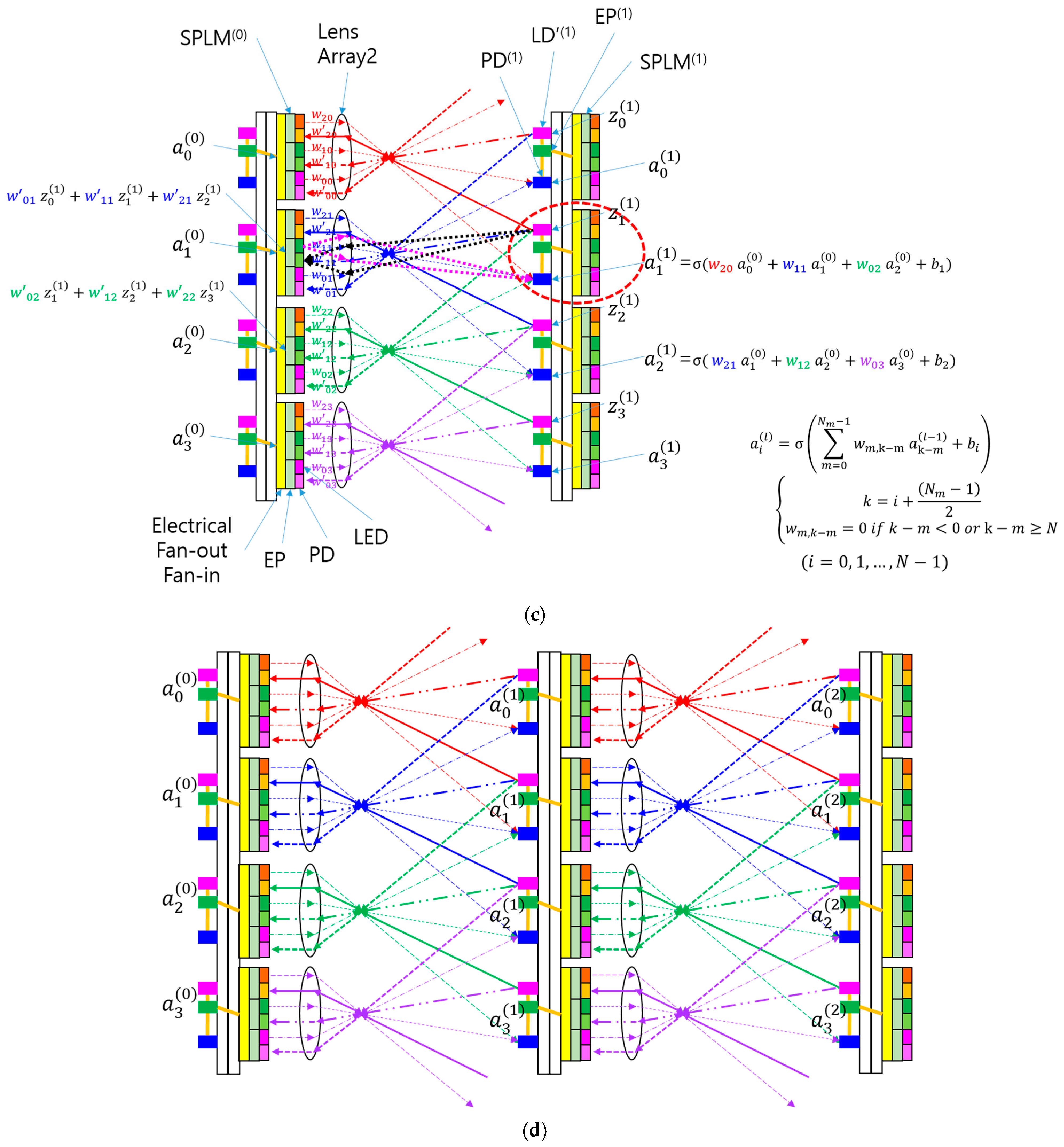
3.1. Smart Pixel-Based Bidirectional Optical Convolutional Neural Network (SPBOCNN)

The use of the SPLM instead of the SLM in an SOCNN [16] can also be adapted for application in BONN [23], as depicted in Figure 4a. In this SPBOCNN architecture, the SPLM takes over the role previously held by the SLM, modulating light traveling in both forward and backward directions based on the neural network’s weight values. With the help of Lens 2 and Lens 3, the SPLM pixels’ images are projected onto the detector plane or the second substrate, which also houses light sources ( L D 1 ( 1 ) ) to facilitate backward light propagation, as shown in Figure 4b. These backward light sources may consist of laser diodes combined with a grating and prism for beam property control. The beams passing through the SPLM are focused onto PDs ( P D 0 ( 0 ) ) on the first substrate, maintaining compatibility with the backward propagation process. Even with the replacement of the SLM by the SPLM, the core BONN structure remains intact, with a significant enhancement in modulation speed.
The SPLM’s ability to operate at modulation speeds of several hundred megahertz allows the neural network’s weight-refresh rates to reach similar levels [21]. The EP memory in the SPLM quickly sends updated weight values to the amplifier in just a few nanoseconds. This rapid weight-refresh capability overcomes the main limitations related to the slow modulation speed of SLMs in earlier BONN implementations. By introducing SPLM, practical realization of the backpropagation algorithm and the two-mirror-like BONN (TMLBONN) [23] configuration becomes feasible without requiring the development of new, high-speed SLM arrays. Detailed discussions on the implementation of backpropagation in BONN and the benefits of TMLBONN within this framework can be found in reference [23].
The SPLM employed in this BONN differs from those depicted in Figure 2 and Figure 3, with further details provided in Figure 4c. To achieve bidirectional modulation, the SPLM pixels are categorized into two distinct groups. One group is responsible for forward light propagation, containing PD1 on the left side and LED2 on the right side within the same pixel, interconnected by EP2. The second group handles backward propagation, where PD2, EP1, and LED1 are integrated within the pixel to control light in the reverse direction. Additionally, LED1 may be equipped with a microprism or lens to fine-tune beam divergence and emission angles, enhancing modulation control for bidirectional optical neural network functionality.

3.2. Simplifying SPBOCNN with Electrical Fan-In and Fan-Out

Similarly to the simplification process from Figure 2 and Figure 3, the SPBOCNN design in Figure 4 can be streamlined into the configuration shown in Figure 5a by replacing the optical input distribution, previously handled by Lens 1, with electrical fan-in and fan-out mechanisms. The refined SPBOCNN architecture, illustrated in Figure 5a, features an SPLM, lenses, smart pixels on the first substrate, and detectors positioned on the second substrate. While retaining bidirectional data flow, this design greatly simplifies the hardware.
An electrical fan-in is implemented to enable the analog summation of optical signals during backward data propagation, as shown in Figure 5b. The SPLM’s EPs transform the output signals into electrical current, which is then aggregated by the fan-in to the electrical input/output nodes of the EPs in the prior layer. Figure 5d presents a multilayer SPBOCNN, showcasing its cascading capability. This setup allows the addition of more layers to enhance parallel throughput for continuous input.
Just as Lens 2 and Lens 3 were combined into a single lens in the simplification depicted in Figure 3a, a similar reduction in optical components can be achieved with the SPBOCNN, as illustrated in Figure 5c. This integration minimizes space requirements and alleviates challenges related to optical alignment, contributing to lower costs and a more efficient system. Every layer of the SPBOCNN comprises a smart-pixel input array, a lens array, and a detector output array connected to another smart-pixel array.

3.3. Application of SPBOCNN in Difference Mode and Multiple Kernel Sets

In an SPBOCNN or SPOCNN, the addition of incoherent light by a detector and an SPLM cannot directly represent the negative weights of a kernel. While coherent light and interference effects could theoretically enable subtraction between inputs, using coherent light introduces complexities, including increased system noise and design challenges. Previous OCNN architectures, such as those based on the 4f correlator system [9], employed coherent light sources for SPLM emitters. However, as discussed in the introduction, coherent light sources bring inherent drawbacks like latency, noise issues, and limitations in cascading. To address the challenge of representing negative weights with incoherent light sources in this study, a ’difference mode’ is employed, as described in previous references [16,17,26].
Implementing the difference mode in SPBOCNN requires two distinct optical channels, similar to the approach used in SOCNN and LCOE [16,17]. One channel processes the input with positive weights, while the other handles the input with negative weights. Each channel uses optical methods to sum the weighted input values. The outputs from the two channels are then electronically subtracted, facilitated by communication between nearby electronic components. It is important to note that when one channel processes a nonzero weight, the corresponding weight in the other channel must be set to zero, ensuring no overlap.
However, SPBOCNN can simplify this process by eliminating the need for two separate optical channels. Instead, it utilizes the memory capabilities of smart pixels to perform the difference mode operation, as is the case with SPONN [22]. In SPBOCNN, inputs are first processed using positive weights, and the resulting outputs are stored in the smart pixel memory on the second substrate. Afterward, negative weights are introduced in place of the positive ones, prompting the system to recalculate the outputs. The results from the negative weights are then deducted from the previously stored outputs generated by the positive weights. While this method introduces a slight delay of a few tens of nanoseconds [21] due to the additional computation steps, it only needs half the number of output nodes compared to the conventional two-channel method.
This streamlined implementation is made feasible by the high weight-refresh rate of the SPLM, which minimizes the impact of the introduced delay. As a result, SPBOCNN can effectively perform the difference mode operation using a single optical channel, offering a practical and efficient solution when input and output node resources are constrained.
In fact, the same logic used for the difference mode in SPBOCNN can also be applied to cases where a single input dataset is convolved with multiple sets of kernels by utilizing the memory capabilities of smart pixels. In a previous study [16], multiple kernel sets were handled by assigning separate detector arrays to each Lens 3 in Figure 5a or Lens 2 in Figure 5c. This approach involved creating distinct optical channels for each kernel set, requiring a proportional increase in the number of smart pixels. However, SPBOCNN eliminates the need for additional optical channels by leveraging the memory of smart pixels, albeit with a slight increase in computation delay.
For instance, if there are four different kernel sets, the input data are first convolved with the initial kernel set, and the results are stored in the memory of the detector-side smart pixels. The system then updates the weight values in the SPLM to process subsequent kernel sets. Since the SPLM updates and the storage of outputs in detector smart pixels occur simultaneously and take less than 10 ns [21], the total computation time for one kernel set is approximately 20 ns. For four kernel sets, the computation would take 80 ns, compared to 20 ns in a previous OCNN system with four times the number of optical channels.
If this SPBOCNN were implemented using a traditional SLM, the computation delay would increase significantly—by a factor of 10,000—, resulting in 200 µs instead of 20 ns, while still requiring four optical channels, which would severely compromise optical parallelism. Therefore, SPBOCNN offers an efficient solution for processing multiple kernel sets, achieving substantial hardware savings with only a minor and tolerable delay.

4. Discussion

4.1. Scalibility of SPOCNN

While the SPBOCNN theoretically imposes no restrictions on the input array size, the scalability of the kernel size is constrained by Lens 2, as shown in Figure 5c. This limitation can be analyzed using the method described in previous studies [16,17], which involves assessing the dispersion of an SPLM pixel’s image through the projection system, considering geometric imaging, diffraction effects, and geometric aberrations. From this, one can determine the overlap of neighboring pixel images and the necessary alignment tolerances based on the calculated image dimensions.
To streamline this analysis, the architecture shown in Figure 3a was examined instead of the one in Figure 5. The scaling analysis of two systems are the same, except that the two optical channels of SPBOCNN corresponds to one channel of SPOCNN. The SPOCNN architecture features a two-dimensional (2D) input and output structure, combined with a four-dimensional (4D) kernel array. In this setup, the pixel counts for the input, SPLM, and output arrays are N2, N2 × M2, and N2, respectively, where N and M represent the number of rows in the square input array and the kernel array, respectively.
For scalability analysis, the densest component, the SPLM array, was prioritized in the design. A hypothetical system with a 5 × 5 kernel was analyzed. The SPLM pixels were assumed to have a square size of 5 µm and were arranged in a rectangular array with a period of 20 µm. According to the notations in Figure 3c, ε is 5 µm and d is 20 µm, respectively.
In this example, a 5 × 5 SPLM subarray receives an electrical input from a single node. Both the diameter of Lens 2 and the side length of the SPLM subarray were assumed to be 100 µm, as denoted by b in Figure 3c. This value also corresponds to the pitch of lens array 2 and the detector. With the SPLM and detector positioned at distances l1 and l2 from Lens 2, respectively, and satisfying their conjugate relationship, the SPLM pixel images are formed at the detector plane. Given that the detector pitch, b, is 5d, the projection system’s magnification must be 5. Generally, if the kernel’s array size is M × M, b equals Md, and the required magnification becomes M.
The projection system’s magnification is defined as the ratio l2/l1 = M. Thus, the geometric image size of a pixel, excluding aberration and diffraction effects, is Mε. With the SPLM pixel pitch scaled up to match the detector array pitch, the duty cycle of the SPLM pixel image remains constant at ε/d, equating to 25% of the detector pitch. Importantly, this duty cycle is unaffected by the kernel size, M.
Based on previous scaling analyses [16,17], the value of M can theoretically reach up to 66, which is sufficiently large for practical OCNN systems. The array size limit of 66 × 66 is based on the assumption that the f/# of Lens 2 is 2 and its angular aberration is approximately 3 mrad. However, this theoretical limit can be surpassed by using LCOE with clustering methods [17] or SPONN with software-based scaling [22]. While SPOCNN establishes only partial connections between the input and output arrays, LCOE and SPONN provide full connections. Therefore, the connections in SPOCNN can be considered a subset of those in LCOE or SPONN. This means that SPONN can emulate SPOCNN with the same number of inputs and outputs. Since fully connected ONNs are scalable through clustering and smart pixel memory, the limitations of SPOCNN can be effectively overcome.

4.2. A Design Example of SPOCNN

A design example of Lens 2 for SPOCNN is illustrated in Figure 6. The design was carried out using the optical design software CodeV (Ver. 2023.03) for an 850 nm wavelength, with optimization starting from a Cooke triplet. The entrance pupil diameter and magnification are 0.4 mm and 5.0, respectively. The kernel array size is 5 × 5, with dimensions of 0.200 × 0.200 mm2, allowing for a square pixel pitch and size of 40 µm and 10 µm, respectively. The distance from the center to the corner of the kernel array is 0.28 mm, which is why the three field points are set at 0.0, 0.2, and 0.3 mm.
Figure 6b shows the spot diagram with an Airy disk, indicating that the RMS spot size is much smaller than the diffraction spread. The combined effects of diffraction and geometric aberration are represented in the encircled energy diagram in Figure 6c, where 80% of the total energy falls within a circle with a diameter of 68 µm. Given that the kernel array image size or detector pitch is 200 µm, the diffraction and geometric aberration spot size accounts for 34% of the detector pitch, while the geometric image size of a single pixel is 50 µm (25%). The remaining 41% can be used for alignment tolerance in either the detector plane or the SPLM plane. In the SPLM plane, a 41% duty cycle corresponds to 16 µm, providing practical alignment tolerance using modern optical assembly techniques.
To examine the effect of increasing the kernel size, we increased the magnification to 11 by scaling up and re-optimizing the design. With this higher magnification, 80% of the total energy now falls within a 281 µm diameter, while the detector pitch increases to 440 µm. Since the pixel image size is 110 µm, the alignment tolerance is 49 µm at the detector plane and 4.5 µm at the SPLM plane. As magnification increases, greater design effort is required to maintain alignment tolerance, either by reducing the pixel duty cycle or applying different optimization rules.

4.3. Performance Analysis of SPOCNN Throughput

The parallel processing capability of the SPBOCNN is primarily determined by the size of the SPLM array. The SPLM array can be partitioned into smaller subarrays based on the kernel size [16]. A smaller kernel allows for a larger input array within a fixed SPLM array size. Additionally, the SPLM can be segmented to process multiple kernels simultaneously by replicating the input array across different sections. Each section of the SPLM can independently manage different kernels and carry out convolution in parallel [9].
In the SPBOCNN architecture, however, multiple kernels can be processed sequentially using the memory functionality of the SPLM, eliminating the need for separate optical channels for each kernel set. This design ensures that the number of operations per cycle corresponds to the total number of pixels in the SPLM. For instance, with an SPLM resolution of 3840 × 2160, approximately 8.3 × 10⁶ connections are achieved, enabling 8.3 × 10⁶ multiply-and-accumulate (MAC) operations per cycle. Assuming electronic processing is the primary source of delay—at around 10 ns [21]—, this system can deliver a computational throughput of 8.3 × 10¹⁴ MAC operations per second. Although the SPLM may have a delay of 10 ns, the kernel update can occur simultaneously with the signal processing at the smart pixels on the detector plane for continuous input, resulting in no additional delay.
The throughput can be enhanced further by stacking additional processing layers. While the addition of layers brings about extra data propagation delays, all layers operate in parallel, similar to pipelining in digital systems. With 10 layers, the system’s overall throughput could achieve an impressive 8.3 × 10¹⁵ MAC/s.
If the same input is convolved with 10 different kernel sets, the computations can be performed sequentially, moving from one set to the next without causing significant disruption to the operation. Simultaneously updating the kernel weights for the next layer and storing the outputs of the previous layer introduces a 10 ns delay, resulting in a total processing time of 10 ns per kernel set. Consequently, the overall throughput is 8.3 × 10¹⁵ MAC/s, despite the additional delay. However, this tradeoff eliminates the need for an SPLM array that is 10 times larger, significantly reducing system costs and increasing the flexibility of the OCNN.

4.4. Transverse Scaling of SPBOCNN Using Smart Pixel Memory

As mentioned earlier, SPBOCNN has no theoretical limitation on the size of the input array. However, increasing the input node size introduces significant challenges related to physical space, system flexibility, and manufacturing costs. Therefore, developing a software-based method for scaling the input node size is crucial for the practical implementation of SPBOCNN.
In the case of SPBONN [22], scaling was achieved by utilizing the memory capabilities of smart pixels, both on the SPLM and the detectors. Doubling the input and output nodes involved a nine-step process, which increased not only the time delay but also the throughput while enhancing system flexibility.
Similarly, scaling SPBOCNN can be accomplished by leveraging the memory of smart pixels at the input and output nodes, along with those in the SPLM, for rapid weight updates. The concept of SPBOCNN scaling is illustrated in Figure 7. The scaling direction is transverse, parallel to the plane of the neural network layer. Consider the entire rectangular region shown in Figure 7a as the total computation area for a given problem. This region can be divided into smaller dotted rectangular areas, referred to as elementary blocks, each of which can be processed by SPBOCNN hardware at a time, as shown in Figure 7b.
In this example, the SPBOCNN consists of input and output layers, as depicted in Figure 5c. The calculation begins in the top-left corner and shifts sequentially to neighboring blocks, following the yellow arrows in Figure 7a. For each elementary block, SPBOCNN performs convolution operations between the input and output nodes. When moving to the next block, the output is stored in memory, and the kernel, input, and output nodes are updated.
This process enables the system to scan the entire computation area. A key difference between SPBOCNN and SPBONN scaling is that SPBOCNN maintains partial connections between input and output nodes due to the nature of convolution, whereas SPBONN has fully connected nodes. This introduces more complex topological connections for SPBOCNN when transitioning between neighboring regions, as shown in Figure 7a.
For instance, consider an elementary block consisting of a 4 × 4 array with a kernel size of 3 × 3, as depicted in Figure 7b. In convolution, input nodes at the boundary of one block affect the output nodes at the boundary of the neighboring block, depending on the kernel size. In this example, the boundary nodes are influenced by neighboring blocks, and as the kernel size increases to 5 × 5, the interference extends to the second row from the boundary. As a result, calculating boundary nodes within a block requires information from the input nodes of the adjacent block.
This necessity is why boundary cells must be preserved when transitioning to the next block. Notably, the boundary cells retain their colors when shifting to neighboring blocks, as indicated by the yellow arrows in Figure 7a. The consistent color signifies that the same hardware input nodes are used for their calculation. Thus, transitioning between blocks is not a simple translational shift but rather a topological “flipping”.
Overall, all elementary blocks share the same color (or hardware input nodes) with neighboring blocks at their boundaries, forming a seamless connection similar to stitching patches. This ensures accurate convolution across blocks. Figure 7c illustrates the redrawn computation area with augmented boundaries, which includes a copy of the neighboring block’s boundary within each hardware block. In this manner, SPBOCNN scaling in the transverse direction can be achieved.
This approach offers a more flexible method for significantly increasing the input node size, depending on the available memory capacity.

4.5. Longitudinal Scaling of a Two-Mirror-like SPBOCNN

Scaling along the axis perpendicular to the layer plane can be achieved using a two-mirror-like SPBOCNN (TML-SPBOCNN), which serves as a smart pixel adaptation of TMLBONN [22,23] for convolution. As depicted in Figure 8, data reciprocates between two layers, enabled by the bidirectional nature and rapid reconfigurability of SPBOCNN, attributed to the memory-equipped smart pixels. This TML-SPBOCNN configuration can simulate 2n layers using only 2 physical layers, despite incurring a 2n-fold increase in time delay. For instance, while a 10-layer SPBOCNN reaches 8.3 × 10¹⁵ MAC/s, a 2-layer TML-SPBOCNN can reach 8.3 × 10¹⁴ MAC/s with a delay 10 times longer, while taking up one-tenth of the space and requiring five times fewer hardware resources. Consequently, TML-SPBOCNN offers a flexible approach to scaling the number of layers through software, which is a critical advantage during the early development phases. Its architecture demands much less hardware while simulating any number of layers, depending on the memory size of the smart pixels. In contrast, replacing the SPLM in TML-SPBOCNN with an SLM leads to a reduction in parallel throughput by a factor of at least 10,000, resulting in only 8.3 × 10¹⁰ MAC/s. Therefore, the benefits of using the SPLM in TML-SPBOCNN are clear.

4.6. Application of SPBOCNN in Solving Partial Differential Equations

An ideal demonstration of SPBCONN is its application in image classification, where instruction steps are analyzed based on the given hardware architecture, and throughput is measured along with processing delay. However, image classification requires not only the convolution process but also a fully connected process, along with data transfer control between these stages. This will be the focus of future research. Meanwhile, an intriguing and immediate application of TML-SPBOCNN is solving partial differential equations (PDEs). Many fundamental physical equations, such as the Poisson equation for gravity, Maxwell’s equations, the Schrödinger equation, and others, are expressed as PDEs. These equations depend on local interactions between neighboring cells when the computational domain is divided into discrete cells. For instance, the Laplace equation is shown in Equation (1), while its corresponding difference equation is presented in Equation (2), where i, j, and k represent the indices of 3-dimensional rectangular cells. According to Equation (2), the value of a particular cell is calculated as the average of its nearest neighboring cells. In the relaxation method [27], the function value at a specific position at time step t + 1 is computed using the neighboring values from time step t. With continued iterations, the value of each cell converges to the steady-state solution.
2 φ = 0
φ t + 1 i , j , k = 1 6 φ t i 1 , j , k + φ t i + 1 , j , k + φ t i , j 1 , k + φ t i , j + 1 , k + φ t i , j , k 1 + φ t i , j , k + 1
In general, these local interactions can be represented by the convolutions of a neural network. The steps performed by TML-SPBOCNN are illustrated in Figure 9. First, the convolution of the zeroth-layer and first-layer nodes is calculated and stored in the nodes on the opposite side, with data transfer occurring simultaneously in both directions using TML-SPBOCNN, as shown in Figure 9a. Second, copies of the zeroth and first layers are exchanged. Third, since the node values of the first layer are stored on the left side and the zeroth-layer values on the right during the second step, the convolution of the first layer on the left and the zeroth layer on the right is added to the previously stored values (indicated in red) on the opposite side. Fourth, the convolution of the second-layer and third-layer nodes is computed and stored in the layer on the opposite side, with data transfer occurring simultaneously in both directions. The convolution of the second layer is added to both the stored first-layer value (indicated in red) and the third-layer value. Similarly, the convolution of the third layer is added to the second-layer value and stored for the fourth-layer value (indicated in red). In this manner, the nodes in the first layer collect values from their neighbors in three dimensions, completing the local interactions for the first layer. For the remaining steps, the calculations repeat those shown in Figure 9a–c. The step shown in Figure 9d represents the first step of the second cycle.

5. Conclusions

SPOCNN was proposed to significantly improve the refresh rate of kernels in SOCNN by replacing the SLM with SPLM. It inherits the advantages of SOCNN—such as unlimited input node size, cascadability, and direct kernel representation—unlike a 4f correlator system. Additionally, the fast updating capability and memory of SPLM in SPOCNN enable numerous applications that require real-time updates without significant delay, such as convolution with multiple sets of kernels and difference mode.
SPOCNN was further simplified using electrical fan-out, allowing for the use of a single projection lens instead of three. This eliminates the optical alignment burden and reduces hardware fabrication costs.
SPOCNN evolved into SPBOCNN by adopting the bidirectional architecture concept of BONN. This SPBOCNN was then simplified further into a single lens-array optical system, replacing the three-lens-array optics, by utilizing electric fan-in and fan-out in the SPLMs.
The parallel throughput of SPBOCNN is proportional to the pixel count of the SPLM. For instance, with an SPLM resolution of 3840 × 2160, approximately 8.3 × 10⁶ connections are achieved, enabling 8.3 × 10⁶ MAC operations per cycle. Assuming electronic processing is the primary source of delay—around 10 ns—this system can achieve a computational throughput of 8.3 × 10¹⁴ MAC/s. In comparison, replacing the SPLM in SPBOCNN with an SLM reduces parallel throughput by at least 10,000 times, resulting in only 8.3 × 10¹⁰ MAC/s. Therefore, the advantages of using SPLM in SPBOCNN are clear.
The bidirectional functionality enables SPBOCNN to evolve into TML-SPBOCNN, facilitating data flow between two layers. The TML-SPBOCNN architecture can simulate 2n layers using just 2 physical layers, with a 2n-fold increase in time delay. For example, while a 10-layer SPBOCNN achieves a throughput of 8.3 × 10¹⁵ MAC/s, a 2-layer TML-SPBOCNN can achieve 8.3 × 10¹⁴ MAC/s while requiring ten times less space and five times fewer hardware resources. In this way, TML-SPBOCNN scales in the direction perpendicular to the layers.
Scaling of SPBOCNN is possible in the direction parallel to the layers. Notably, the elementary calculation block includes copies of neighboring cell values at the boundaries, allowing information to be gathered for convolution when transitioning between blocks.
Finally, TML-SPBOCNN was demonstrated to solve partial differential equations (PDEs) in physics. Since PDEs are based on local interactions between neighboring cells in three dimensions, they can be represented by a sequence of convolutions.
In this study, we propose SPOCNN and related architectures along with performance analysis. Due to the numerous advantages outlined, SPOCNN is anticipated to have a major impact on the future development of versatile convolutional neural network applications.

Funding

This research received no external funding.

Data Availability Statement

The datasets generated during and/or analyzed during the current study are available from the corresponding author on reasonable request.

Conflicts of Interest

The authors declare no conflicts of interest.

Abbreviations

The following abbreviations are used in this manuscript:
CNNConvolutional neural network
OCNNOptical convolutional neural network
GPUGraphics processing units
SBPSpace-bandwidth product
SLMSpatial light modulator
SOCNNScalable optical convolutional neural network
LCOELinear combination optical engine
SPOCNNSmart-pixel-based optical convolutional neural network
SPONNSmart-pixel-based optical neural network
SPLMSmart pixel light modulator
BONNBidirectional optical neural network
SPBOCNNSmart-pixel-based bidirectional optical convolutional neural network
TMLONNTwo-mirror-like optical neural network
VCSELVertical-cavity surface-emitting laser
LDLaser diode
LEDLight-emitting diode
PDPhotodetector or photodiode
EPElectronic processor
TMLBONNTwo-mirror-like BONN
TML-SPBOCNNTwo-mirror-like SPBOCNN
PDEPartial differential equation

References

  1. Hinton, G.; Deng, L.; Yu, D.; Dahl, G.E.; Mohamed, A.R.; Jaitly, N.; Senior, A.; Vanhoucke, V.; Nguyen, P.; Sainath, T.N.; et al. Deep neural networks for acoustic modeling in speech recognition: The shared views of four research groups. IEEE Signal Process. Mag. 2012, 29, 82–97. [Google Scholar]
  2. LeCun, Y.; Bengio, Y.; Hinton, G. Deep learning. Nature 2015, 521, 436–444. [Google Scholar] [PubMed]
  3. Lecun, L.; Bottou, L.; Bengio, Y.; Haffner, P. Gradient-based learning applied to document recognition. Proc. IEEE 1998, 86, 2278–2324. [Google Scholar]
  4. Chetlur, S.; Woolley, C.; Vandermersch, P.; Cohen, J.; Tran, J.; Catanzaro, B.; Shelhamer, E. cuDNN: Efficient primitives for deep learning. arXiv 2014, arXiv:1410.0759v3. [Google Scholar]
  5. Han, S.; Pool, J.; Tran, J.; Dally, W. Learning both weights and connections for efficient neural network. Adv. Neural Inf. Process. Syst. 2015, 28, 1135–1143. [Google Scholar]
  6. Rhu, M.; Gimelshein, N.; Clemons, J.; Zulfiqar, A.; Keckler, S.W. vDNN: Virtualized deep neural networks for scalable, memory-efficient neural network design. In Proceedings of the 2016 49th Annual IEEE/ACM International Symposium on Microarchitecture (MICRO), Taipei, Taiwan, 15–19 October 2016; pp. 1–13. [Google Scholar]
  7. Chen, T.; Moreau, T.; Jiang, Z.; Zheng, L.; Yan, E.; Shen, H.; Cowan, M.; Wang, L.; Hu, Y.; Ceze, L.; et al. TVM: An automated end-to-end optimizing compiler for deep learning. In Proceedings of the 13th USENIX Symposium on Operating Systems Design and Implementation (OSDI 18), Carlsbad, CA, USA, 8–10 October 2018; pp. 578–594. [Google Scholar]
  8. Jouppi, N.P.; Young, C.; Patil, N.; Patterson, D.; Agrawal, G.; Bajwa, R.; Bates, S.; Bhatia, S.; Boden, N.; Borchers, A.; et al. In-datacenter performance analysis of a tensor processing unit. In Proceedings of the 44th Annual International Symposium on Computer Architecture, Toronto, ON, Canada, 24–28 June 2017; pp. 1–12. [Google Scholar]
  9. Colburn, S.; Chu, Y.; Shilzerman, E.; Majumdar, A. Optical frontend for a convolutional neural network. Appl. Opt. 2019, 58, 3179–3186. [Google Scholar] [CrossRef] [PubMed]
  10. Chang, J.; Sitzmann, V.; Dun, X.; Heidrich, W.; Wetzstein, G. Hybrid optical-electronic convolutional neural networks with optimized diffractive optics for image classification. Sci. Rep. 2018, 8, 12324. [Google Scholar] [CrossRef] [PubMed]
  11. Lin, X.; Rivenson, Y.; Yardimci, N.T.; Veli, M.; Luo, Y.; Jarrahi, M.; Ozcan, A. All-optical machine learning using diffractive deep neural networks. Science 2018, 361, 1004–1008. [Google Scholar] [CrossRef]
  12. Sui, X.; Wu, Q.; Liu, J.; Chen, Q.; Gu, G. A review of optical neural networks. IEEE Access 2020, 8, 70773–70783. [Google Scholar] [CrossRef]
  13. Goodman, J.W. Introduction to Fourier Optics; Roberts and Company Publishers: Greenwood Village, CO, USA, 2005. [Google Scholar]
  14. Cox, M.A.; Cheng, L.; Forbes, A. Digital micro-mirror devices for laser beam shaping. In Proceedings of the SPIE 11043, Fifth Conference on Sensors, MEMS, and Electro-Optic Systems, Skukuza, South Africa, 8–10 October 2018; Volume 110430Y. [Google Scholar]
  15. Mihara, K.; Hanatani, K.; Ishida, T.; Komaki, K.; Takayama, R. High Driving Frequency (>54 kHz) and Wide Scanning Angle (>100 Degrees) MEMS Mirror Applying Secondary Resonance For 2K Resolution AR/MR Glasses. In Proceedings of the 2022 IEEE 35th Inter-national Conference on Micro Electro Mechanical Systems Conference (MEMS), Tokyo, Japan, 9–13 January 2022; pp. 477–482. [Google Scholar]
  16. Ju, Y.G. Scalable Optical Convolutional Neural Networks Based on Free-Space Optics Using Lens Arrays and a Spatial Light Modulator. J. Imaging 2023, 9, 241. [Google Scholar] [CrossRef] [PubMed]
  17. Ju, Y.G. A scalable optical computer based on free-space optics using lens arrays and a spatial light modulator. Opt. Quantum Electron. 2023, 55, 220. [Google Scholar] [CrossRef]
  18. Arecchi, A.V.; Messadi, T.; Koshel, R.J. Field Guide to Illumination (SPIE Field Guides Vol. FG11); SPIE Press: Bellingham, WA, USA, 2007; p. 59. [Google Scholar]
  19. Greivenkamp, J.E. Field Guide to Geometrical Optics (SPIE Field Guides Vol. FG01); SPIE Press: Bellingham, WA, USA, 2004; p. 58. [Google Scholar]
  20. Seitz, P. Smart Pixels. In Proceedings of the EDMO 2001/VIENNA, Vienna, Austria, 15–16 November 2001; pp. 229–234. [Google Scholar]
  21. Hinton, H.S. Progress in the smart pixel technologies. IEEE J. Sel. Top. Quantum Electron. 1996, 2, 14–23. [Google Scholar] [CrossRef]
  22. Ju, Y.-G. A Conceptual Study of Rapidly Reconfigurable and Scalable Bidirectional Optical Neural Networks Leveraging a Smart Pixel Light Modulator. Photonics 2025, 12, 132. [Google Scholar] [CrossRef]
  23. Ju, Y.G. Bidirectional Optical Neural Networks Based on Free-Space Optics Using Lens Arrays and Spatial Light Modulator. Micromachines 2024, 15, 701. [Google Scholar] [CrossRef] [PubMed]
  24. Feng, M.; Wu, C.-H.; Holonyak, N. Oxide-Confined VCSELs for High-Speed Optical Interconnects. IEEE J. Quantum Electron. 2018, 54, 2400115. [Google Scholar] [CrossRef]
  25. James Singh, K.; Huang, Y.-M.; Ahmed, T.; Liu, A.-C.; Huang Chen, S.-W.; Liou, F.-J.; Wu, T.; Lin, C.-C.; Chow, C.-W.; Lin, G.-R.; et al. Micro-LED as a promising candidate for high-speed visible light communication. Appl. Sci. 2020, 10, 7384. [Google Scholar] [CrossRef]
  26. Glaser, I. Lenslet array processors. Appl. Opt. 1982, 21, 1271–1280. [Google Scholar] [CrossRef] [PubMed]
  27. Available online: https://en.wikipedia.org/wiki/Relaxation_(iterative_method) (accessed on 17 March 2025).
Figure 1. Illustration of a basic CNN along with its mathematical representation: a i ( l ) denotes the i-th node in the l-th layer, while w i j represents the weight linking the j-th input node to the i-th output node. b i denotes the bias associated with the i-th node. N corresponds to the input array size, whereas Nm specifies either the kernel size or the number of weights linked to each node. The function σ represents the sigmoid activation function.
Computers 14 00111 g001
Figure 2. An example of an SPOCNN utilizing free-space optics with lens arrays and an SPLM: Schematic representation and corresponding mathematical formula. The SPLM used in the SPOCNN includes smart pixels comprising a photodetector (PD), electronic processing (EP), and a light-emitting diode (LED). The smart pixels receive light input and emit output light proportional to the weight value stored in the EP memory. The LD can be either a laser diode or an LED.
Computers 14 00111 g002
Figure 3. The simplified version of the SPOCNN utilizing electrical fan-out: (a) Schematic representation and corresponding mathematical formula. Additionally, Lens 2 and Lens 3 in Figure 2 are combined into a single lens. (b) The SPLM used in the SPOCNN, where the electrical fan-out connects the input nodes to individual pixels in the SPLM. EP represents the electronic processor for each pixel, which includes memory and is connected to the LED output. (c) A three-dimensional view of the system with 3 × 3 inputs and 3 × 3 outputs. Ε represents the size of the light source in the SPLM, while b, and d indicate the spacing between detectors (or subarrays) and smart pixels, respectively. L1 and l2 denote the distances from Lens 2 to the SPLM and the detector, respectively.
Computers 14 00111 g003
Figure 4. An example of an SPBOCNN: (a) A diagram of the SPBONN along with the corresponding mathematical formulas. a i ( l ) denotes the i-th input or output node in the l-th layer. w j i signifies the weight linking the i-th input to the j-th output in the forward direction, while w j i represents the weight in the backward direction. The thin lines represent the light paths in the forward direction, while the thick lines represent those in the backward direction. (b) Light source dedicated to the backward direction. (c) Diagram of the smart pixel light modulator utilized in the SPBOCNN.
Computers 14 00111 g004
Figure 5. A further simplified version of the SPBOCNN, utilizing free-space optics, lens arrays, and an SPLM with electrical fan-in and fan-out: (a) Diagram of the SPBOCNN incorporating electrical fan-in and fan-out. (b) Illustration of the electrical fan-in and fan-out applied to the output and input of the SPLM. (c) Further simplification by combining Lens 2 and Lens 3 into a single lens. w j i represents the weight linking the i-th input to the j-th output, while w j i represents the weight in the backward direction. The thin lines indicate the light paths in the forward direction, while the thick lines indicate those in the backward direction. (d) An example of a multilayer SPBOCNN.
Computers 14 00111 g005aComputers 14 00111 g005b
Figure 6. A design example of Lens 2 for SPOCNN with a kernel size of 5 × 5, based on a Cooke triplet at 850 nm: (a) Lens layout; (b) spot diagram with a circle indicating the Airy disk; (c) diffraction encircled energy.
Computers 14 00111 g006aComputers 14 00111 g006b
Figure 7. An example of scaling the SPBOCNN in the direction parallel to the layer using the stitching method and the memory of smart pixels is as follows. (a) The original calculation area is divided into an array of sectors. Each sector, indicated by dotted lines, is processed by the SPBOCNN hardware one at a time, while the yellow arrows indicate the sequence of calculations. (b) A period of the cells or an elementary block, as calculated by SPBOCNN hardware. (c) The calculation area is redrawn with augmented boundary cells that contain copies of the boundaries of the neighboring sectors, as the SPBOCNN hardware requires information from neighboring sectors for convolution calculations. The yellow arrows indicate the sequence of calculations when the SPBOCNN hardware scans the entire calculation area using the stitching method.
Computers 14 00111 g007
Figure 8. An illustration of a TML-SPBOCNN: The data move reciprocally between the two layers, following the sequence outlined by the arrows above the diagram, simulating the functionality of a multilayer neural network.
Computers 14 00111 g008
Figure 9. An example of applying the TML-SPBOCNN to a partial differential equation (PDE) solving problem. (a) The convolution of the zeroth-layer and first-layer nodes is calculated and stored in the nodes on the opposite side, with data transfer occurring simultaneously in both directions. (b) Copies of the zeroth and first layers are exchanged. (c) The convolution of the first layer on the left and the zeroth layer on the right is added to the previously stored values (indicated in red) on the opposite side. (d) The convolution of the second-layer and third-layer nodes is calculated and stored in the layer on the opposite side, with data transfer occurring simultaneously in both directions. The convolution of the second layer is added to both the stored first-layer value (indicated in red) and the third-layer value. Likewise, the convolution of the third layer is added to the second-layer value and stored for the fourth-layer value (indicated in red). In this manner, the nodes in the first layer collect values from their neighbors in three dimensions, completing the local interactions required for PDE solving.
Computers 14 00111 g009aComputers 14 00111 g009b
Disclaimer/Publisher’s Note: The statements, opinions and data contained in all publications are solely those of the individual author(s) and contributor(s) and not of MDPI and/or the editor(s). MDPI and/or the editor(s) disclaim responsibility for any injury to people or property resulting from any ideas, methods, instructions or products referred to in the content.

