A Review of Vessel Time of Arrival Prediction on Waterway Networks: Current Trends, Open Issues, and Future Directions

Abstract

With the vast majority of global trade volume and value reliant on maritime transport, accurate prediction of vessel estimated time of arrival (ETA) is crucial for optimizing supply chain efficiency and managing logistical complexities in port operations. This review paper systematically examines the current state of research and practices in the field of vessel ETA prediction, highlighting significant trends, methodologies, and technologies. It explores various approaches, including classical methods, machine learning and deep learning algorithms, and hybrid methods, developed to enhance the accuracy and reliability of vessel travel time and arrival time predictions. Additionally, this paper categorizes key influencing factors and metrics, and identifies open issues and challenges within current prediction models. Concluding with proposed future research directions aimed at addressing the identified gaps and leveraging technological advancements, this review emphasizes the importance of fostering innovation in maritime ETA prediction systems, particularly within the framework of Intelligent Transportation Systems (ITSs) and maritime logistics. By applying a systematic literature review (SLR) methodology and conducting an in-depth evaluation, the results provide a comprehensive overview of vessel ETA prediction for researchers, practitioners, and policy makers involved in maritime transport and logistics, and offer insights into the potential for improved efficiency, safety, and environmental sustainability in waterway networks.

1. Introduction

Maritime transport plays a significant role in global supply chains, accounting for 80% of the volume and 70% of the value of traded goods worldwide [1]. The arrival of ships at ports profoundly impacts all subsequent processes of the supply chain [2] and plays a central role in addressing the primary planning and scheduling challenges at container terminals [3,4]. As vessel traffic intensifies, particularly in ports where multiple harbor basins share a restricted channel, traffic conflicts and vessel delays frequently occur [5]. Port terminals, in particular, bear the burden of this uncertainty, as the need to plan berth allocation often results in either fully occupied berths due to early vessel arrivals or wasted resources when vessels are delayed. Both scenarios have a negative economic impact, affecting not only terminals, but also ship owners and the entire supply chain. The utilization of advanced technologies for the accurate prediction of vessel estimated time of arrival (ETA) is imperative for enhancing the sustainability of logistics operations. This approach significantly contributes to the economic sustainability of the supply chain, thereby underscoring its critical role in the optimization of maritime operations. Reliable vessel ETA can assist port stakeholders, including businesses, planners, and policy makers, in effectively managing the complexities associated with logistical challenges, which contributes to the overall efficiency and effectiveness of supply chain operations. Recent developments in Intelligent Transportation Systems (ITSs) have led to the widespread implementation of AI algorithms and technologies in waterborne transport that address the identified problems in predicting vessel ETA. However, despite the progress made in data modeling techniques, such as machine learning and deep learning algorithms, and the capability to handle large datasets, several critical issues still need to be solved in ETA prediction. Therefore, it is important to identify and address these existing shortcomings and comprehensively analyze the current state of the art in vessel ETA prediction.

This study presents a systematic literature review (SLR) to obtain a comprehensive understanding of ETA modeling used in the waterway network. The purpose of this study is to (i) provide a comprehensive overview of different methods used in order to identify deficiencies and drawbacks in ETA prediction modeling for waterborne transportation; (ii) categorize these methods, explain key concepts, analyze factors impacting ETA, and evaluate various metrics used in ETA modeling; (iii) identify open issues related to ETA prediction modeling; and (iv) discuss potential future improvements to enhance the effectiveness of existing approaches.

There is a lack of studies explicitly dedicated to reviewing the literature on ETA prediction within waterway networks, encompassing both sea and inland routes. Sea waterways, such as the North Sea routes, are large bodies of salt water that connect continents and countries, and are typically deeper and wider than inland waterways. Inland waterways, which include rivers, canals, and lakes within a country or between neighboring countries, are generally smaller and shallower. They can be divided into natural inland waterways, such as the river Rhine or the river Weser, and artificial waterways, such as the Mittellandkanal, which have been constructed to improve navigability or provide logistical shortcuts. Figure 1 shows a North Sea route through which a ship can travel from the Bremerhaven port in Germany to the Rotterdam port in the Netherlands. Additionally, in the same figure, a ship can travel from Braunschweig to Minden via the artificial waterway the Mittellandkanal, and then from Minden to Bremerhaven through the natural inland waterway river Weser. Dobrkovic et al. [2], who analyzed existing methods and algorithms for predicting maritime routes using Automatic Identification System (AIS) data from 2004 to 2015, did not focus specifically on ETA. This study categorized the publications according to three prediction objectives (trajectory, arrival time, and route variation), prediction methods, timeframe, accuracy, and data quality. The study presented here makes a noteworthy contribution compared to the previously mentioned paper for the following reasons:

(i)

It is one of the initial efforts to specifically focus on vessel ETA, including estimated time of arrival, travel time, and time of arrival. This study does not focus solely on a single aspect of relevant methods, such as machine learning. Instead, it provides a comprehensive analysis of several approaches by presenting a taxonomy. Additionally, this study offers comparative data on methodologies, evaluation metrics, etc.

(ii)

This review highlights various factors that influence ETA models and the different performance metrics used to evaluate them.

(iii)

This research also summarizes the open issues with existing vessel ETA prediction models.

The subsequent sections of this document are organized as follows: Section 2 outlines the specific questions investigated, the criteria used for selecting relevant information, and the systematic process employed for conducting the search. Section 3 is divided into three sub-sections: ETA methods, included factors, and evaluation metrics. This paper discusses the methodology and challenges associated with modeling and prediction in Section 4. Finally, this report examines the primary findings and limitations of this study, while also offering broad recommendations.

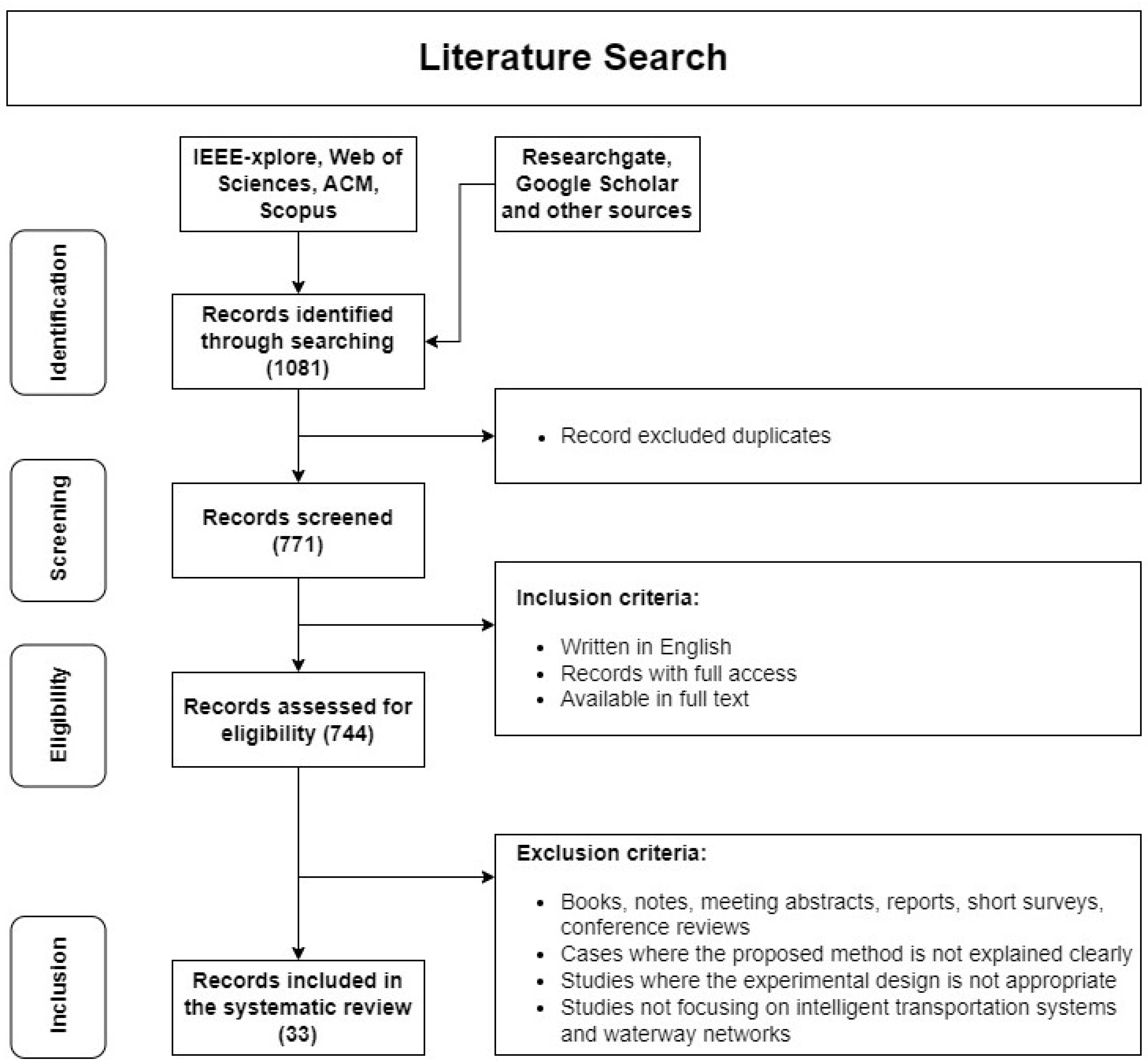
2. Research Methodology

An SLR is a method used to systematically analyze and synthesize existing research relevant to a set of research questions. Its purpose is to identify gaps in current research and propose areas requiring further exploration [6,7]. The PRISMA guidelines were utilized to conduct and report this review activity [8]. The subsequent sections provide a comprehensive examination of the formulated review method, encompassing the research inquiries, the criteria and process for selection, the search strategy, and the presentation manner.

2.1. Research Questions

To accomplish the objectives of this study, the following research questions (RQs) were devised:

• RQ1. What methodologies are currently employed for predicting ETA on waterways?
• RQ2. Which are the evaluation metrics and factors for ETA modeling in waterway transportation?
• RQ3. What are the open issues related to ETA prediction modeling?
• RQ4. Which research opportunities can be emphasized for future investigation?

The first two questions are addressed in Section 3. Section 4 presents a comprehensive summary of the problems related to current ETA modeling, addressing RQ3. Section 5 explores potential avenues for future research, as outlined in RQ4.

2.2. Search Query String

A comprehensive search was conducted across several databases, including IEEE Xplore, ACM Digital Library, Scopus, and Web of Science, to identify relevant studies. These databases appeared to be relevant and comprehensive for ITS research. The search included journal articles and conference proceedings from 2011 to 2023. A list of key terms and their synonyms, such as “arrival time”, “journey time”, “travel time”, “ETA”, “ship”, “vessel”, etc., was compiled. These terms were used to create inclusive and relevant queries through several iterations. Boolean operators “OR” (to include synonyms and alternative terms) and “AND” (to link different search terms) were used in the search query. The search query for this study is as follows: ((“travel time” OR “journey time” OR “arrival time” OR “time of arrival” OR “eta” OR “estimate* time”) AND (“predict*” OR “estimate*” OR “forecast*”) AND (“ship*” OR “vessel*” OR “voyage”)).

2.3. Study Selection and Quality Assessment

During this phase of the review, the collected papers were studied by examining the title, abstract, methodology, and conclusion. Inclusion and exclusion criteria were applied to filter out unnecessary papers based on their titles and abstracts. Eligible articles were those meeting at least one inclusion criterion, while manuscripts meeting any exclusion criterion were excluded (

Table 1. Research article inclusion and exclusion criteria.

Inclusion Criteria	Exclusion Criteria
Only publications in English and accessible in their full length are included in the analysis.	Duplicate reports of the same study, retain only the most complete version or the most recent report.
An algorithm for modeling ETA must be included in the paper.	Abstracts, editorials, books, notes, conference reviews and unpublished material.
The paper has to provide an answer to at least one of the research questions.	Insufficient detail to understand the experiment architecture and design.

).

Furthermore, quality assessment criteria were considered to select articles that might offer reliable and the best responses to the research questions and the criteria discussed earlier. This study evaluated the reliability and quality of the selected papers based on the following criteria:

• Does the research provide a concise and explicit statement outlining its goals, purposes, challenges, objectives, and questions?
• Is the proposed methodology for ETA on waterway networks adequately explained?
• Is the experimental design suitable?

The following section outlines the procedures involved in the selection process and the resulting number of studies that were chosen after applying the qualifying criteria. A total of 1081 papers were found in the identification phase. Figure 2 depicts the literature selection process, which encompasses identification, screening, eligibility, and analysis. It also presents the number of article modifications that occur at each stage of the process. A total of 310 papers were excluded based on title examination, primarily due to issues such as duplication and non-English language. Thus, there were 744 papers left for further selection. After conducting a more thorough evaluation by exploring the titles and abstracts of these 744 papers, it was determined that 711 of them did not meet the criteria and were, therefore, excluded. Ultimately, the process of manual selection yielded a total of 33 papers that met the criteria for inclusion in the systematic review.

2.4. Data Collection and Synthesis

The data collected in the SLR are the results obtained from individual research studies relevant to the research issue. The primary objective of this step is to gather and combine data and evidence from the selected documents to address the research inquiries. The extracted data from each study include general information such as the authors of the paper, the year of publication, the methodology suggested by the authors, and the challenges associated with ETA modeling as well as the factors, experimental setting, and results of evaluating the performance of the proposed approach.

Table 2. Overview of articles based on the algorithms, used factors, and evaluation metrics.

Article	Used Algorithms	Best Algorithm	Data Source	Factors Used in ETA Modeling	Performance Metrics
[9]	Path-Finding		AIS, LRIT
[10]	MLP	MLP	AIS
[11]	Venilia	Venilia	AIS	Vessel name, Vessel type, Speed, Course over ground, Heading, Source port, Draught, MMSI, Direction of the vessel trajectory, Direction pointed by the vessel bow, Event timestamp, Reported source port name
[12]	Transformer, MLP, CNN, LSTM, BiLSTM	BiLSTM	AIS	Trip identification number, Latitude of the next vessel position, Longitude of the next vessel position, Distance between current and next position, Maximum draft, Current draft, Vessel length, Vessel width, Deadweight tonnage, Net tonnage, Gross tonnage, Maximum power, Age of the vessel, Vessel type	R2, RMSE, MAE, MSE
[13]	RF, CART, BLR, MLP	RF	AIS		Bias, MAD, MAE, MAPE, MSE, RMSE
[14]	NN, LSTM, RNN, GRU	NN	AIS, LRIT, TOS		MAE, MSE
[15]	NN, SVR, RF, GB, RR	NN	AIS	Speed over ground, Course over ground, Heading, Origin and destination port coordinates	MAE, MSE
[16]	MLP, LSTM, 1D-CNN, WaveNet	LSTM	AIS	Speed over ground, Course over ground, Heading, Navigational status, Draught, Zonal ocean current velocity, Meridional ocean current velocity, Sea surface temperature, Significant height of combined wind waves and swell, Mean wave period, Mean wave direction, 10 m U-component of wind, 10 m V-component of wind, Gross tonnage, Deadweight, Length, Beam, Year built, Vessel type, Trajectory origin latitude, Trajectory origin longitude, Route leg distance, Route leg speed, Accumulated distance, Remaining distance	MAE, MSE
[17]	NN	NN		Ship name, Ship length, Transit time, Number of dockers required for unloading, Number of dockers required for loading, ETA month, ETA day of the week, ETA hour	APE
[18]	Path-Finding, SVR, LSTM, VCIN	VCIN	AIS		MAE, MAPE, RMSE
[19]	SVR, GBT, KNN, RF, XGBoost, SE –ResNext, LightGBM	SE –ResNext	GPS		MAE
[20]	ANN	ANN	AIS	Length, Breadth, Draught, Wind speed, Water Depth, Sea state
[21]	LR, KNN, DTR, ANN	ANN			MAE, R2, MAPE, RMSE
[22]	Path-Finding	Path-Finding	AIS		APE
[23]	DNN, RNN, LR	DNN	AIS	Vessel type, Speed, Course over ground, Cumulative distance, Cumulative time, Heading, Bearing	MAE
[24]	LSTM, GRU	GRU	AIS		Perplexity Score
[25]	GBDT, MLP, GRU	GRU			MAE, RMSE
[26]	Bayesian Approach			Wave height, Wave period, Wind speed, MMSI, Speed over ground, Course over ground, Heading, Significant wave height, Primary wave mean period, Primary wave direction, North–south wind component, East–west wind component	MAPE
[27]	CART			ETA at pilot point, ATA at pilot point, Length, Gross tonnage, Capacity, Vessel type, Previous port, Shipping line, Service, Sailing direction, Average speed, Delay, Previous port distance, Sailing
[28]	LR, CT, RF	RF		Length, Gross tonnage, Capacity, Vector type (mother/feeder), Owner’s name, Owner’s frequency, Port rotation, Sailing direction, ETA at the pilot point, ATA at the pilot point, Presence of a lock before reaching the terminal, Wind speed
[29]	Path-Finding		AIS
[30]	ANN	ANN	AIS		MAE, MAPE
[31]	Nearest Route Points Search	Nearest Route Points Search
[32]	FRBBN	FRBBN	AIS
[33]	XgBoost, SVR			Average vessel speed, Standard deviation of vessel speed, Lock delay statistics, River level conditions	MAPE, RMSE
[34]	ExtraTrees, AdaBoost, SVR	SVR		Unit load identifier, Start/end of tracking, Gateway identifier, Temperature, Humidity, Crafted features	MAE, RMSE
[35]	Process Mining		AIS	Port ETA agent, Pilot board at vessel, Approach area ATA vessel, Port ATA vessel, Berth ATA vessel, Pilot switch, Tug standby at vessel, Lock ATA vessel, Lock ATD vessel, Port ETD agent, Anchorage area ATD vessel, Anchorage area ATA vessel, First line secured at vessel, Last line secured at vessel, ETA at pilot point, Berth ATD vessel
[36]	Bayesian Approach		AIS
[37]	NN	NN		MMSI, Status of the vessel (underway, moored, etc.), Speed over ground, Course over ground, Heading, ETA, Destination (manual input from the skipper), Draught	MAE, MRE, RMSE
[38]	Self-Developed Algorithm		AIS	Type of a vessel, Width of a vessel, Draft of a vessel, Time of day
[39]	Self-Developed Algorithm		PORT-MIS, TOS	Vessel name, API call timestamp, Heading, ETA, Destination, Speed over ground, Ship arrival and departure declaration system from Port-MIS system, TOS berth plan	MAE, MAPE, RMSE
[40]	MLP, CART, RF			Vessel name, Vessel type, Length, ETA, ATA, Vessel service route type (trunk/external feeder/internal feeder/barge feeder/domestic trade line)
[41]	LSTM, BiLSTM, GRU, LSTM-KF	LSTM-KF	AIS		MAE, RMSE

displays the distribution of the chosen papers obtained in this study, excluding any duplicates or irrelevant papers. Moreover, this table includes the following fields: the reference, implemented methodologies, evaluation criteria, and the influential factors. Some terms are defined below, which will be used throughout the rest of this paper.

• Long-Range Identification and Tracking (LRIT);
• Global Positioning System (GPS);
• Multi-Layer Perceptron (MLP) and Artificial Neural Network (ANN);
• Deep Neural Network (DNN);
• One-Dimensional Convolutional Neural Network (1D-CNN);
• Recurrent Neural Network (RNN);
• Long Short-Term Memory (LSTM);
• Bidirectional Long Short-Term Memory (BiLSTM);
• Gated Recurrent Unit (GRU);
• Random Forest (RF) and Classification Tree (CT);
• Classification and Regression Tree (CART);
• Gradient Boosting Decision Trees (GBDTs);
• eXtreme Gradient Boosting (XGBoost);
• Bayesian Linear Regression (BLR) and Ridge Regression (RR);
• Fuzzy Rule-Based Bayesian Network (FRBBN);
• Squeeze-and-Excitation ResNeXt (SE-ResNext);
• Variable Coefficient Inference Network (VCIN);
• Support Vector Regression (SVR);
• K-Nearest Neighbors (KNN) and Kalman Filter (KF);
• Absolute Percentage Error (APE) and Mean Absolute Error (MAE);
• Mean Squared Error (MSE) and Perplexity Score (PS);
• Root Mean Squared Error (RMSE)
• R-squared (R2) and Mean Absolute Deviation (MAD);
• Mean Relative Error (MRE);
• Mean Absolute Percentage Error (MAPE);
• Maritime Mobile Service Identity (MMSI);
• Application Programming Interface (API);
• Port Management Information System (PORT-MIS);
• Terminal Operating System (TOS);
• Actual Time of Arrival (ATA);
• Actual Time of Departure (ATD);
• Estimated Time of Departure (ETD).

3. Analysis and Discussion

The purpose of this section is to address the RQ1 and RQ2 outlined in Section 2. This research specifically examines the methodologies used for ETA on waterways, categorizes different methodologies, and highlights the primary challenges associated with each category. Additionally, a comprehensive summary of each work is provided, including a variety of evaluation metrics, factors considered, and descriptions of the primary concepts. This information is presented in Table 2. In the following subsections, (1) the presented methods for modeling ETA on waterway networks (RQ1) are examined in Section 3.1; (2) factors involved in ETA modeling (RQ2) are discussed in Section 3.2; and (3) the evaluation metrics (RQ2) are detailed in Section 3.3.

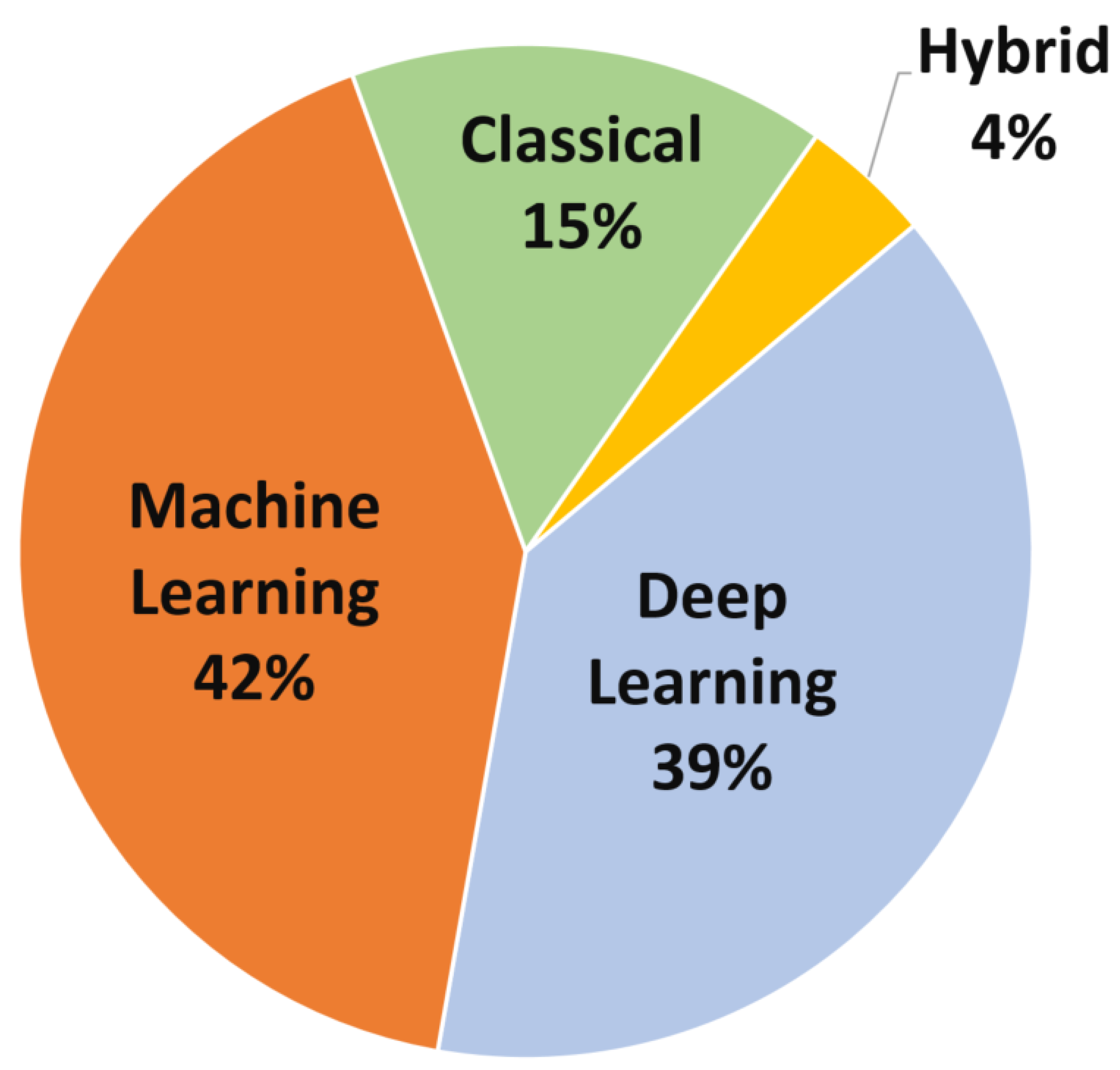
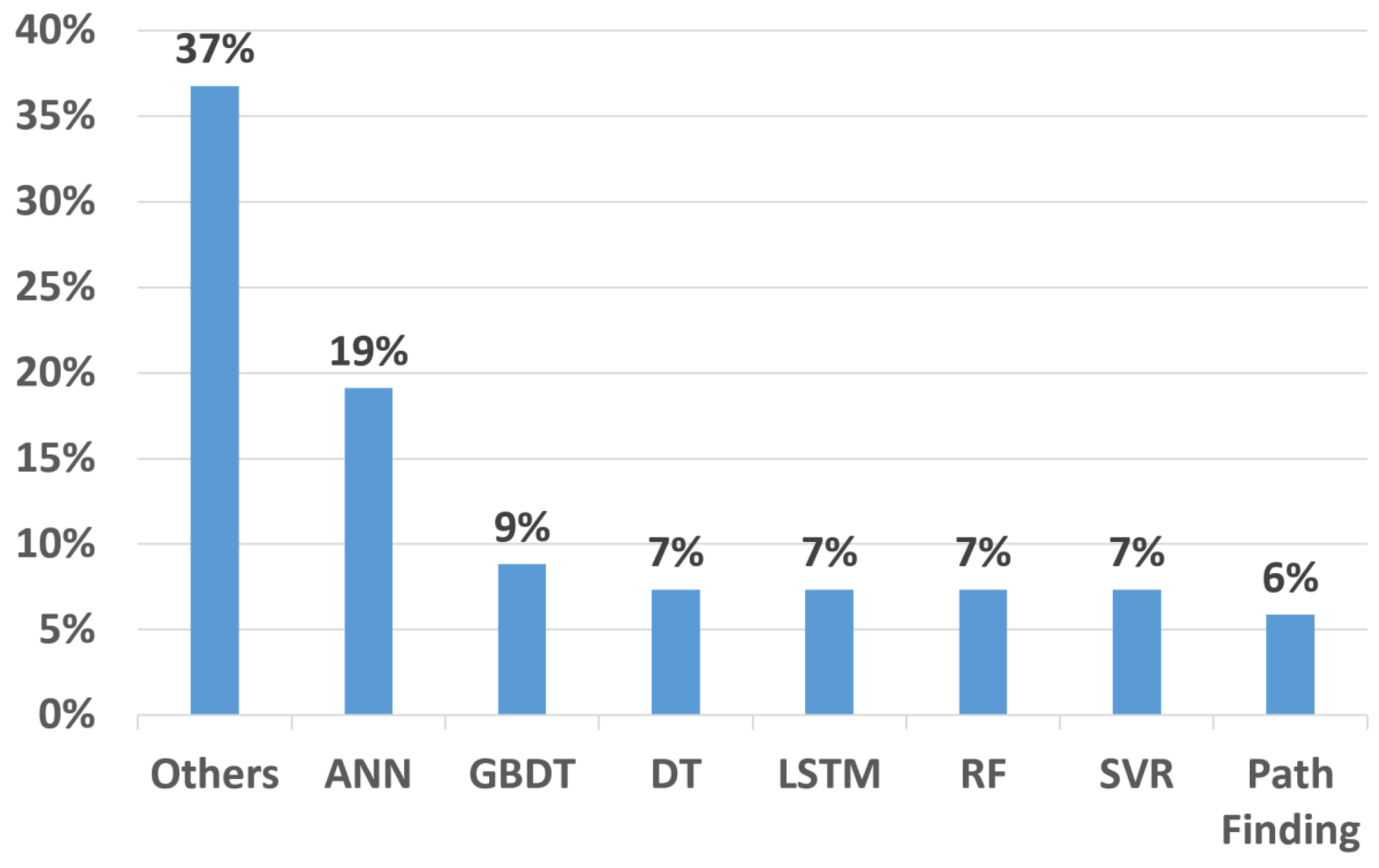
3.1. Taxonomy of the ETA Methods

The results of this review indicate that current methods can be classified into four main categories according to the characteristics of the implemented algorithms. Classical methods, shallow machine learning methods, deep learning methods, and hybrid methods are the four approaches. A brief overview of the four categories is given below, along with a synopsis of the methods used in each category to predict ETAs.

3.1.1. Classical Methods

Various classical methods are used to predict the ETA of a given period based on observed historical data from previous trips during the same period. These methods are widely used in practice due to their effective data filtering, minimal computation time, and ease of implementation. However, the overall performance of these models is inadequate due to the fact that a classical method can only be considered reliable under the assumption that the navigational factors are constant. Consequently, the accuracy of classical methods is compromised by any change in waterway navigation factors, including extreme weather events or accidents.

The Bayesian Approach is a probabilistic method used for making predictions and estimating parameters. It relies on Bayes’ Theorem, which updates the probability of a hypothesis as more evidence or information becomes available. In ETA prediction, the Bayesian Approach integrates historical vessel AIS data with real-time information to refine predictions. It has been applied in Jung et al. [20] and Ogura et al. [26].

The Heuristics Miner algorithm is a process mining technique designed to extract process models from event logs. It focuses on identifying frequent patterns and behaviors in the data, often disregarding infrequent or exceptional activities. This approach is particularly effective in understanding and modeling typical process flows, which can be invaluable for ETA predictions in scenarios with repetitive and predictable patterns. It was applied in Veenstra and Harmelink [35].

Nearest Route Points Search is used in route planning and ETA prediction that involves identifying the closest points of interest or waypoints along a given route. By determining the nearest waypoints, the algorithm can more accurately estimate travel times based on localized conditions. It was applied in Roşca et al. [31].

Path-finding algorithms are a set of algorithms used to determine the most efficient path between two points. Commonly used algorithms include Dijkstra’s Algorithm, A* Search, and the Bellman–Ford Algorithm. In the context of ETA prediction, path-finding algorithms are essential for calculating the shortest or fastest routes, which directly influence the estimated time of arrival. These algorithms are among the most commonly used for this task and were applied in Alessandrini et al. [9], Fan et al. [18], Kwun and Bae [22], and Park et al. [29].

The Venilia algorithm employs Markov chains for predicting future states of a system based on its current state, taking into account the probabilistic nature of state transitions. Venilia models are particularly useful in areas where prediction of sequential events or states is crucial, such as ETA prediction. This method was applied in Bachar et al. [11].

Wu et al. [38] applied a self-developed algorithm to determine the arrival and departure times of vessels at docks in a narrow channel. This algorithm utilizes AIS data. It involves identifying the destination dock of a vessel by analyzing AIS points within a specified buffer radius around each dock. The algorithm differentiates between vessel visits by examining AIS data for speed and proximity to docks. Arrival and departure times are identified based on the vessel’s speed reaching zero within the dock’s buffer zone.

3.1.2. Shallow Machine Learning-Based Methods

Machine learning (ML), a subset of AI, primarily focuses on extracting significant features from data to tackle complex challenges and manage extensive datasets. In the transportation sector, the application of ML involves utilizing established algorithms within ITSs to enhance the accuracy of ETA predictions.

Linear regression (LR) is used in machine learning to predict a continuous dependent variable based on one or more independent variables. The concept of multiple linear regression extends to include several independent variables, enhancing the model’s ability to explain variability in the target variables. These regression estimates are used to explain the relationship between one dependent variable, like ETA, and more independent variables, like AIS input features. It was applied in Kolley et al. [21] and Lin et al. [23].

Bayesian Linear Regression (BLR) is an algorithm that approaches linear regression from a probabilistic standpoint, incorporating prior distributions into the coefficients and optimizing the posterior distribution. This approach provides a flexible way of incorporating prior knowledge and uncertainty into the linear regression model and was applied in Chu et al. [13].

Multiple Ridge Regression estimates the coefficients of multiple regression models in scenarios where independent variables are highly correlated. It introduces a small amount of bias (the ridge penalty) into the regression estimates, which can result in significant reductions in standard errors. This algorithm was used in El Mekkaoui et al. [15].

Classification and Regression Trees (CART) is a non-parametric decision tree learning algorithm that produces either classification or regression trees, depending on whether the dependent variable is categorical or numeric. CART models are binary trees where each split is based on the value of a single input variable. This method is known for its simplicity, interpretability, and ability to handle nonlinear relationships between variables. It was applied in Yu et al. [40], Chu et al. [13], Pani et al. [27], and Kolley et al. [21]. A CART classifier was applied for late or early arrival prediction in Pani et al. [28].

Random Forest (RF) regression is an ensemble method used for solving regression problems. RF trains a group of decision trees, or weak predictors, on different subsets of data and makes a prediction based on the average predictions of those predictors. Considering the lack of traffic datasets and costly geospatial computations, the ability to generate adequate predictions from a limited amount of data makes RF a valid candidate for ETA prediction. This algorithm was applied in El Mekkaoui et al. [15], Huang et al. [19], Pani et al. [28], Yu et al. [40], and Chu et al. [13].

The Extra Trees ensemble builds multiple decision trees but introduces randomness in the way splits are made at the nodes. This algorithm selects split points completely at random and uses the entire learning sample (rather than a bootstrap replica) to grow the trees. It is particularly effective in reducing variance and is less prone to overfitting. Extra Trees was applied in Servos et al. [34].

Support Vector Machine (SVM) is a regression algorithm, and the training phase of SVM consists of building a hyperplane in the feature space, which minimizes the loss function. Similar to RF, SVM can provide reliable predictions using relatively small training datasets. This algorithm was applied in El Mekkaoui et al. [15], Fan et al. [18], Huang et al. [19], Sathiaraj et al. [33], and Servos et al. [34].

The Adaptive Boosting (AdaBoost) regressor is an ensemble learning technique used in machine learning. It works by combining multiple weak learner models, typically decision trees, to create a strong predictive model. In AdaBoost, subsequent models are tweaked in favor of instances where the previous models performed poorly, thereby improving the model’s accuracy on difficult cases over several iterations. This algorithm is used for the ETA prediction problem due to its ability to adapt and improve iteratively, and is known for its simplicity and effectiveness. It was applied in Servos et al. [34].

Gradient Boosting Decision Tree (GBDT) regression is a boosting algorithm that uses a collection of weak predictors (typically decision trees) to make a prediction. The weak predictors are fitted sequentially based on the gradient of the chosen loss function to minimize the overall quality of the final prediction. This method was applied in El Mekkaoui et al. [15], Huang et al. [19], and Noman et al. [25]. Light Gradient Boosting Machine (LightGBM) is a gradient boosting framework that was applied in Huang et al. [19]. Extreme Gradient Boosting (XGBoost) is an efficient and scalable implementation of the gradient boosting framework and was applied in Sathiaraj et al. [33] and Huang et al. [19].

The K-Nearest Neighbors (KNN) algorithm is a supervised machine learning algorithm used for regression tasks. It predicts the output for a new data point by averaging the values of the ‘k’ nearest points in the training data, where ‘k’ is a user-defined parameter. KNN is non-parametric, meaning it does not make strong assumptions about the form of the mapping function and stores the training dataset to make predictions, relying on distance metrics to find the closest neighbors. It was applied in Huang et al. [19] and Kolley et al. [21].

Logistic Regression (LR) is used for predicting binary classes. The outcome or target variable is dichotomous in nature (binary). Unlike linear regression, the outcome is not numeric, but the method calculates probabilities using a logistic function. Logistic Regression, a regression-based algorithm, is widely used in ETA prediction. However, this algorithm was used for late arrival prediction of vessels in Pani et al. [28].

3.1.3. Deep Learning-Based Methods

Traditional machine learning models, often used to predict ETA, were found to be inadequate for scenarios involving big data. Consequently, deep learning (DL) methods, a subclass of machine learning that simulates human brain functioning, have gained popularity among researchers. Various deep learning algorithms, including deep neural networks (DNNs), convolutional neural networks (CNNs), and recurrent neural networks (RNNs), have been increasingly utilized for ETA modeling.

Multi-Layer Perceptron (MLP) is a type of feedforward Artificial Neural Network (ANN). An MLP consists of at least three layers of nodes: an input layer, a hidden layer, and an output layer. Except for the input nodes, each node is a neuron that uses a nonlinear activation function. MLP employs a supervised learning technique called backpropagation for training. Often, when the neural network has multiple hidden layers, it is called a deep neural network (DNN). It is the most widely used deep learning algorithm to predict ETA and has been applied in Lin et al. [23], Bodunov et al. [10], El Mekkaoui et al. [14], El Mekkaoui et al. [16], Fancello et al. [17], Jahn and Scheidweiler [20], Kolley et al. [21], Noman et al. [25], Rahman et al. [30], Wenzel et al. [37], Yu et al. [40], Chu et al. [13], and El Mekkaoui et al. [15].

One-Dimensional Convolutional Neural Networks (1D-CNNs) are specialized neural networks for processing time-series data. They use convolutional layers to automatically and adaptively learn spatial hierarchies of features from input data. It was applied in El Mekkaoui et al. [16].

Recurrent neural networks (RNNs) are networks with loops that allow information to persist. In RNNs, connections between nodes form a directed graph along a temporal sequence. This allows them to exhibit temporal dynamic behavior. Unlike feedforward neural networks, RNNs can use their internal state (memory) to process sequences of inputs. This makes them applicable to the ETA prediction task, and they were applied by El Mekkaoui et al. [14] and Lin et al. [23].

Long Short-Term Memory (LSTM) networks are a type of RNN specialized in learning order dependence in sequence prediction problems. LSTMs have a chain-like structure, but the repeating module has a different structure: instead of having a single neural network layer, there are four, interacting in a very special way. LSTMs are widely used for the ETA prediction task, and were applied by El Mekkaoui et al. [14], El Mekkaoui et al. [16], Fan et al. [18], Nguyen et al. [24], and Zhang et al. [41].

Bidirectional Long Short-Term Memory (BiLSTM) networks are an extension of traditional LSTMs that can improve the model performance on sequence classification problems. In BiLSTM, two LSTMs are applied in parallel: one on the input sequence as it is and the other one on a reversed copy of the input sequence. This enables the networks to have both backward and forward information about the sequence at every point. Zhang et al. [41] used this algorithm for the ETA prediction task.

Gated Recurrent Unit (GRU) is a type of recurrent neural network that is similar to an LSTM, but uses a simplified gating mechanism. GRUs combine the forget and input gates into a single “update gate”. They also merge the cell state and hidden state, and make some other changes. The simplified model is easier to modify and often performs comparably or better than LSTM on a variety of tasks. GRUs have been effectively used for ETA prediction by El Mekkaoui et al. [16], Nguyen et al. [24], Noman et al. [25], and Zhang et al. [41].

Variable Coefficient Inference Network (VCIN) is an advanced neural network model designed for sophisticated data analysis tasks, especially those involving time-series data with variable coefficients. VCIN is tailored for scenarios where the relationships between variables are not constant but vary over time. It was applied by Fan et al. [18].

WaveNet, developed by DeepMind, represents a major advancement in the field of deep learning, particularly for applications involving sequential data. It utilizes a convolutional neural network architecture with dilated convolutions, enabling it to effectively model long-range dependencies and complexities in data sequences. While known for its breakthroughs in audio generation and speech synthesis, WaveNet’s architecture and underlying principles have broader implications for time series analysis in various domains, such as ETA prediction. It was applied by El Mekkaoui et al. [16].

Transformers are a category of deep learning models that process sequential data using self-attention mechanisms. Initially developed for natural language processing applications, transformers have proven to be highly effective in a wide range of sequential data domains. Bourzak et al. [12] used transformers to predict ship arrival times, exploiting their ability to capture temporal patterns and long-range dependencies in travel data.

3.1.4. Hybrid Methods

A hybrid approach typically combines two or more methods to predict ETA. For example, Salleh et al. [32], Zhang et al. [41], and Huang et al. [19] used a combination of the Fuzzy Rule-Based Bayesian Network, LSTM-KF, and SE-ResNext.

The Fuzzy Rule-Based Bayesian Network (FRBBN) is an advanced model that integrates the principles of fuzzy logic with Bayesian networks. Fuzzy logic introduces a way to process the vagueness inherent in human reasoning, while Bayesian networks provide a probabilistic framework for modeling complex relationships among variables. It was used in Salleh et al. [32].

Long Short-Term Memory with a Kalman Filter (LSTM-KF) combines Long Short-Term Memory (LSTM) networks with Kalman Filters (KFs). LSTMs are proficient in learning order dependence in sequence prediction problems, while Kalman Filters are algorithmic constructs useful for estimating the state of a process in a way that minimizes the mean of the squared error. The combination of LSTM and a KF leverages the strengths of both the sequence modeling capability of LSTM and the state estimation proficiency of a KF. This hybrid model finds applications in ETA prediction in Zhang et al. [41].

A variant of the ResNext architecture (SE-ResNext) incorporates the Squeeze-and-Excitation (SE) block. The SE block adaptively recalibrates channel-wise feature responses by explicitly modeling interdependencies between channels. This model enhances the representational power of the network by enabling it to focus on the most informative features. SE-ResNext is applied in the ETA prediction task by Huang et al. [19].

The systematic analysis, summarized in Table 2, identifies a wide range of ETA prediction methodologies in 33 different scientific articles. This review meticulously quantifies the frequency of application of these methodologies and categorizes them into four primary groups: classical methods, shallow machine learning-based methods, deep learning-based methods, and hybrid approaches. Figure 3 illustrates the relative frequency of use of these categories in the area of ETA prediction. The collected data show that 42% of the ETA prediction methods used machine learning techniques, while deep learning methods accounted for 39% of the total. In contrast, classical methods were used in 15% of the literature reviewed, with hybrid methods used in a modest 4%. These findings clearly indicate that machine learning- and deep learning-based approaches are widely adopted as the main methodologies for ETA estimation in contemporary research.

In addition, this review takes a closer look at the most commonly used algorithms. Figure 4 provides an overview of the different algorithms that have been used repeatedly across multiple studies, along with their respective frequency of use. Notably, algorithms not shown in Figure 4 are less frequently used, having been used less than four times in the analysis. The data in Figure 3 show that the ANN model is the most widely used, accounting for 19% of the total applications. In addition, GBDT, including specific implementations such as LightGBM and XGBoost, and decision trees each account for 7% of the applications. At the same time, the use of RF, LSTM, and SVM models has remained stable at 7% over the past few years. In addition, the path-finding method emerges as another robust algorithm, distinct from machine learning and deep learning techniques, representing 6% of applications. The analysis shows that ANNs are predominantly favored by researchers as the main algorithm for travel time prediction. The prevalence of ANN use is more than twice that of the second most commonly used algorithms. Artificial Neural Networks demonstrate a robust ability to perform competitively, skillfully modeling complex and non-linear interactions between input and output variables. In addition, ANNs are characterized by their flexibility, as they are not limited in the number of input variables. Researchers have also shown a propensity to use multiple methods to deal with uncertainty, to combine the different features and advantages of different algorithms, and to integrate different aspects of ETA. For example, certain hybrid models combine deep learning methods with classical approaches, such as the integration of LSTM networks with a KF. Alternatively, these hybrid models can incorporate different deep learning techniques, such as the combination of Squeeze-and-Excitation (SE) networks with the ResNeXt architecture, thereby increasing the robustness and effectiveness of the predictive models.

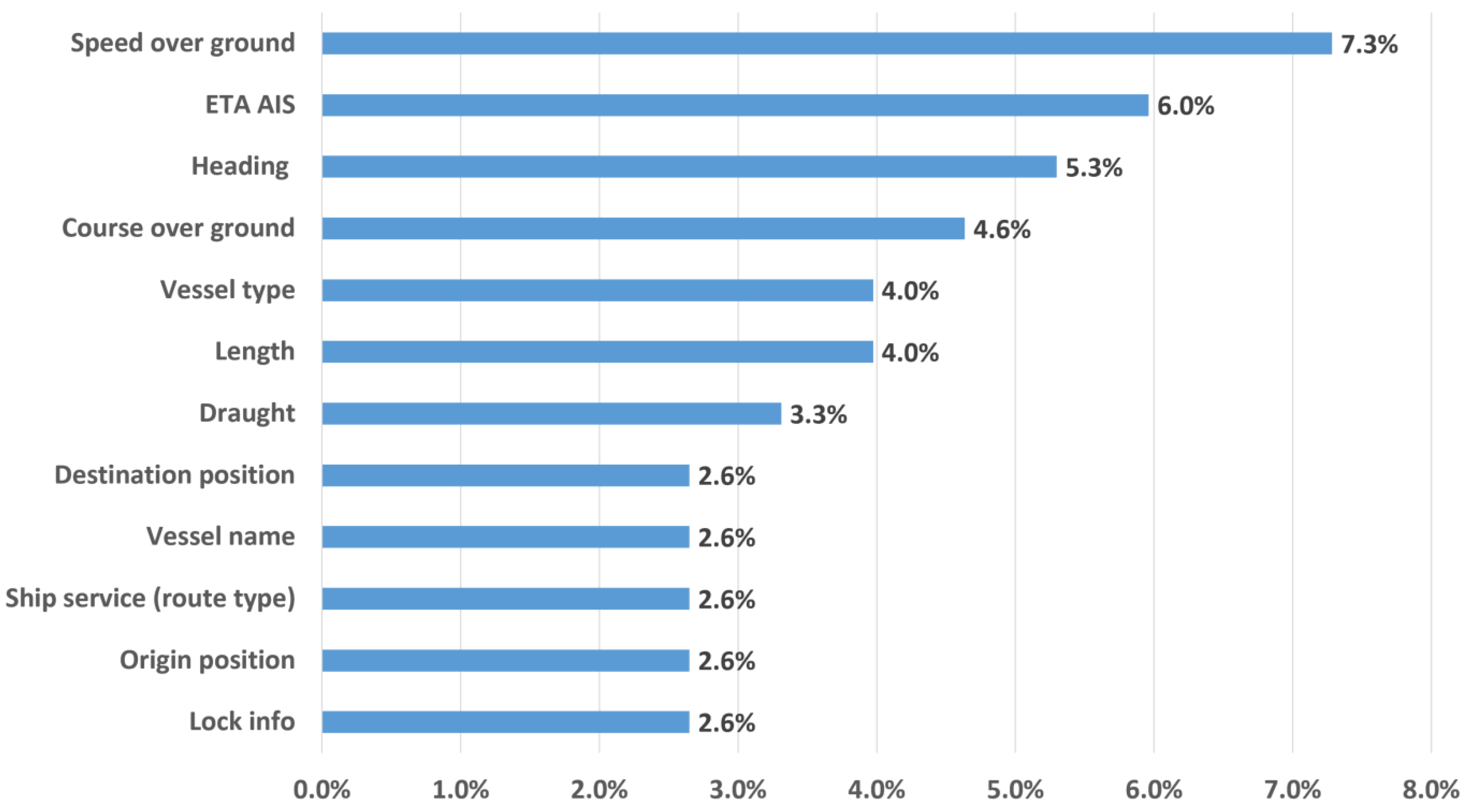
3.2. Factors Affecting ETA

Many researchers have proposed different approaches to ETA prediction, given the importance of ETA in ITSs. The performance of these methods depends on several factors, such as navigation status, weather conditions, and vessel characteristics. In order to improve the accuracy of ETA on waterway networks, it is crucial to take into account several factors, as shown in Table 2 (see column “Factors used in modeling”). Therefore, the present section aims at explaining the factors influencing the vessel navigation problems by providing descriptions of the basic terms and concepts used throughout the algorithms. El Mekkaoui et al. [16] categorized the factors used into groups, including AIS factors, vessel factors, weather factors, and craft factors. Table 1 demonstrates that there are additional factors contributing to ETA approaches that have not yet been grouped. Based on the characteristics of these factors, those with similar characteristics are included in the categories defined by El Mekkaoui et al. [16]. The remaining factors related to ship and port operations management are included in a newly introduced category called ‘operational factors’. Consequently, the factors affecting ETA can be grouped into five categories: AIS factors, vessel factors, weather factors, craft factors, and operational factors.

3.2.1. AIS Factors

AIS factors encompass a range of navigational and operational parameters tracked by AIS systems, each defined by its relevance to enhancing the precision of vessel tracking and ETA predictions.

Table 3. AISfactors contributing to ETA methods.

Factor	Description
Beam	Refers to the width of a vessel at its widest point, crucial for understanding the vessel’s size and for navigational purposes. It is often included in the literature as ‘breadth’
Course over ground (COG)	Indicates the direction in which the vessel is actually moving over the ground, which can differ from its heading due to factors like currents or wind
Draught	The vertical distance between the waterline and the bottom of the hull (keel), indicating how deep the vessel sits in the water. This determines the minimum depth of water a ship or boat can safely navigate
Heading	The direction in which the front of the vessel, or bow, is pointed, usually measured in degrees from true north.
ETA	The time when a vessel expects to arrive at a specific location, such as a port or pilot point. It is manually entered by the pilot. This is an optional field and is often not updated or reliable in raw AIS data. The ETA manually entered into the AIS systems by the pilot is also used to predict or forecast ETA using machine learning methods
Length	A key dimension, often measured from the bow to the stern. It is important for classifying the vessel size and for operational considerations in ports and harbors
MMSI	A unique nine-digit number assigned to a vessel’s AIS transponder, serving as an identification number for the vessel in radio communications
Navigational status	Indicates the operational condition of the vessel, such as whether it is underway, at anchor, moored, or not under command. It provides essential information about its current activity
Position latitude	The north–south coordinate of the vessel’s geographical position, an essential part of its global positioning for navigation and tracking
Position longitude	The east–west coordinate of the vessel’s geographical position, the second component of its precise global location
Speed over ground (SOG)	The vessel’s speed relative to the ground, which differs from the speed through water due to currents. It is important for voyage planning and safety
Timestamp	The date and time information associated with the AIS data, used to contextualize all other AIS factors in terms of when they were recorded
Vessel name	The name of the vessel as registered and displayed, used for identification and communication purposes
Vessel type	The classification of the vessel according to its purpose or physical characteristics, such as a cargo ship, tanker, or passenger ship. This is crucial for identification, regulation, and operational purposes

details the key AIS factors that influence the estimation of a vessel’s ETA.

3.2.2. Vessel Factors

Table 4. Vessel factors contributing to ETA methods.

Factors	Description
Bearing	The angle between a ship’s current position and the magnetic north
Capacity	The maximum number of containers, total volume, or weight of cargo that a vessel can carry
Deadweight tonnage (DWT)	The measure of a vessel’s carrying capacity in terms of weight, including cargo, fuel, crew, and provisions
Gross tonnage (GT)	The measure of the overall internal volume of a vessel, including all enclosed spaces
Shipping line	A company that owns and operates ships, providing information about vessel ownership, such as the owner’s name and the frequency of the vessel’s operations or voyages
Vector type	The choice between a mother vessel and a feeder vessel, considering the physical and structural differences between the two types of vessels and the different services offered by the container terminal to compensate for delays [28]
Year built	The year in which the vessel was constructed, indicating its age, which can impact its technology, efficiency, and compliance with current maritime regulations

outlines specific vessel-related factors that play crucial roles in ETA for ships. These factors encompass a range of characteristics from physical dimensions to operational capacities, which collectively influence navigational planning and logistical considerations within maritime operations.

3.2.3. Weather Factors

Various weather factors impact the accuracy of ETA predictions by influencing the movement and conditions at sea.

Table 5. Weather factors contributing to ETA methods.

Factor	Description
10 M U-component of wind	Measures the east–west component of wind speed at a height of 10 m above the sea surface, indicating the horizontal movement of air from west to east
10 M V-component of wind	Quantifies the north–south component of wind speed at 10 m above the sea surface, showing the movement of air from south to north
Humidity	The amount of water vapor present in the air, influencing comfort levels, visibility, and precipitation
Mean wave direction	The average direction from which the waves originate
Mean wave period	The average time interval between successive waves or the duration of one complete wave cycle
Meridional ocean current velocity	The speed and direction of ocean currents along the north–south axis
Significant height of combined wind waves and swell	The average height of the highest third of waves, including both wind-generated waves and swell
Significant wave height	The average height of the highest third of observed waves
Sea surface temperature	The temperature at the sea’s surface
Sea state	A description of the ocean’s surface conditions, including wave height and wind force
Water level	The depth or height of water in seas, oceans, or rivers
Temperature	The degree of hotness or coldness of the air
Wave height	The vertical distance between the crest (top) and trough (bottom) of a wave
Wind speed	The rate at which air is moving in the atmosphere
Zonal ocean current velocity	The speed and direction of ocean currents along the east–west axis

summarizes the key weather factors that contribute to ETA methods, detailing their descriptions and relevance to maritime navigation.

3.2.4. Crafted Factors

Table 6. Crafted factors contributing to ETA methods.

Factor	Description
Cumulative distance	The total moving distance from a ship’s departure to its current timestamp, often termed Destination Absolute Distance
Cumulative time	The total traveling time of a ship from departure to its current timestamp, measured in minutes
Cluster parameters	Parameters developed from route data related to the trip, such as current geofence location, last geofence location, and current country [34]
Destination position	The final point to which a vessel is traveling, critical for route planning and cargo delivery [15]
Delay	Calculated as the difference between the actual time of arrival at the pilot point and the ETA
Event time parameters	Includes parameters such as event timestamp, the exact date and time at which a specific event occurs during the vessel’s journey [11,34]. These parameters may include current day of week, current time in hours, departure day of week, and departure time in hours
Origin position	The geographical coordinates or port where a vessel begins or from which cargo originates. It could be reported as source port name [11] or trajectory origin coordinates [15,16]
Previous port distance	The distance between the previous port of call and the current or next port
Sailing status	Divided into two classes: sailed and not sailed, indicating if a vessel notified the ETA once it had left the previous port or while it was still in port
Remaining distance	The distance a ship still has to travel to reach its destination
Route leg distance	The distance between two consecutive points or stops along a vessel’s route, crucial for route planning and determining the duration of different voyage segments. A similar input feature is named absolute distance to previous [34]
Route leg speed	The average speed of a vessel over a specific leg of its journey, important for assessing the efficiency of different route segments. Similar types of route leg speed-related features, such as average speed previous, past average absolute speed, counter average speed 1 to 30, and counter average speed above 60, are considered [34]

presents the crafted factors influencing ETA methods, providing detailed descriptions in the context of efficient port operations and maritime logistics.

3.2.5. Operational Factors

Table 7. Operational factors contributing to ETA methods.

Factors	Description
Anchorage area ATA vessel	The actual time when a vessel arrives in the designated anchorage area of a port
Anchorage area ATD vessel	The actual time when a vessel departs from the anchorage area of a port
ATA at pilot point	The actual time of arrival of a vessel at the pilot point, a specific location where a harbor pilot typically boards the vessel to assist in navigating to the berth
API Call Timestamp	The exact date and time when an API call is made, commonly used in digital systems for tracking and logging data requests
Approach area ATA vessel	The actual time when a vessel arrives in the approach area of a port, typically the navigational area just before the berthing sections
Berth ATA vessel	The actual time of arrival of a vessel at its assigned berth in a port, crucial for port operations and logistics planning
Berth ATD vessel	The actual time of departure of a vessel from its berth, marking the end of its stay at that specific docking point in the port
Gateway identifier	A unique identifier used in logistics or port management systems to identify a specific entry or exit point in a terminal or port
Lock delay statistics	Measures the time spent by vessels waiting for or passing through waterway locks, providing insights into potential delays in waterway navigation and the efficiency of lock operations. Lock ATA vessel and lock ATD vessel are included in the model of Veenstra and Harmelink [35]. Pani et al. [28] considered the presence of a lock before reaching the terminal
Number of dockers required for loading/unloading	The count of dock workers needed to efficiently load or unload cargo onto a vessel
Pilot board at vessel	The moment when the navigation pilot comes aboard the vessel, typically to assist with navigating through challenging or congested waters
Pilot switch	A change or exchange of pilots on a vessel, often carried out when navigating through different territorial waters or when specialized expertise is needed
Port ATA vessel	The actual time a vessel arrives at a port
Port ETA agent	The estimated arrival time of a vessel at a port as reported by the agent
Port ETD agent	The estimated departure time from a port as reported by the agent
Ship arrival and departure declaration system from Port-MIS	A digital or electronic system used by ports to manage and track vessel arrivals and departures
Ship service variable	Represents different levels of service quality, as defined in distinct contractual agreements for different routes, including domestic trade line, trunk line, internal feeder line, and barge feeder line. Yu et al. [40] integrated domestic shipping line, and Veenstra and Harmelink [35] include first line secured at vessel and last line secured at vessel into the model
Start/End of tracking	Marks the beginning and end of the period during which a vessel’s movement is monitored or recorded
TOS Berth plan	A TOS plan that outlines the allocation of vessels to specific berths in a port
Tug standby at vessel	Refers to a tugboat being on standby near a vessel, typically for assistance with maneuvers like docking, undocking, or navigating through tight spaces
Unit load identifier	An identifier for a specific unit of cargo, used for tracking and logistics purposes

details the operational factors that significantly influence ETA predictions, elaborating on their roles within the intricacies of port operations and vessel management.

In addition, the utilization rate of factors is shown and outlined by the five primary categories AIS factors (AFs), vessel factors (VFs), weather factors (WFs), crafted factors (CFs), and operational factors (OFs). The existing literature shows that ship positional data with timestamps from AIS data sources are the main factors for ETA prediction. These three factors are the base factors, while the rest of the AFs, VFs, WFs, CFs, and OFs can be blended when modeling ETA prediction. Apart from these three base factors, the rest of the AFs are recognized as the most used factors for ETA in the existing literature (Figure 5). Figure 5 shows that the frequency of use of AFs, VFs, WFs, CFs, and OFs in ETA techniques is 43%, 7%, 15%, 14%, and 21%, respectively. Furthermore, as shown in Figure 6, SOG, manually inputted AIS ETA, heading, COG, length, vessel type, and draught are the most frequently used factors in ETA models. Moreover, AIS factors are usually combined with all other factors. A frequent combination of an AIS factor is with crafted and operational factors, both securing 33% and 33%, respectively. Additionally, researchers have combined AIS factors with vessel factors and weather factors at rates of 15% and 19%, respectively.

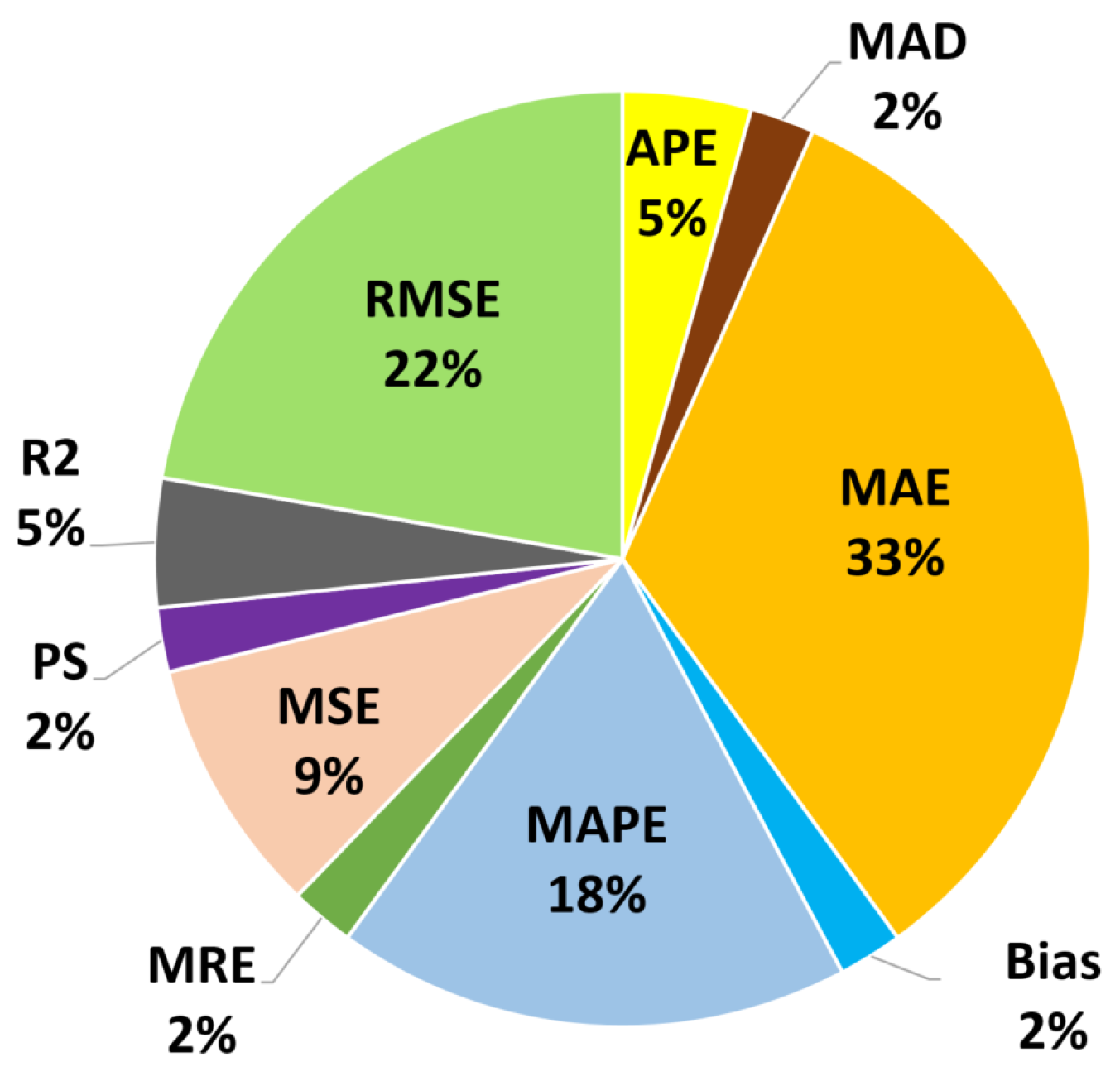
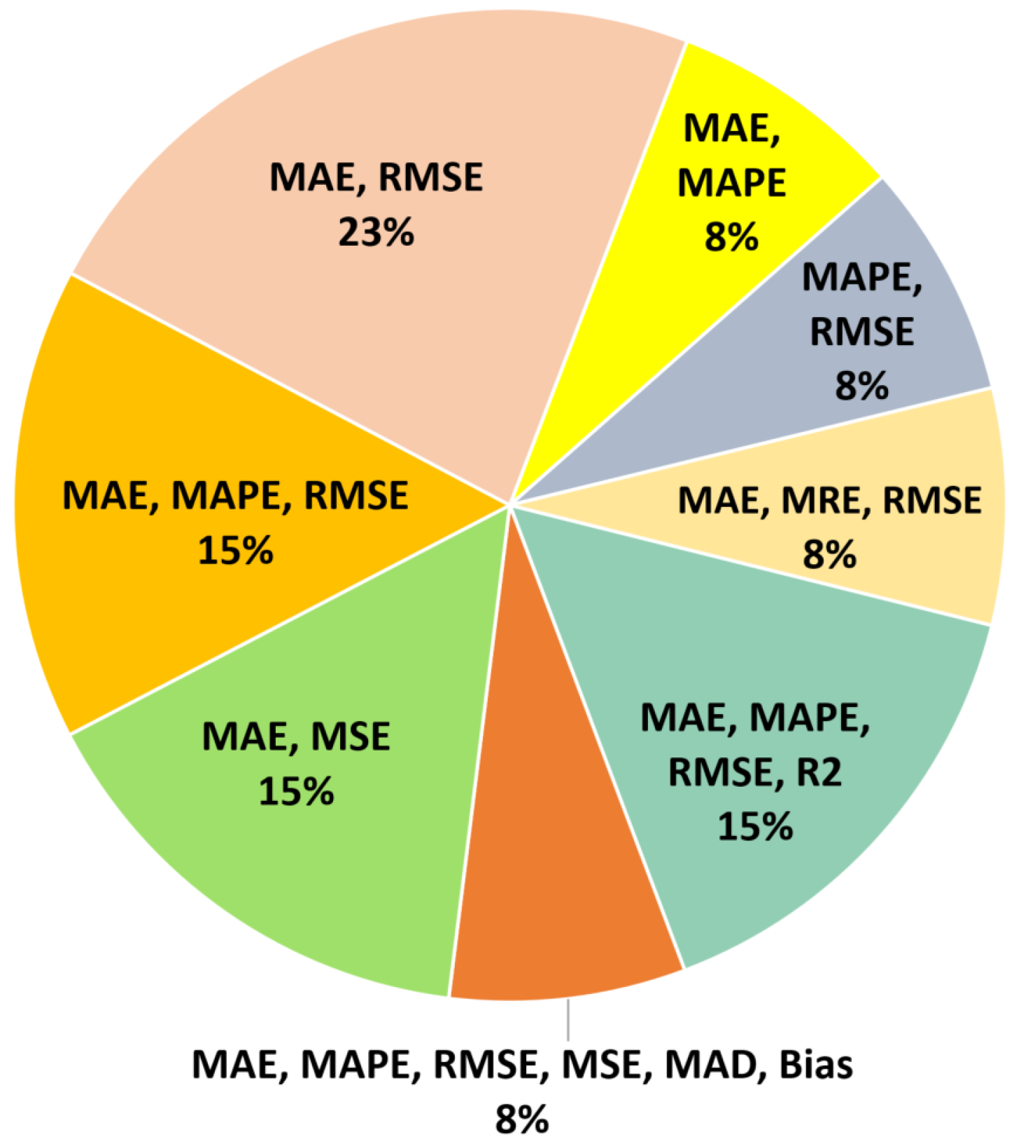
3.3. Evaluating ETA Methods

In this section, the evaluation metrics used for ETA methods are discussed. According to the literature, there are numerous approaches for estimating ETA, but determining which method performs better based on performance measures is challenging due to the diversity of datasets and domain constraints. In

Table 8. Evaluation metrics used for ETA methods.

Metric	Description
APE	This is simply the absolute value of the difference between the predicted value and the actual value. It is a measure of the accuracy of individual predictions
Bias	The error introduced when a simplified model is used to approximate a real-world problem is called bias. Underfitting occurs when an algorithm fails to recognize significant relationships between features and target outputs due to high bias
MAE	A measure of the average magnitude of errors in a set of predictions, without considering their direction. It is calculated as the average of the absolute differences between the predicted values and observed values
MSE	Similar to MAE but squares the differences before averaging them. This has the effect of giving more weight to larger errors
MAPE	Similar to MAE, but it expresses the error as a percentage of the observed values. This is particularly useful when you want to understand the relative size of the errors
RMSE	The square root of MSE. It is useful because it brings the error metric back to the same unit of measurement as the original data, making interpretation easier
MAD	Similar to MAE, it is a measure of variability that shows the average distance between each data point and the mean of the dataset
MRE	It is a statistical measure that compares the average of the absolute differences between observed and predicted values, relative to the observed values, often used to assess the accuracy of a predictive model
PS	Often used in natural language processing, perplexity is a measurement of how well a probability model predicts a sample. It is a way of evaluating language models, with lower perplexity indicating a better model
R2	A statistical measure that indicates the extent to which one or more independent variables in a regression model explain the observed variability in a dependent variable

, this literature review shows that Absolute Prediction Error (APE), bias, R-squared or Coefficient of Determination (R2), Mean Absolute Error (MAE), Mean Absolute Deviation (MAD), Root Mean Squared Error (RMSE), Mean Absolute Percentage Error (MAPE), Mean Squared Error (MSE), Perplexity Score (PS), and Mean Relative Error (MRE) are the ten evaluation metrics used in ETA predictions.

Figure 7 and Figure 8 illustrate the extent to which each metric is used, both individually and in combination (a combination of several metrics). Figure 7 illustrates the frequency of use of the metrics considered in this study: MAE (33%), RMSE (22%), MAPE (18%), MSE (5%), APE (5%), and R2 (5%). Figure 8 shows the distribution percentages of various combined metrics used in the evaluation. The analysis indicates that the most frequently employed evaluation metric combinations are as follows: MAE and RMSE (23%); MAE, MAPE, and RMSE (15%); MAE, MAPE, RMSE, and R² (15%); and MAE and MSE (15%). Therefore, the use of MAE, RMSE, and MAPE together as evaluation metrics for the ETA model allows for achieving a level of the best possible results for the methods described in the reviewed papers.

4. Open Issues

In addressing RQ3, which explores the open issues associated with ETA prediction modeling, this study shows that methodological and prediction-related issues are central obstacles in the effort to achieve accurate and reliable ETA predictions.

4.1. Method-Related Issues

Forecasting vessel ETA faces several challenges related to each category of methods for ETA prediction on waterway networks, and this section addresses those issues. Classical methods, though efficient, struggle with dynamic conditions. Shallow machine learning methods improve accuracy, but face computational issues and overfitting. Deep learning methods perform well, but require significant resources and tuning. Hybrid methods combine models to address these issues, but still encounter data uncertainties and complexity.

4.1.1. Classical Methods

Classical methods of forecasting vessel ETA, though simple and computationally efficient, face challenges in adapting to changes in waterway transportation. This inflexibility results in a limited ability to adjust to varying circumstances. These approaches are quickly implemented, contributing to their widespread practical use. Nevertheless, their accuracy tends to be compromised, primarily due to their dependence on the stability of waterway transportation in the specific region. Any changes in weather conditions or unforeseen events can greatly impede their performance. These models are reliable only if current maritime traffic closely mirrors historical traffic patterns, thus relying heavily on the regularity of waterway navigation.

4.1.2. Shallow Machine Learning Methods

In shallow machine learning methods for ETA prediction, the focus is mainly on SVM and tree-based algorithms. SVM has been particularly effective, with the choice of kernel function being critical for accuracy. The RBF kernel is commonly used due to its efficiency in mapping samples into a higher-dimensional space and its ability to handle numerical challenges more adeptly than polynomial and sigmoid kernels [34]. However, SVM is less effective with large datasets, leading to increased computational demands and storage requirements [42]. Decision trees (DTs) are popular in shallow machine learning for ETA prediction, due to advantages such as robustness to outliers and their ability to handle heavily skewed data effectively [43]. However, they are less suited for prediction tasks because of issues like overfitting and difficulties in implementing empirical risk minimization [27]. The development of ensemble methods like Gradient Boosting Decision Trees (GBDTs) has helped to mitigate some of these challenges [25]. The Random Forest (RF) model, as found by Yu et al. [40], demonstrates the best performance in predicting ship arrivals, especially when dealing with limited data [28]. This suggests the potential for improved prediction with larger datasets in future studies.

4.1.3. Deep Learning Methods

Deep learning methods, known for their flexibility, adaptability, nonlinearity, and data-driven approach, have achieved state-of-the-art performance in prediction problems. MLP, a non-sequential model, is better suited for predicting ETA for specific types of vessels, such as barges, but not universally for all types [12]. Fancello et al. [17] noted that determining the optimal hyper-parameters, like the number of hidden layers, neurons in each layer, and the activation function, is a significant challenge, often addressed through trial and error. In contrast, the study by Noman et al. [25] indicates that MLPs may not yield better results than other algorithms, such as Gated Recurrent Units (GRUs). RNNs are adept at capturing temporal correlations in data, making them suitable for time sequence processing. Enhancements like LSTM, Bidirectional LSTM (BiLSTM), and transformers have been applied to maximize the RNNs’ potential. As an illustration, El Mekkaoui et al. [14] implemented a conditional LSTM, where a dense neural network layer applies a transformation to the non-sequential data to initialise the initial hidden state. While the LSTM model is generally superior to BiLSTM and GRU in certain scenarios [41], GRU can outperform LSTM when including specific variables like waterway type [25]. Meanwhile, the BiLSTM model remains effective for merchant vessels and tugs [12]. Despite the transformer model’s capability to capture temporal events, it may be less accurate than BiLSTM or ANNs. One drawback of RNNs is the significant time required for training due to their repeated module structure in each layer, posing challenges in real-time applications. For CNN-based models, non-sequential data are transformed using a dense layer before merging with the sequential data processed by the CNN block. CNNs are widely used for extracting spatial features from datasets. Deep learning models, compared to other models, have numerous hyper-parameters, leading to high complexity and computational costs. Reducing the number of layers and hyper-parameters can be a solution to this issue. Interestingly, more complex models do not always guarantee higher accuracy. For example, the transformer model may have lower precision capabilities than simpler RNN models [12].

4.1.4. Hybrid Methods

Hybrid methods like Fuzzy Rule-Based Bayesian Networks (FRBBNs) face challenges with uncertain failure data and may not fully account for how the weight values of parameters affect the accuracy of the system’s predictions and decisions [44]. A critical limitation is their inability to consider the conditionality between interdependent factors, restricting their effectiveness in modeling complex scenarios accurately. This limitation underscores the need for ongoing improvement and adaptation of FRBBNs to enhance their effectiveness and accuracy in ETA prediction. The Kalman Filter, while optimal in scenarios with Gaussian noise, performs inadequately in the presence of non-Gaussian noise. Its reliance on a user-specified dynamic model may not accurately represent the time correlation in data. Incorporating LSTM networks could enhance accuracy, but LSTMs require extensive data for training. With limited data, LSTM performance might be compromised. This issue is particularly pertinent in complex maritime traffic conditions, where factors like weather impact ships and port congestion during peak hours, and daily time variations affect spatial correlations [41]. To address these challenges, constructing multiple models tailored to different prediction contexts could be beneficial. For instance, combining CNNs with LSTMs can capture both spatial and temporal features, offering a robust solution for varying maritime traffic conditions and enhancing prediction accuracy.

4.2. Prediction-Related Issues

This section addresses challenges and potential solutions in ETA prediction, which can involve either short-segment or long-segment forecasting. Another challenge in this field is the prediction horizon. Many studies focus on short-term predictions, using limited data that fail to capture seasonal impacts. For instance, Noman et al. [25] used only a few months of data, insufficient for assessing seasonal influences. Additionally, these studies often show reduced accuracy in long-segment predictions compared to short ones. This discrepancy might be due to the accumulation of sequence errors in predictions, leading to significant deviations in the predicted ETA. To enhance prediction accuracy, continuous revision and updating of the predicted time is one approach. Another strategy involves deploying deep machine learning models like LSTMs. LSTMs are adept at analyzing long-range dependencies, which are crucial for accuracy in long-segment or multi-segment predictions. El Mekkaoui et al. [14] demonstrated that incorporating a broader range of variables can improve prediction accuracy in specific contexts, such as ocean waterways. However, this also increases the complexity of the network. Bourzak et al. [12] showed that analyzing spatial and temporal feature vectors separately could improve model accuracy. Adding more feature vectors, such as the frequency of vessel factors and weather characteristics, might further enhance results. Most existing studies have focused on single traversal paths, overlooking interactions between different waterways. For example, Park et al. [29] and Noman et al. [25] highlight inland waterways, while El Mekkaoui et al. [14] and Jahn and Scheidweiler [20] focus on ocean routes. However, acknowledging these interactions, as indicated in these studies, can significantly improve prediction accuracy. Therefore, considering these interconnections could be crucial for developing more effective ETA prediction models.

5. Conclusions and Future Work

This paper undertakes a comprehensive literature review analysis, focusing specifically on estimated time of arrival (ETA) prediction models within the context of waterway networks. The implementation of intelligent traffic management and control systems emerges as a potential solution to address the increasing demands of supply chain logistics, reduce CO₂ emissions, enhance safety, and improve energy efficiency. The findings of this review hold the potential to guide researchers in refining and aligning their research objectives. Furthermore, this study identifies areas fit for further research, with a focus on the development of more advanced ETA prediction models. Notably, this investigation provides a comprehensive categorization of the current methodologies employed in forecasting ETA. This review reveals that ETA prediction strategies can be classified into four main categories: classical methods, shallow machine learning-based methods, deep learning-based methods, and hybrid methods. Additionally, a thorough examination of the variables that exert influence on ETA is conducted. The analysis encompasses all facets related to the model and the accuracy of ETA predictions. Based on the analysis of the selected articles, the distribution of ETA prediction techniques is as follows: classical methods account for 15%, machine learning-based methods for 42%, deep learning-based methods for 39%, and hybrid methods for 4%. In addition, a new category of factors called ’operational factors’ is introduced, and the existing categories are extended to include a wider range of factors based on their characteristics. This paper presents the utilization rates of the factors, categorized into different groups, to illustrate their application in the context of ETA prediction modeling. The distribution of factors contributing to ETA modeling is AIS factors (43%), vessel factors (7%), weather factors (15%), crafted factors (14%), and operational factors (21%). It is highlighted that common assessment metrics for ETA forecasts encompass MAE, RMSE, and MAPE.

This study has certain limitations that should be taken into account. Firstly, although the research involved a comprehensive assessment and review of a large number of papers, thereby presenting a sufficient overview of the current state of the art in the field, the conclusions drawn are limited to the chosen papers collected from several databases and review papers. This approach omits potential insights from other sources such as books, book chapters, and theses, which could also be valuable for a systematic review. Secondly, this study categorized various factors influencing ETA prediction into five groups: AIS factors, vessel factors, weather factors, crafted factors, and operational factors. However, this study did not evaluate which of these groups has the most significant impact on ETA accuracy. Furthermore, this study did not consider the sources of data, which is an aspect that should be addressed in future research to enhance the comprehensiveness and reliability of ETA predictions. To address RQ4, future research opportunities can be emphasized to overcome the limitations of current approaches and highlight notable challenges in the areas of methods, factor integration, and data anomaly handling.

5.1. Methods

Deep learning-based methods are well recognized for their robustness, ability to handle extensive datasets, capacity to uncover patterns from data, and computational efficiency. Surprisingly, relatively few proposals have been made for estimating ETA using complex deep learning methods. Therefore, it is imperative to develop prediction systems harnessing algorithms like transformers. Moreover, integrating various methodologies holds promise in enhancing and mitigating the limitations of individual approaches. Combining different approaches can offer a versatile strategy to address unforeseen circumstances, potentially benefiting ETA prediction. For instance, Zhang et al. [41] propose the fusion of the Kalman Filter with Long Short-Term Memory (LSTM) for ETA forecasting. Due to the large amount of transportation data that can be collected, which include sequential and non-sequential data, combining deep learning algorithms that can handle both data types could be beneficial. However, developing such hybrid models requires a comprehensive understanding of the properties of existing approaches, guiding the research direction of Section 5.2 and Section 5.3.

5.2. Integrating Factors

One significant drawback of the current systems is their limited accuracy in responding to changes induced by unforeseen events. Future research should prioritize the rapid identification of unforeseen occurrences to adapt to unexpected navigation scenarios. Most reviewed articles relied on a single type of waterway AIS data as input for their models, with only a few incorporating additional types of waterway data. A single dataset may not adequately capture the complexity of waterway transit scenarios. Therefore, integrating various types of waterway data could enhance the precision of ETA prediction techniques. Additionally, many existing approaches have overlooked the impact of lock delays and climate change factors. Since ETA is subject to fluctuations in both time and location, an approach that accounts for spatial and temporal variations can offer a more accurate picture of traffic conditions, ultimately reducing ETA uncertainty. Future endeavors should involve the incorporation of all potential factors, analyzed to enhance predictive operations. However, not all factors from a comprehensive list may be suitable for distinct waterways. Therefore, future research should also focus on investigating these factors and compiling a list of important factors from each category that could impact ETA modeling.

5.3. Handling Data Anomalies

When considering large amounts of data, it is essential to recognize that while AIS data are generally accurate, they are not immune to anomalies [45]. To develop a robust ETA prediction model, it is imperative to account for these data anomalies in future research endeavors.

References

1. UNCTAD. Review of Maritime Transport 2017; UNCTAD: Geneva, Switzerland, 2017. [Google Scholar]
2. Dobrkovic, A.; Liu, L.; Iacob, M.E.; van Hillegersberg, J. Intelligence amplification framework for enhancing scheduling processes. In Proceedings of the Advances in Artificial Intelligence-IBERAMIA, San Jose, Costa Rica, 23–25 November 2016; pp. 89–100. [Google Scholar] [CrossRef]
3. Salido, M.A.; Rodriguez-Molins, M.; Barber, F. A decision support system for managing combinatorial problems in container terminals. Knowl.-Based Syst. 2012, 29, 63–74. [Google Scholar] [CrossRef]
4. Rocha de Paula, M.; Boland, N.; Ernst, A.T.; Mendes, A.; Savelsbergh, M. Throughput optimisation in a coal export system with multiple terminals and shared resources. Comput. Ind. Eng. 2019, 134, 37–51. [Google Scholar] [CrossRef]
5. Li, J.; Zhang, X.; Yang, B.; Wang, N. Vessel traffic scheduling optimization for restricted channel in ports. Comput. Ind. Eng. 2021, 152, 107014. [Google Scholar] [CrossRef]
6. Kitchenham, B.; Charters, S. Guidelines for Performing Systematic Literature Reviews in Software Engineering; Technical Report EBSE 2007-001. Keele University and Durham University Joint Report; UK, 2007. Available online: https://edisciplinas.usp.br/pluginfile.php/4108896/mod_resource/content/2/slrPCS5012_highlighted.pdf (accessed on 2 June 2024).
7. Snyder, H. Literature review as a research methodology: An overview and guidelines. J. Bus. Res. 2019, 104, 333–339. [Google Scholar] [CrossRef]
8. Page, M.J.; McKenzie, J.E.; Bossuyt, P.M.; Boutron, I.; Hoffmann, T.C.; Mulrow, C.D.; Shamseer, L.; Tetzlaff, J.M.; Akl, E.A.; Brennan, S.E.; et al. The PRISMA 2020 statement: An updated guideline for reporting systematic reviews. BMJ 2021, 372, n71. [Google Scholar] [CrossRef] [PubMed]
9. Alessandrini, A.; Mazzarella, F.; Vespe, M. Estimated time of arrival using historical vessel tracking data. IEEE Trans. Intell. Transp. Syst. 2019, 20, 7–15. [Google Scholar] [CrossRef]
10. Bodunov, O.; Schmidt, F.; Martin, A.; Brito, A.; Fetzer, C. Real-time destination and ETA prediction for maritime traffic. In Proceedings of the DEBS 2018—12th ACM International Conference on Distributed and Event-Based Systems, Hamilton, New Zealand, 25–29 June 2018. [Google Scholar] [CrossRef]
11. Bachar, M.; Elimelech, G.; Gat, I.; Sobol, G.; Rivetti, N.; Gal, A. Venilia, Online learning and prediction of vessel destination. In Proceedings of the DEBS 2018—12th ACM International Conference on Distributed and Event-Based Systems, Hamilton, New Zealand, 25–29 June 2018. [Google Scholar] [CrossRef]
12. Bourzak, I.; Mekkaoui, S.E.; Berrado, A.; Caron, S.; Benabbou, L. Deep learning approaches for vessel estimated time of arrival prediction: A case study on the Saint Lawrence river. In Proceedings of the 2023 14th International Conference on Intelligent Systems: Theories and Applications (SITA), Casablanca, Morocco, 22–23 November 2023. [Google Scholar] [CrossRef]
13. Chu, Z.; Yan, R.; Wang, S. Evaluation and prediction of punctuality of vessel arrival at port: A case study of Hong Kong. Marit. Policy Manag. 2024, 51, 1096–1124. [Google Scholar] [CrossRef]
14. Mekkaoui, S.E.; Benabbou, L.; Berrado, A. Predicting ships estimated time of arrival based on AIS data. In Proceedings of the SITA’20: Proceedings of the 13th International Conference on Intelligent Systems: Theories and Applications, Rabat, Morocco, 23–24 September 2020. [CrossRef]
15. Mekkaoui, S.E.; Benabbou, L.; Berrado, A. Machine learning models for efficient port terminal operations: Case of vessels’ arrival times prediction. IFAC-PapersOnLine 2022, 55, 3172–3177. [Google Scholar] [CrossRef]
16. Mekkaoui, S.E.; Benabbou, L.; Berrado, A. Deep learning models for vessel’s ETA prediction: Bulk ports perspective. Flex. Serv. Manuf. J. 2023, 35, 5–28. [Google Scholar] [CrossRef]
17. Fancello, G.; Pani, C.; Pisano, M.; Serra, P.; Zuddas, P.; Fadda, P. Prediction of arrival times and human resources allocation for container terminal. Marit. Econ. Logist. 2011, 13, 142–173. [Google Scholar] [CrossRef]
18. Fan, T.; Chen, D.; Huang, C.; Tian, C.; Yan, X. Inland vessel travel time prediction via a context-aware deep learning model. J. Mar. Sci. Eng. 2023, 11, 1146. [Google Scholar] [CrossRef]
19. Huang, C.; Huang, Y.; Yu, Y.; Xiao, B. Predicting liner arrival time based on deep learning. In Proceedings of the 2021 IEEE 3rd International Conference on Civil Aviation Safety and Information Technology, ICCASIT 2021, Changsha, China, 20–22 October 2021. [Google Scholar] [CrossRef]
20. Jahn, C.; Scheidweiler, T. Port Call Optimization by Estimating Ships’ Time of Arrival; Springer: Berlin/Heidelberg, Germany, 2018. [Google Scholar] [CrossRef]
21. Kolley, L.; Rückert, N.; Kastner, M.; Jahn, C.; Fischer, K. Robust berth scheduling using machine learning for vessel arrival time prediction. Flex. Serv. Manuf. J. 2023, 35, 29–69. [Google Scholar] [CrossRef]
22. Kwun, H.; Bae, H. Prediction of vessel arrival time usingc auto identification system data. Int. J. Innov. Comput. Inf. Control. 2021, 17, 725–734. [Google Scholar] [CrossRef]
23. Lin, C.X.; Huang, T.W.; Guo, G.; Wong, M.D.F. MtDetector: A high-performance marine traffic detector at stream scale. In Proceedings of the 12th ACM International Conference on Distributed and Event-Based Systems, Hamilton, New Zealand, 25–29 June 2018; pp. 205–208. [Google Scholar] [CrossRef]
24. Nguyen, D.D.; Van, C.L.; Ali, M.I. Vessel trajectory prediction using sequence-to-sequence models over spatial grid. In Proceedings of the DEBS 2018—12th ACM International Conference on Distributed and Event-Based Systems, Hamilton, New Zealand, 25–29 June 2018. [Google Scholar] [CrossRef]
25. Noman, A.A.; Heuermann, A.; Wiesner, S.A.; Thoben, K.D. Towards data-driven GRU based ETA prediction approach for vessels on both inland natural and artificial waterways. In Proceedings of the IEEE Conference on Intelligent Transportation Systems, Proceedings, ITSC, , Indianapolis, IN, USA, 19–22 September 2021; Volume 2021. [Google Scholar] [CrossRef]
26. Ogura, T.; Inoue, T.; Uchihira, N. Prediction of arrival time of vessels considering future weather conditions. Appl. Sci. 2021, 11, 4410. [Google Scholar] [CrossRef]
27. Pani, C.; Fadda, P.; Fancello, G.; Frigau, L.; Mola, F. A data mining approach to forecast late arrivals in a transhipment container terminal. Transport 2014, 29, 175–184. [Google Scholar] [CrossRef]
28. Pani, C.; Vanelslander, T.; Fancello, G.; Cannas, M. Prediction of late/early arrivals in container terminals—A qualitative approach. Eur. J. Transp. Infrastruct. Res. 2015, 15, 536–550. [Google Scholar] [CrossRef]
29. Park, K.; Sim, S.; Bae, H. Vessel estimated time of arrival prediction system based on a Path-Finding algorithm. Marit. Transp. Res. 2021, 2, 100012. [Google Scholar] [CrossRef]
30. Rahman, M.; Haque, E.; Tasneem Rahman, S.; Ahmed, Y.; Habibul Kabir, K. Modelling of an efficient system for prediction ships’ estimated time of arrival using artificial neural network. In Computational Intelligence; Lecture Notes in Electrical Engineering; Shukla, A., Murthy, B., Hasteer, N., Van Belle, J.P., Eds.; Springer: Berlin/Heidelberg, Germany, 2023; Volume 968, pp. 199–206. [Google Scholar] [CrossRef]
31. Roşca, V.; Diac, P.; Onica, E.; Amariei, C. Predicting destinations by Nearest Neighbor Search on training vessel routes. In Proceedings of the DEBS 2018—12th ACM International Conference on Distributed and Event-Based Systems, Hamilton, New Zealand, 25–29 June 2018. [Google Scholar] [CrossRef]
32. Salleh, N.H.M.; Riahi, R.; Yang, Z.; Wang, J. Predicting a containership’s arrival punctuality in liner operations by Using a Fuzzy Rule-based Bayesian Network (FRBBN). Asian J. Shipp. Logist. 2017, 33, 95–104. [Google Scholar] [CrossRef]
33. Sathiaraj, D.; Smith, A.; Rohli, E.; Hsieh, C.; Salindong, A.; Woolsey, N.; Tec, A. RippleGo—An AI-based voyage planner for US inland waterways. In Proceedings of the 2023 IEEE Conference on Artificial Intelligence, CAI 2023, Santa Clara, CA, USA, 5–6 June 2023. [Google Scholar] [CrossRef]
34. Servos, N.; Liu, X.; Teucke, M.; Freitag, M. Travel time prediction in a multimodal freight transport relation using machine learning algorithms. Logistics 2020, 4, 1. [Google Scholar] [CrossRef]
35. Veenstra, A.W.; Harmelink, R.L. Process mining ship arrivals in port: The case of the port of Antwerp. Marit. Econ. Logist. 2022, 24, 584–601. [Google Scholar] [CrossRef]
36. Jung, H.; Lee, K.W.; Choi, J.H.; Cho, E.S. Bayesian estimation of vessel destination and arrival times. In Proceedings of the DEBS ’18: 12th ACM International Conference on Distributed and Event-Based Systems, Hamilton, New Zealand, 25–29 June 2018. [Google Scholar] [CrossRef]
37. Wenzel, P.; Jovanovic, R.; Schulte, F. A Neural Network approach for ETA prediction in inland waterway transport. Lect. Notes Comput. Sci. 2023, 14239, 219–232. [Google Scholar] [CrossRef]
38. Wu, X.; Roy, U.; Hamidi, M.; Craig, B.N. Estimate travel time of ships in narrow channel based on AIS data. Ocean. Eng. 2020, 202, 106790. [Google Scholar] [CrossRef]
39. Yoon, J.H.; Kim, D.H.; Yun, S.W.; Kim, H.J.; Kim, S. Enhancing vontainer vessel arrival time prediction through past voyage route modeling: A case study of Busan new port. J. Mar. Sci. Eng. 2023, 11, 1234. [Google Scholar] [CrossRef]
40. Yu, J.; Tang, G.; Song, X.; Yu, X.; Qi, Y.; Li, D.; Zhang, Y. Ship arrival prediction and its value on daily container terminal operation. Ocean. Eng. 2018, 157, 73–86. [Google Scholar] [CrossRef]
41. Zhang, X.; Zhang, X.; Li, P. Prediction model of ship arrival time using Neural Network and Kalman Filter. In Proceedings of the 2023 3rd International Conference on Neural Networks, Information and Communication Engineering, NNICE 2023, Guangzhou, China, 24–26 February 2023. [Google Scholar] [CrossRef]
42. Awad, M.; Khanna, R. Support Vector Machines for classification. In Efficient Learning Machines: Theories, Concepts, and Applications for Engineers and System Designers; Apress: Berkeley, CA, USA, 2015. [Google Scholar] [CrossRef]
43. Song, Y.Y.; Lu, Y. Decision tree methods: Applications for classification and prediction. Shanghai Arch. Psychiatry 2015, 27, 130–135. [Google Scholar] [CrossRef] [PubMed]
44. Yucesan, M.; Gul, M.; Celik, E. A holistic FMEA approach by Fuzzy-based Bayesian Network and best–worst method. Complex Intell. Syst. 2021, 7, 1547–1564. [Google Scholar] [CrossRef]
45. Yang, D.; Wu, L.; Wang, S.; Jia, H.; Li, K.X. How big data enriches maritime research – a critical review of Automatic Identification System (AIS) data applications. Transp. Rev. 2019, 39, 755–773. [Google Scholar] [CrossRef]
Figure 1. Map of a North Sea waterway and inland waterways, including both artificial and natural routes.
Computers 14 00041 g001
Figure 2. Overview of the review process.
Computers 14 00041 g002
Figure 3. Most-used category of ETA methods.
Computers 14 00041 g003
Figure 4. Most-used algorithms with percentage.
Computers 14 00041 g004
Figure 5. Distribution of factors used in ETA methods.
Computers 14 00041 g005
Figure 6. Most commonly used factors for ETA methods.
Computers 14 00041 g006
Figure 7. Most commonly used evaluation metrics for ETA estimation.
Computers 14 00041 g007
Figure 8. Distribution of combined evaluation metrics for ETA estimation.
Computers 14 00041 g008