A Multi-Step PM2.5 Time Series Forecasting Approach for Mining Areas Using Last Day Observed, Correlation-Based Retrieval, and Interpolation

Abstract

Monitoring PM2.5 in mining areas is essential for air quality management; however, most studies focus on single-step forecasts, limiting timely decision making. This work addresses the need for accurate multi-step PM2.5 prediction to support proactive pollution control in mining regions. So, a new model for multi-step PM2.5 time series forecasting is proposed, which is based on historical data such as the last day observed (LDO), retrieved data by correlation levels, and linear interpolation. As case studies, data from three environmental monitoring stations in mining areas of Peru were considered: Tala station near the Cuajone mine, Uchumayo near the Cerro Verde mine, and Espinar near the Tintaya mine. The proposed model was compared with benchmark models, including Long Short-Term Memory (LSTM), Bidirectional LSTM (BiLSTM), Gated Recurrent Unit (GRU), and Bidirectional GRU (BiGRU). The results show that the proposed model achieves results similar to those obtained by the benchmark models. The main advantages of the proposed model over the benchmark models lie in the amount of data required for predictions and the training time, which represents less than 0.2% of that required by deep learning-based models.

1. Introduction

Fine particulate matter (PM2.5) is one of the most dangerous forms of air pollution [1,2], as its particles have a diameter of less than 2.5 μm [3], allowing them to penetrate deep into the lungs [4] and reach the bloodstream [5], which can cause serious short- and long-term health problems.

One of Peru’s main economic activities is mining [6]. In this study, three regions with significant mining activity were selected: Moquegua, Arequipa, and Cusco, where the Environmental Assessment and Enforcement Organization (OEFA) of the Ministry of the Environment (Peru) has implemented PM10 and PM2.5 monitoring stations.

This study focuses on PM2.5, which consists of fine dust generated by rock blasting, mineral transportation, and crushing processes. PM2.5 can cause various respiratory issues and lung diseases. Thus, PM2.5 levels are analyzed in three mining regions of Peru—Moquegua, Arequipa, and Cusco—where copper is the primary mineral produced. In Moquegua, data from the Tala station near the Cuajone mine [7] was used; in Arequipa, data from the Uchumayo station near the Cerro Verde mine was used [8]; and in Cusco, data from the Espinar station near the Tintaya mine was used [9].

According to the literature review, most studies related to air pollutants are focused on those generated by industrial activity, while a smaller number of studies are focused on mining activity. In mining areas, the most common air pollutants [10] include particulate matter (PM10 and PM2.5), sulfur dioxide (SO₂) [11], nitrogen oxides (NO_x) [12], carbon monoxide (CO), heavy metals (lead, mercury, arsenic, and cadmium) [13], and volatile organic compounds. These pollutants affect air quality, the health of nearby communities, and ecosystems.

Likewise, a large number of related works are focused on single-step PM2.5 forecasting; however, for timely decision making regarding this type of atmospheric pollutant, multi-step PM2.5 forecasts are required, and in many cases, air quality management decisions must be taken more than 10 h ahead of time [14].

In this work, a new model is proposed for multi-step PM2.5 time series forecasting based on the last day observed, correlation days, and linear interpolation. The last observed day component is inspired by the Last Observed Carried Forward (LOCF) imputation technique [15], which allows for obtaining results similar to the observed data. For the correlation days, the average of the two days with the highest correlation in the training data is calculated; unlike similar techniques, not all the training data are considered but only a smaller subset that meets the required minimum correlation level. Finally, linear interpolation is applied to smooth the results obtained by the previous techniques and better approximate the estimates to the observed data. The results obtained are compared with well-known state-of-the-art models such as LSTM, BiLSTM, GRU, and BiGRU.

The main contributions of this work are listed below:

−

A new model for multi-step, hourly PM2.5 time series forecasting.

−

A comparative study between the proposed model and benchmark models for PM2.5 forecasting in mining areas of Peru.

2. Literature Review

2.1. Overview of Forecasting Models

Forecasting models for time series have evolved from statistical to machine learning and deep learning models. Among the statistical models, one of the best known is ARIMA [16] and its variants, while another widely used model is Multiple Linear Regression (MLR); however, these models often fail to capture nonlinear relationships and temporal dependencies. Machine learning-based models include Support Vector Regression (SVR) [17], K-Nearest Neighbors [18], and ensemble models such as gradient boosting [19], random forests [20], and AdaBoost [21], among others. Recently, deep learning models such as those based on recurrent neural networks include LSTM, GRU, BiLSTM, BiGRU, and LSTM with attention layers. Finally, those based on Transformers [22,23,24] are gaining popularity. Deep learning models, unlike the former, require large amounts of data and have a high computational cost for training.

2.2. One-Step-Related Works

Based on the literature review, most related studies have proposed and implemented LSTM-based models. Among them, Refs. [19,25,26,27,28,29,30] stand out, with some incorporating decomposition techniques and others combining LSTM with additional approaches. For instance, ref. [27] introduced a decomposition method known as Singular Spectrum Analysis (SSA). In [25,26], Bidirectional LSTM (BiLSTM) and standard LSTM were employed, respectively. The study in [28] combined LSTM with Convolutional Neural Networks (CNNs), while ref. [30] integrated a Bidirectional LSTM with a CNN architecture. Additionally, ref. [29] implemented LSTM along with decomposition techniques such as CEEMDAN and FCM. Furthermore, GRU models were explored in [31,32], combined with data augmentation and Q-Learning, respectively.

Another group of studies use machine learning techniques, such as Support Vector Regression (SVR) and random forest. Random forest was used in [33], SVR with Quantum Particle Swarm Optimization (QPSO) was used in [34], and SVR with a decomposition technique named hybrid modified variational mode decomposition was used in [35].

Also, some related works, including [36,37,38,39,40], implemented different approaches to those cited before. In [36], a Hammerstein recurrent neural network was proposed; in [25], the authors propose decomposition ensemble learning based on variation mode decomposition and the whale-optimization algorithm (IWOA); the authors of [39] propose an attention-based deep neural network; ref. [40] proposes a multivariate deep belief network using PM2.5 and temperature data; and in [37], a Multiple Model Adaptive Unscented Kalman Filter is proposed.

2.3. Multi-Step-Related Works

In [41,42], the authors proposed the use of Extreme Learning Machine (ELM), achieving MAPEs ranging from 5.11% to 37.23% for three-step forecasting, and from 5.12% to 22.2% for seven-step forecasting. In [43], a hybrid CNN-LSTM architecture was applied for 10-step forecasting, yielding MAPEs between 22.09% and 25.94%. The study in [44] implemented the AdaBoost algorithm, obtaining MAPEs between 15.32% and 23.75% for three-step predictions. In [45], Support Vector Machine (SVM) was utilized for four-step forecasting, reporting RMSE values between 8.16 and 39.04 μg/m³. In [46], a Self-Organizing Memory Neural Network was employed for 1-, 4-, 8-, and 12-day forecasts, achieving MAPEs between 6.66% and 14.08%. The work in [47] incorporated a genetic algorithm-based feature selection approach to optimize an LSTM model for one- to six-step forecasting, obtaining MAEs ranging from 3.592 to 6.684. In [48], a BiLSTM model was applied for three-step forecasting, achieving MAPEs between 27.33% and 40.73%. Studies [49,50] proposed CNN-based models for 10-step and 4-step forecasting, obtaining MAPEs between 28.51% and 33.29%. Study [51] introduced a point-based system for three-step forecasting, resulting in MAPEs between 7.53% and 16.18%. In [52], a statistical approach for multi-step forecasting was proposed, combining weighted averages and polynomial interpolation. In [53] a graph convolutional network with an attention mechanism was proposed for one-, two-, and three-step forecasting, resulting in RMSEs between 4.21 and 6.54 ug/m³.

Table 1. Multi-step-related works for PM2.5 forecasting.

Work	Technique	Steps	Metric	Results	Description
[41,42]	Extreme Learning Machine (ELM)	3 steps, 7 steps	MAPE	5.11–37.23% (3 steps); 5.12–22.2% (7 steps)	Demonstrated ELM capability for short- and mid-term PM2.5 forecasting.
[43]	Hybrid CNN–LSTM	10 steps	MAPE	22.09–25.94%	Combined spatial and temporal feature extraction for extended forecasts.
[44]	AdaBoost	3 steps	MAPE	15.32–23.75%	Ensemble learning improved short-term prediction accuracy.
[45]	Support Vector Machine (SVM)	4 steps	RMSE (μg/m3)	8.16–39.04	Showed nonlinear regression performance of SVM for PM2.5 estimation.
[46]	Self-Organizing Memory Neural Network	1, 4, 8, and 12 steps	MAPE	6.66–14.08%	Captured temporal dependencies over multiple horizons.
[47]	LSTM + genetic algorithm (feature selection)	1–6 steps	MAE	3.592–6.684	Optimized feature selection improved LSTM predictive performance.
[48]	BiLSTM	3 steps	MAPE	27.33–40.73%	Evaluated bidirectional memory for temporal dependency modeling.
[48,49]	CNN-based models	10 steps, 4 steps	MAPE	28.51–33.29%	Highlighted the potential of convolutional structures in PM2.5 prediction.
[51]	Point-based system	3 steps	MAPE	7.53–16.18%	Proposed point-wise modeling for improved local forecasting.
[52]	Weighted average + polynomial interpolation	24 steps	MAPE	17.69 –28.91%.	Introduced a statistical hybrid method for multi-step forecasting.
[53]	Graph convolutional network (GCN) + attention mechanism	1, 2, 3 steps	RMSE	4.21–6.54 (μg/m3)	Modeled spatial–temporal dependencies using graph-based architecture.

shows a summary of these works.

Based on the reviewed works in this stage, most single- and multi-step PM2.5 forecasting studies have focused on machine learning and deep learning approaches, including hybrid architectures, decomposition methods, and data augmentation strategies. The majority of these works address single-step or short-term forecasting. However, as noted in [14], air quality decisions often need to be made more than 10 h in advance, while the maximum forecast horizon commonly reported in the literature is 10 steps (10 h). This was the main motivation for conducting this study, which implements a model for 24 steps ahead. The main differences between the proposed model and related works are shown in

Table 2. Main differences between proposal model and related works.

Related Works	Proposal Model
Most of them are based on machine and deep learning.	The proposal is based on correlations and interpolation.
Most of them were implemented for one-step forecasting.	This study was implemented for multi-step forecasting.
Machine and deep learning models require a lot of training data.	The proposed model requires fewer training data.
Most existing studies were implemented for air pollutants generated by industrial activity.	This study is proposed for air pollutants generated by mining activity.

.

3. Materials and Methods

3.1. Data Collection

The hourly data used for this work were downloaded from the OEFA’s server located at https://pifa.oefa.gob.pe/VigilanciaAmbiental/, accessed on 30 August 2025, and they correspond to three environmental monitoring stations (Tala, Uchumayo, and Espinar) located in Peru. Figure 1 shows the locations of the three monitoring stations.

3.2. Data Preparation

The data organized in a one-dimensional array were restructured into a two-dimensional array, that is, in matrix form, where each row of the matrix contains 24 columns corresponding to the hours of a day.

The collected data contained several missing values; therefore, all days with incomplete records were removed from the dataset. Following this preprocessing step, the total number of available records for each monitoring station was summarized (

Table 3. Data of environmental monitoring stations.

Station	Total Hours	Training: 80%	Testing: 20%
Tala	15,936 (664 days)	12,744 (531 days)	3192 (133 days)
Uchumayo	6312 (263 days)	5040 (210 days)	1272 (53 days)
Espinar	20,232 (843 days)	16,176 (674 days)	4056 (169 days)

). Additionally, since the study addresses a regression problem, and in accordance with recommendations from the statistical modeling literature, the dataset was divided into two subsets: 80% for training and 20% for testing.

3.3. The Proposed Model

3.3.1. Last Day Observed (LDO)

As observed in multiple imputation studies and in some time series forecasting works, the last observed values show a high correlation with the values to be estimated. In this study, for the proposed model, the first phase used the data from the last observed day (LDO). Thus, applying this approach to the first day of the test data at the Uchumayo station yielded the results shown in Figure 2.

3.3.2. Retrieving by Correlation

In this phase, the two days with the highest correlation are searched within the training data. However, the search is not performed across the entire dataset, but only within a limited number of days, since it is assumed that the data closer to the day to be predicted are the most similar. For this study, it was determined that for the Uchumayo station, using 30 days satisfied the condition of a minimum correlation level > 0.2. For the Tala and Espinar stations, the required number was 20 days.

Once the optimal number of days is determined, the two days with the highest correlation are retrieved and averaged. Figure 3 shows the result of this operation for 1 day (equivalent to 24 h) at the Uchumayo station.

Table 4. Average retrieved days for correlation levels.

Correlation Level	Dataset
	Tala	Uchumayo	Espinar
0.1	13.6	17.6	15.5
0.2	11.1	14.5	13.7
0.3	*	*	*
0.4	*	*	*

* There are days to predict that do not retrieve data for the correlation level.

shows the average retrieved days for different correlation levels.

According to Table 4, it can be seen that for the datasets, to ensure that the search return results complete the predictions of the test data, it is necessary to set a correlation level of 0.2; for higher values, it is not guaranteed that predictions can be completed for all the test data.

3.3.3. Averaging LDO and Retrieved Data

Observing Figure 3, it can be seen that in the previous stages, the predicted data are found both above and below the observed values; therefore, averaging them can better approximate the results to the observed data. Figure 4 presents the results.

3.3.4. Applying Linear Interpolation

Once the 24 h prediction has been obtained, as the average of the days with the highest correlation, linear interpolation is applied. For this purpose, Equation (1) is used:

$$y={\displaystyle \frac{y_1-y_0}{x_1-x_0}}\left(x-x_0\right)+y_0$$

(1)

where y is the value to be estimated from a pair of points.

As shown in Figure 5, linear interpolation smooths the predicted curve from the previous phase. Although in this example it does not improve the prediction, in most cases it does, as presented in Section 4.

It is important to highlight that the number of elements to interpolate is different for each monitoring station; that is, experiments were conducted with varying amounts, from 1 to 7 items, resulting in the optimal values of 6, 5, and 5 for the Tala, Uchumayo, and Espinar stations, respectively.

The logic used to estimate the mean of the retrieved data is implemented in Algorithm 1.

Algorithm 1. Function to retrieve day(s) with best correlation(s)
1	function predict(trn, row, hrows)
2	ntrn = len(trn)
3	row1 = []
4	row2 = []
5	max1 = 0
6	max2 = 0
7	i = ntrn-2
8	while i > = 0
9	corr = pearson(row, trn [i])
10	if max1 < corr
11	row2 = row1 #the predicted day2
12	row1 = trn [i + 1] #the predicted day1
13	max2 = max1
14	max1 = corr
15	i = i-1
16	min_level = 0.20
17	mrow = []
18	if max1 > min_level and max2 > min_level
19	mrow = (row1 + row2)/2
20	if max1 > min_level and max2 < = min_level
21	mrow = row1
22	if max1 < = min_level and max2 > min_level
23	mrow = row2
24	return(mrow)

The algorithm for retrieving the days with the highest correlation receives the parameters trn, row, and hrows. trn represents the training data matrix, row is the last day observed (LDO), and hrows is the number of days to consider for the search within the trn matrix. Between lines 2 and 6, the variables required by the algorithm are initialized. Between lines 7 and 15, the search for the most correlated days is carried out using the Pearson correlation. Finally, between lines 16 and 24, it is verified whether the correlation levels exceed the minimum required threshold, returning either the average or the row with the highest correlation.

The function that averages the LDO with the retrieved data is shown in Algorithm 2. It receives as parameters the training and testing data in trn and tst, as well as the number of historical days to consider for the search. Between lines 2 and 6, the variables required by the algorithm are initialized. Between lines 7 and 11, the average between the LDO and the retrieved data obtained with Algorithm 1 is calculated. Finally, between lines 12 and 15, the respective average for the last day of the test data is estimated, and the predicted values are returned.

Algorithm 2. Function to average LDO and retrieved data
1	function average(trn, tst, hrows)
2	hrows = 30 #depends on the dataset used
3	last = len(trn)-1
4	ntst = len(tst)
5	row = trn [last]
6	preds = []
7	for j = 0->ntst-1
8	mrow = predict(trn, row, hrows)
9	r_ldo = (row + mrow)/2
10	row = tst [j]
11	preds.append(r_ldo)
12	mrow = predict (trn, row, hrows)
13	r_ldo = ((np.array(row) + np.array(mrow))/2)
14	preds.append(r_ldo)
15	return(preds)

3.4. Evaluation

The achieved results are evaluated using three metrics, which include the Root-Mean-Squared Error (RMSE), which allows for assessing the prediction error in terms of the original values of the time series; the Mean Absolute Percentage Error (MAPE), which evaluates the results in percentage terms; and finally, the correlation coefficient (R), which measures the level of correlation between the observed and predicted data. Equations (2)–(4) enable their implementation:

$$RMSE=\sqrt{{\displaystyle \frac{\sum _{i=1}^n{\left(P_i-O_i\right)}^2}{n}}}$$

(2)

$$MAPE={\displaystyle \frac{1}{n}}{\sum }_{i=1}^n\left|{\displaystyle \frac{\left(O_i-P_i\right)}{O_i}}\ast 100\right|$$

(3)

$$R=\sqrt{{\displaystyle \frac{ \sum _{i=1}^n(P_i-\overline{P})(O_i-\overline{O})}{\sum _{i=1}^n{\left(P_i-\overline{P}\right)}^2\sum _{i=1}^n{\left(O_i-\overline{O}\right)}^2}}}$$

(4)

where $P_i$ is each predicted value, $O_i$ is each observed value, n is the total number of predicted data points, $\overline{P}$ is the mean of the predicted data, and $\overline{O}$ is the mean of the observed data.

4. Results

4.1. Results

This section presents and describes the results achieved by the proposed model.

According to

Table 5. Results in terms of RMSE.

Model	Station
	Tala	Uchumayo	Espinar
LDO	5.7577	5.5551	12.3530
Retrieved	6.1381	5.4511	15.7017
LDO + retrieved	5.1099	4.7808	11.7800
LDO + retrieved + linear interpolation	4.8469	4.5296	11.4006

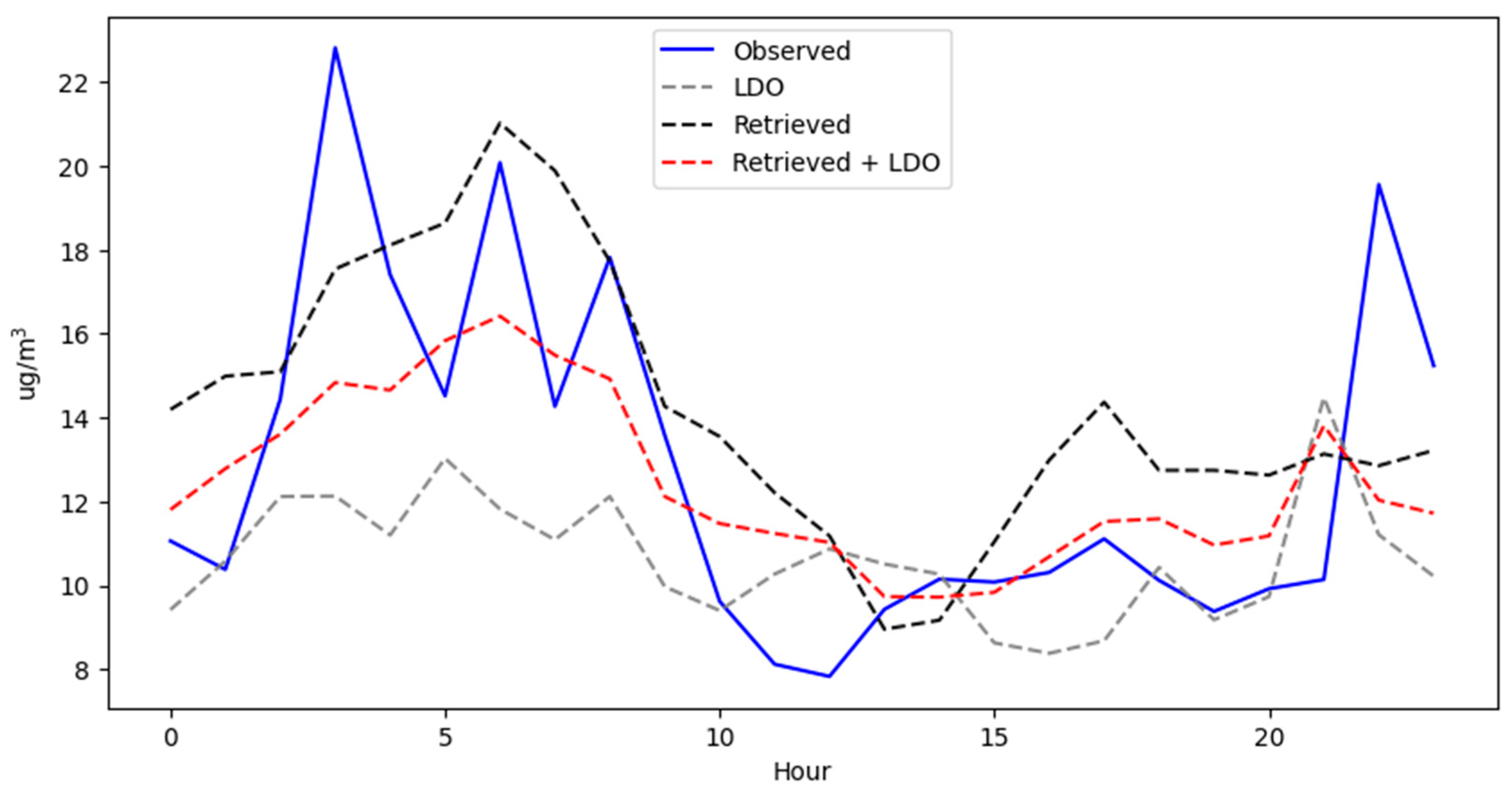
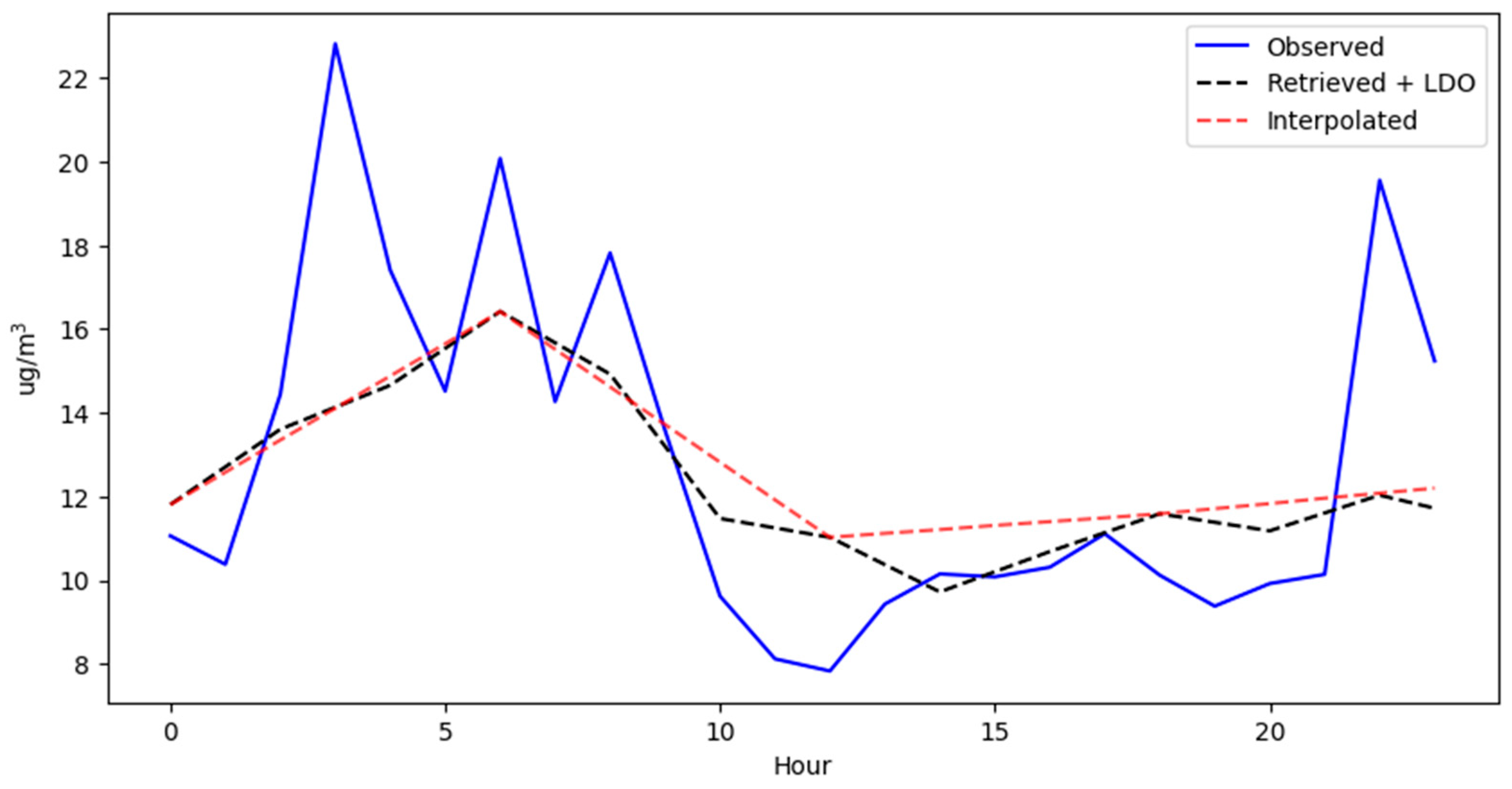
Bold represents the best result.

, it can be seen that in most monitoring stations, each element of the model contributes to improving the predictions, except for the case of the Espinar station, where the retrieved element, instead of reducing the RMSE, increases it. The optimal linear interpolation for each station was different: for Tala it was 6, for Uchumayo it was 5, and for Espinar it was 5.

According to

Table 6. Results in terms of MAPE.

Model	Station
	Tala	Uchumayo	Espinar
LDO	0.4597	0.7155	0.9415
Retrieved	1.0460	0.6734	0.8927
LDO + retrieved	0.6804	0.6535	0.7798
LDO + retrieved + linear interpolation	0.7101	0.6128	0.8922

Bold represents the best result.

, in terms of the MAPE, it can be seen that each element of the model does not contribute to the improvement in the model in the same way. For the Tala station, the elements that do not contribute to the improvement in the MAPE are retrieved to a greater extent and linear interpolation to a lesser extent. For the Uchumayo station, all elements contribute to the improvement. And, for the Espinar station, linear interpolation does not contribute to the improvement in the MAPE.

According to

Table 7. Results in terms of R presented by Formula (4).

Model	Station
	Tala	Uchumayo	Espinar
LDO	0.2926	0.2126	0.5602
Retrieved	0.0787	0.1912	0.1263
LDO + retrieved	0.3683	0.2624	0.5470
LDO + retrieved + linear interpolation	0.4282	0.2943	0.5332

Bold represents the best result.

, in terms of the R correlation, all the elements of the model contribute positively to improving the correlation level in the stations, except for linear interpolation at the Espinar station, which instead of increasing the correlation of LDO + retrieved (0.5470), decreases it to 0.5332.

4.2. Discussions

4.2.1. Comparison with Benchmark Models

The benchmark models implemented in this study include LSTM, BiLSTM, GRU, and BiGRU.

LSTM is a type of recurrent neural network that works with sequential or time series data, designed to solve the vanishing gradient problem through a memory cell that allows remembering or forgetting information, controlled by three main gates: the forget gate, input gate, and output gate.

BiLSTM is a variant of LSTM that processes information in two directions. One LSTM network reads the sequence forward, while another LSTM network reads it backward, and in the end, both representations are combined.

GRU is a recurrent neural network very similar to LSTM, but with a simpler and lighter structure. GRU has only two gates: a reset gate and an update gate.

BiGRU, similar to BiLSTM, is an extension of GRU that processes the sequence in two directions, forward and backward.

The hyperparameters used to implement the benchmark models are detailed in

Table 8. Hyperparameters of the benchmark models.

Model	Hyperparameters
LSTM	[50, 50, 50, 24], drop rate: 0.2, 0.2, 0.2, learning rate: 0.001
BiLSTM	[50, 50, 50, 24], drop rate: 0.2, 0.2, 0.2, learning rate: 0.001
GRU	[50, 50, 50, 24], drop rate: 0.2, 0.2, 0.2, learning rate: 0.001
BiGRU	[50, 50, 50, 24], drop rate: 0.2, 0.2, 0.2, learning rate: 0.001

.

All the implemented models use the same number of layers and neurons in each layer. They were implemented in the Jupyter IDE using the TensorFlow 2.18.0 library in Python language 3.11.7. The lookback for each model is 48 h. The models were compiled with ‘mse’ as the loss function and ‘adam’ as the optimizer, with a batch size of 50 and 50 training epochs. The results achieved are shown and described below.

According to

Table 9. Results in terms of RMSE. The benchmark models vs. the proposed model.

Model	Station
	Tala	Uchumayo	Espinar
LSTM	4.6232	4.9731	12.6984
BiLSTM	4.5846	4.6990	13.9089
GRU	4.4382	5.0418	14.3204
BiGRU	4.5198	4.3567	12.9484
Proposal	4.8469	4.5296	11.4006

Bold represents the best result.

, in terms of the RMSE, for the Tala station, GRU shows the lowest RMSE, equal to 4.4382 µg/m³, while the proposed model ranks last. For the Uchumayo station, BiGRU presents the lowest RMSE, equal to 4.3567 µg/m³, with the proposed model ranking second with an RMSE of 4.5296 µg/m³. Finally, for the Espinar station, the proposed model is the best, achieving the lowest RMSE, equal to 11.4006 µg/m³.

According to

Table 10. Results in terms of MAPE. The benchmark models vs. the proposed model.

Model	Station
	Tala	Uchumayo	Espinar
LSTM	0.4959	0.5545	0.7616
BiLSTM	0.4355	0.5163	0.7302
GRU	0.4499	0.5667	0.7771
BiGRU	0.4690	0.4725	0.7338
Proposal	0.7101	0.6128	0.8922

Bold represents the best result.

, in terms of the MAPE, for the Tala station, BiLSTM shows the lowest MAPE at 0.4355. For the Uchumayo station, BiGRU shows the lowest MAPE at 0.4725. And, for the Espinar station, BiLSTM shows the lowest MAPE at 0.7302. The proposed model shows the highest MAPE across all stations.

According to

Table 11. Results in terms of R presented by Formula (4). The benchmark models vs. the proposed model.

Model	Station
	Tala	Uchumayo	Espinar
LSTM	0.4823	0.2179	0.4740
BiLSTM	0.4981	0.2526	0.3373
GRU	0.5353	0.2527	0.2476
BiGRU	0.5182	0.3529	0.4347
Proposal	0.4282	0.2943	0.5332

Bold represents the best result.

, in terms of the R, for the Tala station, GRU shows the highest correlation at 0.5353, while the proposed model ranks last with 0.4282. For the Uchumayo station, BiGRU shows the highest correlation at 0.3529, while the proposal model ranks second with 0.2943. And, for the Espinar station, the proposed model shows the highest correlation at 0.5332.

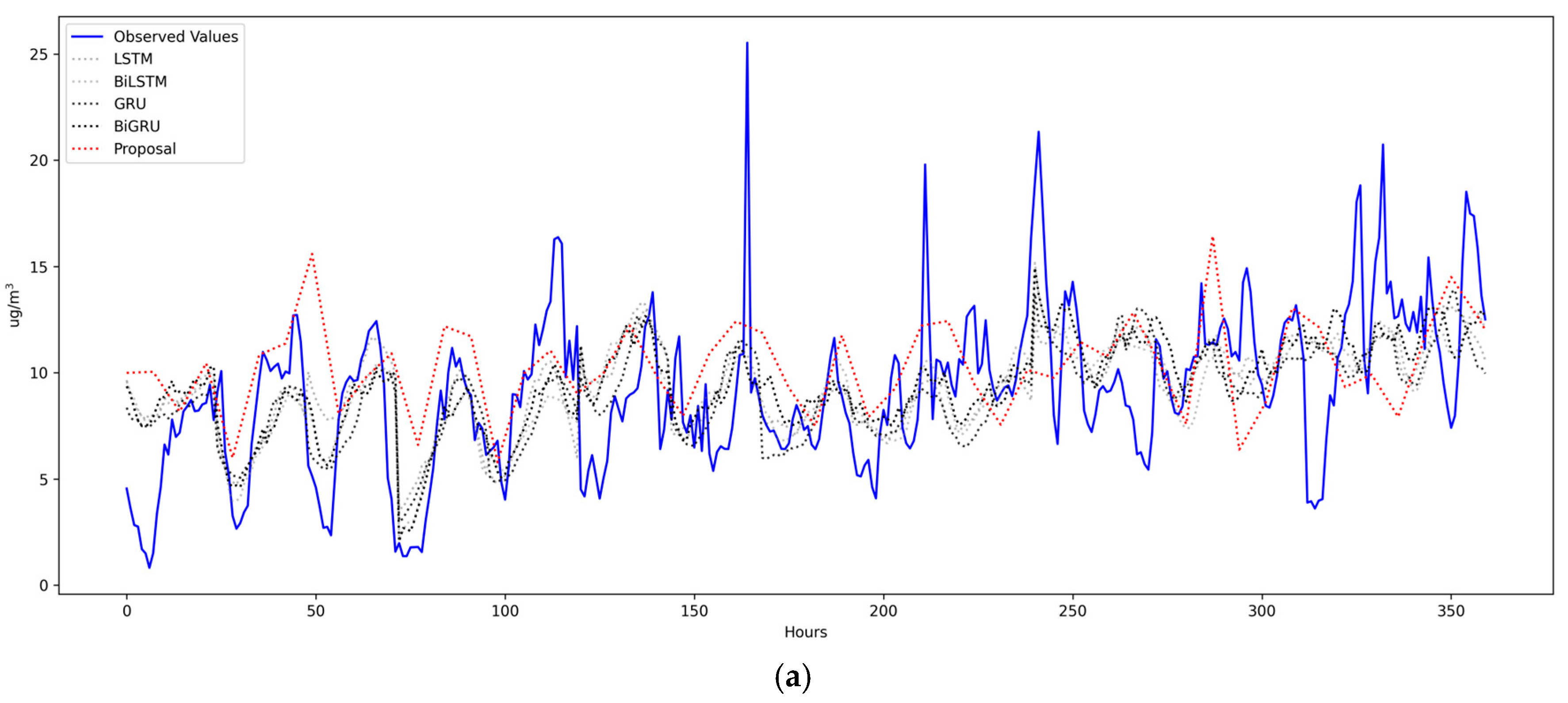
According to Figure 6, it can be observed that in the stations (Uchumayo and Espinar) where there is greater data variability, the proposed model shows a better performance than the benchmark models. However, in the Tala station, where data variability is lower, all the benchmark models outperform the proposed model.

In summary, each metric identifies different models as the best performers. This is due to the way each metric is calculated: the RMSE heavily penalizes large errors since it squares them, while the MAPE penalizes relative errors much more when the actual value is small.

4.2.2. Analysis of Prediction Errors

To analyze the errors in the predictions of the implemented models, the corresponding heatmaps were generated.

According to Figure 7a, for the Tala station, the absolute errors range between 0 and 80. All models show similar errors, concentrated around hour 2340 of the test data. However, the proposed model shows other clusters of high errors between hours 2700 and 2760, which definitely impacted the model’s performance for this station.

In contrast, for the Uchumayo station, according to Figure 7b, the absolute errors are smaller than those in the previous station, ranging between 0 and 25. Likewise, greater variability can be observed in the locations of the errors, but overall, all models show a similar number of errors, which is reflected in the RMSE, according to Table 6 shown earlier.

Finally, for the Espinar station, according to Figure 7c, the absolute errors are larger than those in the previous stations, ranging between 0 and 120. The distribution of the errors is similar for all models, with the highest concentrations between hours 2772 and 3234. However, it can be seen that the proposed model shows a lower concentration of errors compared to the benchmark models, which is reflected in the model’s performance.

At this point, it is important to highlight the difference between the predictions of the benchmark models, which are based on recurrent neural networks (RNNs), and the predictions of the proposed model. The benchmark models tend to produce higher errors at stations with greater variability, such as the Tala and Espinar stations, due to the nature of their architectures. During training, they minimize the average MSE, which leads the models to avoid predicting extreme values, peaks, or abrupt drops, resulting in smoother curves. In contrast, the proposed model applies smoothing based on linear interpolation; however, this is not necessarily applied to the extreme elements but rather to a set of predetermined values, allowing it to predict extreme values, as shown in Figure 6, thus producing better estimates for stations with greater variability.

4.2.3. Statistical Analysis

To determine whether one model is significantly better than another, in this section, the Kolmogorov–Smirnov (KS) test for two samples is applied. This test determines whether there is a significant difference between the proposed model and the benchmark models.

According to

Table 12. p-values for Kolmogorov–Smirnov (KS) test between proposed model and benchmark models.

Model	Station
	Tala	Uchumayo	Espinar
LSTM	8.56 × 10−33	1.75 × 10−104	9.94 × 10−86
BiLSTM	1.17 × 10−36	1.35 × 10−86	1.30 × 10−166
GRU	1.50 × 10−39	6.39 × 10−114	1.63 × 10−233
BiGRU	3.32 × 10−26	2.66 × 10−49	2.88 × 10−70

, it can be seen that all p-values are less than 0.05; therefore, the null hypothesis is rejected, and the alternative is accepted. This indicates that there is indeed a significant difference between the proposed model and the benchmark models across all monitoring stations.

As observed in Figure 5, the predictions of the recurrent neural network-based models are similar; however, they are not similar to those of the proposed model. This has been identified by the KS test, indicating a significant difference between the proposed model and the benchmark models, which does not imply that the proposed model is superior to the benchmark models, or vice versa.

4.2.4. Computational Cost

Table 13. Computational costs of implemented models in seconds.

Model	Station
	Tala	Uchumayo	Espinar	Avg
LSTM	310.32	215.37	377.20	300.96
BiLSTM	359.61	259.17	471.18	363.32
GRU	355.23	254.31	474.57	361.37
BiGRU	613.11	292.78	504.93	470.273
Proposal	0.4666	0.1831	0.5922	0.4140

Bold represents the best result.

shows the computational cost required to train each of the models implemented in this study, including the proposed model, on a computer with a Core i7-13700H processor at 2.40 GHz, 16 GB of RAM, running in a Windows 11 environment.

According to Table 13, it can be seen that the training costs in seconds of the benchmark models vary on average between 300.96 and 470.27 s, with LSTM being the least costly and BiGRU being the most costly. In contrast, the proposed model requires a much lower computational cost, averaging 0.4140 s, which represents 0.14% of the time required by LSTM and 0.09% of the time required by BiGRU.

Rapid and low-cost air quality forecasts, especially in mining areas, have direct and significant implications for public health and environmental management. First, having accessible predictive systems makes it possible to anticipate critical episodes of particulate matter pollution, facilitating the early issuance of health alerts to the exposed population. This can reduce the incidence of respiratory and cardiovascular diseases, particularly among vulnerable groups such as children, the elderly, and mining workers.

From an environmental perspective, these models contribute to the more efficient management of mining impacts, as they provide real-time information to adjust or temporarily halt operations during high-pollution events. Moreover, they promote transparency and citizen participation by allowing communities to access data and forecasts about their environment.

Likewise, it is important to highlight that the main weakness of complex deep learning models is the high computational cost required for their training. The proposed model greatly reduces this gap, making it a very good alternative for settings with limited computational resources.

4.2.5. Additional Tests

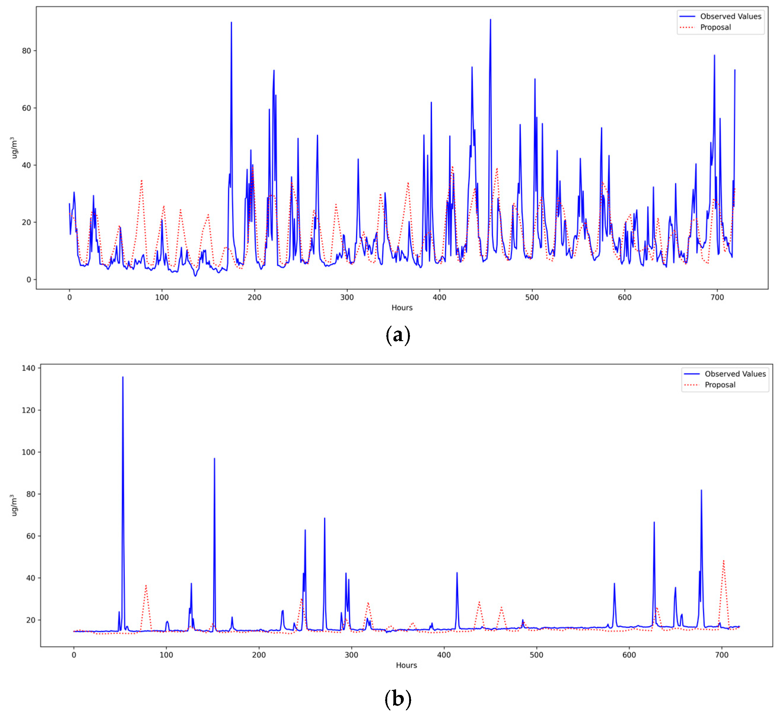
To improve the reliability of the results, additional tests were conducted using two new PM2.5 level datasets that do not correspond to mining areas but rather to urban areas, namely, the Pacocha and Pardo stations located in the city of Ilo, in southern Peru.

According to

Table 14. Results in terms of RMSE, MAPE, and R.

Station	RMSE	MAPE	R
Pacocha	11.3680	0.6323	0.3789
Pardo	10.2005	0.3152	0.2483

, it can be observed that the model’s performance is similar to that obtained for the three mining area datasets, with a noteworthy performance at the Pardo station, showing 10.2005 µg/m³ and a MAPE of 0.3152, which is higher than those obtained previously. This demonstrates that the model can be used not only for PM2.5 datasets in mining areas but also in other contexts. Figure 8 shows 720 predicted days for both datasets.

4.2.6. Limitations of the Study

This study has several limitations that could be addressed in future works to improve the results and be applied in other contexts. As can be seen from the results obtained, the prediction errors in all stations are still high, which indicates that there is still considerable room for improvement.

The first limitation lies in the number of datasets used, which is only three. For future works, datasets from other mines in Peru or other countries could be considered. Likewise, the monitoring stations are not located exactly at the mines but in the nearest cities.

Second, instead of using only two days for the retrieved data phase, a larger number of days could be considered. Similarly, instead of using an arithmetic mean, a weighted mean could be implemented according to the level of correlations. In this sense, instead of considering only 20 or 30 days of historical data for the search of similar series, this could be extended to a larger number of days.

Third, instead of linear interpolation, other types of interpolation could be considered, including Lagrange, Stineman, Spline, Kriging, Inverse Distance Weighting, or others.

Fourth, the proposed model is univariate, as it only considers PM2.5 levels; for future work, a multivariate model could be implemented by including other variables, such as wind speed, wind direction, humidity, precipitation, solar radiation, altitude, and vegetation cover. It is also important to highlight that a multivariate model will require a larger amount of data, as well as variables that are highly correlated with the PM2.5 levels to be predicted.

Fifth, the proposed model is implemented for the context of hourly data and predicts 24 h blocks. For daily, monthly data or frequencies lower than one hour, other adaptations would be needed, such as organizing the data by months, years, or similar.

5. Conclusions

In conclusion, it can be stated that the proposed model is a good alternative for predicting PM2.5 levels in mining areas in Peru. Out of the three datasets used, in two of them, Espinar and Uchumayo, the proposal produced the best estimates, ranking first and second, respectively, compared to the benchmark models. Another aspect that makes the proposal quite attractive compared to the other implemented models is the computational cost for its training, which represents less than 0.2% of that required to train models based on recurrent neural networks.