Application of Proximal Policy Optimization for Resource Orchestration in Serverless Edge Computing

Abstract

Serverless computing is a new cloud computing model suitable for providing services in both large cloud and edge clusters. In edge clusters, the autoscaling functions play a key role on serverless platforms as the dynamic scaling of function instances can lead to reduced latency and efficient resource usage, both typical requirements of edge-hosted services. However, a badly configured scaling function can introduce unexpected latency due to so-called “cold start” events or service request losses. In this work, we focus on the optimization of resource-based autoscaling on OpenFaaS, the most-adopted open-source Kubernetes-based serverless platform, leveraging real-world serverless traffic traces. We resort to the reinforcement learning algorithm named Proximal Policy Optimization to dynamically configure the value of the Kubernetes Horizontal Pod Autoscaler, trained on real traffic. This was accomplished via a state space model able to take into account resource consumption, performance values, and time of day. In addition, the reward function definition promotes Service-Level Agreement (SLA) compliance. We evaluate the proposed agent, comparing its performance in terms of average latency, CPU usage, memory usage, and loss percentage with respect to the baseline system. The experimental results show the benefits provided by the proposed agent, obtaining a service time within the SLA while limiting resource consumption and service loss.

1. Introduction

Edge computing has grown steadily in recent years. This technique consists of a computing paradigm based on the use of an infrastructure that is located at the edges of cloud systems and potentially close to users [1]. Devices in edge systems can be generic or specialized tools. For example, it is possible to find cameras or other Internet of Things (IoT) devices capable of collecting and processing data or computing and storage servers, as well as personal or mini computers. Edge computing is having considerable success, mainly due to the possibility of guaranteeing low latency in accessing virtualized computing resources, of processing data close to production nodes, and of securing sensitive data in specific portions of the network. For this reason, it is more and more present in the architecture of modern networks, such as 5G [2] and 6G [3] systems.

As always happens, the benefits come together with issues, which have stimulated research activities. The main cause of the problems faced is the limited availability of computing and storage resources [4]. Furthermore, the localized nature of the edge means that it can mainly be used by users present in the area close to the edge nodes.

Regarding the volume of available resources, its limitation has repercussions on the number of service instances that can be deployed at edge systems. Queuing theory results [5] demonstrate that the resource utilization coefficient determines the system service time, i.e., the latency necessary to receive a requested service. Therefore, if it is necessary to keep the service latency low, it is necessary to operate with a low service utilization coefficient. However, when a limited number of resources are available, this implies a low number of instantiable service instances.

The arrival process of service requests is determined by the users who are in the area of interest of the considered edge system. In specific scenarios, such as IoT or vehicular services, a high frequency of requests could cause service failures due to the unavailability of resources to instantiate new functions. Therefore, research in the edge computing field has been focused on ensuring sufficiently low values of the probability of failure to service. Furthermore, it is necessary to guarantee satisfactory latency values while maximizing the number of requests successfully served, i.e., define suitable service-level agreements (SLAs). Clearly, to guarantee a sufficiently low latency value, it is necessary to control the number of resources used by the service instances. This results in increasing the number of service instances activated in a time interval to serve those requests while maintaining the utilization coefficient at a predefined value.

A way to address this problem is to resort to a recent service implementation technique known as serverless computing [6,7]. It is event based and consists of instantiating minimal portions of code in stateless mode. These portions, called $functions$, are activated only for the time needed for their execution, thus resulting in significant savings in the use of infrastructure. In fact, when the execution of a function ends, it is removed and the associated resources are freed. If applications are organized into elementary functions that implement a single elementary part of the service, the savings are considerable. Typically, service providers make available an execution environment which allows running functions without the need for handling the underlying infrastructure. This way of accessing cloud services is known as serverless, and its implementation based on functions is referred to as Function as a Service (FaaS). Therefore, developers do not have to deal with any infrastructure management issues, including file system management, load balancing, and autoscaling.

To obtain good performance through the serverless technique, it is necessary to optimize the parameters that control its operation. In particular, the horizontal autoscaling of function instances typical of serverless technologies must be adapted to the characteristics of the edge system. In this paper, we will use the concept of state to comprehensively describe the system configuration and control it. The general research objective of this work is to use a reinforcement learning (RL) algorithm that has been shown to adapt to the state of edge systems and control operational parameters to drive the horizontal autoscaling events of functions. This algorithm is the Proximal Policy Optimization (PPO) algorithm. We show its ability to learn the system operation and to dynamically configure the optimal threshold value used to trigger horizontal autoscaling operations, typically set to the value of the percentage of CPU occupancy of instantiated functions. The purpose of the proposed control strategy is to minimize the number of functions to instantiate and, at the same time, to guarantee adequate latency values and successful access probability to services. In addition, we analyze the impact of system configurations on the achievable performance.

There are already some proposals that address similar problems, which will be surveyed in the Related Work section (Section 3). In our previous article [8], we showed the use of a reinforcement learning algorithm to minimize the average access latency in a serverless system. The algorithm used Q-learning. However, in order to allow the algorithm to converge, it was necessary to significantly simplify the state definition of the system. In this paper, we significantly improve the representation of the state, also including continuous variables, thus improving the generalization of the results and performance.

The analysis in this paper is experimental. It is based on the use of an edge computing cluster orchestrated through Kubernetes. In fact, Kubernetes is the most popular open-source container orchestrator. The serverless technology used is OpenFaaS [9], which is also one of the most popular serverless technologies. The resulting platform orchestrated by Kubernetes, in turn, configured at runtime by PPO, can be regarded as representative of artificial intelligence (AI)-controlled edge systems.

To sum up, the main contributions of this manuscript are the following:

• It highlights the typical problems to be addressed in edge systems when computing resources are managed through serverless technologies.
• It proposes a control system based on PPO to increase efficiency without penalizing latency.
• It compares the achievable performance of the proposal with a baseline system based on default Kubernetes parameters and comments critically on the results according to the dynamics of function invocations.

The paper’s organization is as follows: Section 2 introduces the serverless computing technique, the associated FaaS model, and the typical components of a serverless computing system. Section 3 presents research contributions about the usage of the serverless approach in edge computing systems managed by solutions based on AI. The proposed RL model, including a description of the used algorithm, the PPO algorithm, is presented in Section 4. Section 5 shows the experimental setup for performance evaluation and the results of lab experiments. Finally, Section 6 reports some concluding remarks.

2. Background on Serverless Computing

The cloud serverless deployment model shifts the burden of managing the infrastructure where services run to the provider. According to this model, resources are dynamically allocated to execute the customer software. This allows software developers to focus only on implementing and deploying the code to the production environment.

To exploit the potential of serverless computing, applications must be structured into elementary functions that are invoked in stateless mode. In this way, serverless services are often referred to as Function-as-a-Service (FaaS) services. In principle, a function should realize a simple task so that its execution is short-lived and its code easily recyclable. This method of accessing cloud resources tends to limit the number of resources used by customers and increases the number of applications instantiated by the provider. This mutual benefit has led to its current popularity.

Our research is based on the application of serverless technology to an edge computing system. With this system, we analyze the potential of a reinforcement learning algorithm, described in Section 4, to manage the horizontal scaling of the deployed functions. The architectural choices and the related achievable performance depend on the available features of both the technologies used and the environment where they are applied.

The system architectural model used in our experiments is shown in Figure 1. Before illustrating the individual components, we underline that the effect of the control consists of determining an optimal configuration for the number of running instances ($n_c$) of a given function. The value of $n_c$ is determined by a Kubernetes Horizontal Pod Autoscaler (HPA). The optimal value of $n_c$ allows the latency value specified in the Service-Level Agreement (SLA) to be obtained while the efficiency of usage of computing resources associated with the deployed functions is controlled.

The system includes the following functional elements, which are easy to to map into the components of some popular serverless platforms, such as OpenFaaS [9]:

• Computing cluster: This cluster is made of physical computing servers. In our experiments, we use just one server, which represents an IoT edge computing system. Clearly, it is necessary to deploy functions with an appropriate degree of isolation. In our system, they are deployed in containers implemented through the containerd runtime. Such containers are orchestrated through Kubernetes. For this reason, containers are included in Kubernetes $pods$. If there are $n_c$ function replicas running in the computing cluster, it is possible to assume that the service requests are equally distributed to these $n_c$ pods.
• Scheduler: This element is responsible for finding the most suitable node for a newly create pod to run on.
• Metrics Server: The role of this element is to collect resource metrics, such as memory and CPU load. These metrics are stored in a Log Repository made available to the HPA.
• Horizontal Pod Autoscaler (HPA): This element controls the number of active function replicas, and hence the number of running pods that implement the considered function. Therefore, the HPA allows the workload of each pod to be controlled in order to to match the desired load of computing cores. Thus, when the incoming load increases, the HPA instructs the controller to increase the number of running pods, and, when the load decreases, they are scaled back until the configured minimum number is reached. The HPA behavior can be influenced by some configuration parameters, in particular, the CPU threshold values for scaling the number of function instances up and down and their maximum and minimum values. To highlight their importance, we included a Configuration Parameters box in Figure 1.
• Controller Manager: This component manages the pod life cycle. It controls their status and enforces the instantiation of the number of running replicas received from the HPA.

To sum up, the HPA is a control loop implemented by the Controller Manager. At certain intervals, with a default value of 60 s but configurable down to a minimum of 15 s, the Metrics Server recovers raw metrics, exposing them as Resource Metrics, such as the CPU and memory usage of individual pods and nodes. Their values are averaged and sent to the HPA [10]. Considering CPU resource usage as the HPA autoscaling criteron, we carried out this work. Every 15 s, the HPA compares the collected CPU metric against the specified threshold and calculates the number of necessary function replicas at time interval $t+1$ by using the following formula [11]:

$$n_c(t+1)=⌈n_c\left(t\right){\displaystyle \frac{currentMetricValue}{Threshold}}⌉$$

(1)

In particular, the HPA calculates the currentMetricValue as a percentage of the used resources over those requested for the containers in each pod and compares this value with the desired percentage threshold ($Threshold$) to compute the desired number of replicas in (1), which ranges between a configurable minimum and a maximum number of replicas, configurable in the HPA definition (see the Configuration Parameter box in Figure 1).

The function startup latency is affected by a particular problem, commonly referred to as a cold start [12]. A cold start occurs when the system has to start a new function to fulfill a service request. In this case, it is necessary to configure the container runtime environment, download the function from a repository if it is not locally available, and deploy the function. The authors of [12] report some experimental values of cold start delays ranging from hundreds of ms to seconds. A possible approach for mitigating this problem consists of maintaining some instances running in the idle state and activating them when new requests arrive, thus creating a significantly lower service latency. This approach is known as a warm start. However, the cost of maintaining unused pods might not be affordable on edge systems, which are typically resource constrained. Some proposals make use of AI to predict service request arrivals, thus managing the instantiation of needed functions in advance [7,8]. However, the effectiveness of such an approach is highly dependent on the autocorrelation properties of the arrival process. Instead of making any assumption that could hinder the validity of our analysis, we use real traces, providing real temporal profiles of service requests to a serverless system [13].

3. Related Work

Papers [14,15] show some interesting experimental results regarding autoscaling in serverless systems. For evaluating the effects of autoscaling on performance, they consider success rate and response time. Paper [16] considers an edge computing system with serverless access. The analyzed system is implemented using Raspberry Pis devices. The paper illustrates a comparison of the performances obtainable using different platforms. In particular, AWS Greengrass, OpenFaaS, and Apache OpenWhisk were considered. The best results were obtained using OpenFaaS, although horizontal autoscaling was not used. Paper [17] shows a performance analysis of some open-source FaaS platforms. In particular, OpenFaaS, Fission, Kubeless, and Knative are used. Particular attention is paid to latency values. The functions used in the experiments are implemented using different programming languages such as Golang, Python, and NodeJS. The experimental analysis includes automatic scaling depending on the workload and available resources. A similar analysis regarding horizontal autoscaling is presented in [18]. FaaS access to a distributed edge system is analyzed in [19]. The analysis shown refers to centralized and distributed resource management algorithms. The experimental analysis includes an event simulator, and does not refer to any specific FaaS platform. The serverless approach is also considered in [20], applied to an edge system. In the proposal, the distribution of functions is controlled by analogy to a multi-armed bandit problem. Paper [21] shows a mathematical model of serverless processes. In particular, the authors use semi-Markov processes to represent serverless functionality. Validation is carried out by using measurements taken on an AWS Lambda-based system. In any case, these contributions do not concern the control of horizontal autoscaling functions using reinforcement learning algorithms.

The use of reinforcement learning in our proposal is motivated by its ability to manage distributed systems. This can also be deduced from other papers that analyze access to edge systems, even distributed ones, such as [19]. The analysis shown in the paper includes several resource management algorithms, both centralized and distributed. The experimentation uses an event simulator and does not refer to any particular FaaS technology. Serverless access is also analyzed in [20]. Again, it is applied to an edge system. In the considered system, the distribution of functions is modeled by referring to the multi-armed bandit problem. In our recent paper [22], we compared Deep Q-Network (DQN), PPO, and Advantage Actor–Critic (A2C). Despite the analysis being focused mainly on convergence time with a fixed arrival rate, PPO and A2C definitely outperformed DQN, and PPO exhibited a superior efficiency in resource utilization compared to A2C; thus, in this work, we focus on PPO.

A resource management proposal based on deep reinforcement learning for IoT systems is shown in [23]. The proposal in [24] combines Q-Learning and State–Action–Reward–State–Action (SARSA) to implement a control policy that makes use of fuzzy logic, with which computing resources are allocated to virtual machines. Reinforcement learning autoscaling is used in [25], making use of Docker Swarm-based orchestration. The use of Q-Learning to control the Kubernetes Horizontal Pod Autoscaler is shown in [26], although the autoscaler configuration is not detailed in the paper. A mathematical model of the Kubernetes Horizontal Pod Autoscaler is shown in [27]. The work includes a multi-prediction scaling engine used to control the probability of loss. Also, in this paper, no specific serverless platform is mentioned, nor are any real function invocation traces used. The authors of [28] present a reinforcement-learning-based model used to optimize the throughput in terms of request rate by tuning the serverless autoscaling. The research considers workload-based autoscaling for Knative, which is an open-source serverless platform based on Kubernetes. However, the work aims to minimize request losses only and does not consider a controlling service latency key performance indicator (KPI).

Resource-based autoscaling is adopted in [29], where Q-Learning, DynaQ, and Deep Q-Learning are considered to improve the performance of a CPU-intensive Kubeless application by adjusting the HPA CPU and memory usage thresholds. The research does not consider serverless traffic to train and evaluate the proposed solution. Moreover, no considerations of service losses are presented. Finally, Kubeless is an open-source serverless platform that is no longer maintained [30]. The approaches proposed in [29] suffer from convergence issues (see also [22]); thus, additional, synthetic traffic has to be used to train them. Paper [31] presents a multi-agent A3C (Asynchronous Advantage Actor–Critic) model aimed at minimizing a joint metric composed of the response time normalized to the SLA and lost requests. It compares the proposed model with the DQN, which exhibits known convergence problems, and some baseline methods, including the one based on a fixed threshold of CPU utilization equal to 50%, which is used in this paper as a baseline. However, apart from very low loads, where the baseline performance is even slightly better, the presented results clearly show that the proposed approach is not effective in enforcing the SLA. The authors of [32] present a very complex model based on joint usage of a long short-term memory model (LSTM) plus Proximal Policy Optimization (PPO). It is not oriented towards respecting the SLA on service time but towards minimizing losses. Furthermore, it aims to directly scale the number of instances, which is why it needs a predictive module such as the LSTM. Therefore, this model also appears to be unsuitable for creating a control system capable of guaranteeing the SLA in terms of service latency.

4. Reinforcement Learning Model

Reinforcement learning processes consists of algorithms executed by agents with the purpose of learning through continuous interaction with the environment [33]. Learning is based on subsequent decisions and related rewards. Reward values can be either positive or negative according to the outcomes determined by the selected actions. The general objective is, therefore, to learn the optimal strategy for selecting the actions that maximize the reward. Each learning iteration is implemented in consecutive steps. A step is an elementary interaction of the agent with the environment. Each interaction is associated with a state of the system. The latter is an exhaustive collection of parameter values that can be used to determine the dynamics of the system. An action could cause a state transition, which is associated with the related reward. In summary, during each iteration step, the agent selects an action, interacts with the environment and obtains a reward, associates the possible state transition with the reward, and adapts its behavior according to the collected results. Iterations are repeated over time to learn the system behaviour and thus improve the policy. Policies may be deterministic or statistic. In this paper, we consider statistic policies ${\pi }_{\theta }\left(a\right|s)$, associating a state $s\in \mathcal{S}$ with an action $a\in \mathcal{A}$, with $\mathcal{S}$ being the state space and $\mathcal{A}$ the action space. The policy parameters $\theta$ in the subscript are optimized during the training phase. In short, a stochastic policy is defined as a probability distribution over the possible actions that can be carried out when the system is in a specific state. The policy assigns a probability to each possible action, and, consequently, the agent selects an action as a function of these probabilities. This means that stochastic policies introduce a degree of randomness into the decision-making process. In fact, given a state, the agent may choose different actions with certain probabilities. This allows exploration of the state space to be implemented, thus helping the discovery of new and potentially better actions or strategies.

4.1. Basic Concepts of Bellman’s Equation

Research on reinforcement learning has been deeply influenced by the seminal work of Bellman on dynamic programming [34]. The core of Bellman’s work is the definition of the so-called Bellman equation, which is a recursive decomposition of a function named the “value function” ($v_{\pi }\left(s\right)$) in a state s (value of state s under policy $\pi$, i.e., the expected return) which has to be optimized, where the policy $\pi$ determines the transition from a state $s\in \mathcal{S}$ to the successor $s^{\prime }\in \mathcal{S}$. This equation defines the relationship between the value in a state (expected return) and that in the next states (successors) [33]:

$$\begin{array}{ccc}\hfill v_{\pi }\left(s\right)& =& {\mathbb{E}}_{\pi }\left[G_t|s_t=s\right]={\mathbb{E}}_{\pi }\left[r_{t+1}+\gamma v_{\pi }\left(s_{t+1}\right)\mid s_t=s\right]\hfill \\ \hfill & =& \sum _a\pi \left(a\right|s)\sum _{s^{\prime },r}p(s^{\prime },r|s,a)\left[r+\gamma v_{\pi }\left(s^{\prime }\right)\right],\hfill \end{array}$$

(2)

where ${\mathbb{E}}_{\pi }$ is expectation over policy, $G_t$ is the actual return following time t, $s_t$ is the system state at time t, $r\in \mathcal{R}$ is the immediate reward (whereas $r_t$ represents the reward received by the agent at time step t), and $\gamma$ is the so-called discount factor, which controls the importance of future rewards. The last term in the summation represents the contribution due to the immediate reward r plus the expected future returns from the next state $s^{\prime }$. This allows a recursive computation of the optimal policy to follow in a decision process aimed at optimizing that function. When applied to reinforcement learning, the function to optimize becomes the expected cumulative rewards accumulated over time for $t\in [0,T]$, i.e.,

$$G_t=\sum _{k=0}^{T-t-1}{\gamma }^k{r}_{t+k+1},$$

(3)

where the presence of a discount factor $\gamma \le 1$ forces the agent to focus more on immediate rewards than on future rewards. T is the episode length in time steps (horizon), and $T\to \infty$ for continuous tasks.

However, when applying dynamic programming methods to problems with large state space, as often happens in real case studies, the solution becomes unfeasible. Thus, it is necessary to resort to approximations of the value function and of the dynamic programming methods themselves. For instance, temporal difference (TD) learning [33] is a method able to directly approximate the value function of the Bellman equation without needing a model for the environment, combining both dynamic programming and Monte Carlo methods. In TD, inspiring to the Bellman equation (2), the current state value is approximated as follows:

$$V\left(s_t\right)\leftarrow V\left(s_t\right)+\alpha \left(r_{t+1}+\gamma V\left(s_{t+1}\right)-V\left(s_t\right)\right)$$

(4)

where $V\left(s_t\right)$ is the estimate of $v_{\pi }\left(s\right)$, and $\alpha$ is a parameter named the learning rate, which determines how much new information influences the old. In other words, since the environment model is not available, $v_{\pi }\left(s_{t+1}\right)$ is not known (see (2)), and it is approximated with $V\left(s_{t+1}\right)$, which can be estimated time step by time step. The quantity $r_{t+1}+\gamma V\left(s_{t+1}\right)$ is the TD target, whereas $\left(r_{t+1}+\gamma V\left(s_{t+1}\right)-V\left(s_t\right)\right)$ is the TD error, which is the difference between the target and the current estimate $V\left(s_t\right)$  [33]. The PPO algorithm inherits these concepts, making a further step forward, as described in the next section.

4.2. Proximal Policy Optimization

The Proximal Policy Optimization algorithm aims to optimize a policy trying to maintain a balance between the two general phases of exploration and exploitation. In its basic formulation, PPO works with the aim of maximizing an objective function and, at the same time, limiting the policy changes in order to avoid excessive changes.

The usefulness of PPO in configuring network intelligence mechanisms and for managing operational parameters in edge computing and wireless systems has already been demonstrated by recent research results [35,36].

PPO is performed by using the so-called surrogate objective function. It can be expressed as

$$L^{CLIP}\left(\theta \right)={\mathbb{E}}_t\left[min\left({\rho }_t\left(\theta \right){\widehat{A}}_t,\mathrm{clip}({\rho }_t\left(\theta \right),1-ϵ,1+ϵ){\widehat{A}}_t\right)\right]$$

(5)

where the parameter vector $\theta$ is updated in order to maximize the function. ${\mathbb{E}}_t$ indicates the expectation over time t. Clipping is used to avoid large updates. The formulation of this function includes the ratio ${\rho }_t\left(\theta \right)$ between the new policy ${\pi }_{\theta }$ and the old policy ${\pi }_{{\theta }_{\mathrm{old}}}$, used to update the current policy without making large changes as follows:

$${\rho }_t\left(\theta \right)={\displaystyle \frac{{\pi }_{\theta }\left(a_t\right|s_t)}{{\pi }_{{\theta }_{\mathrm{old}}}\left(a_t\right|s_t)}}$$

(6)

It represents a probability ratio, used to measure the difference between two policies (new and old) for a selected action $a_t$ in a state $s_t$. The practical average operation over time is performed by using the various time steps of the training process. ${\widehat{A}}_t$ is defined as the estimated advantage at time t. The advantage function represents the difference between the actual return and the estimated state value. It is used instead of the classic expected reward because it reduces the variance of the estimation. The clipping operation $\mathrm{clip}({\rho }_t\left(\theta \right),1-ϵ,1+ϵ)$ is used, as mentioned above, to limit drastic policy changes due to the effects of ${\rho }_t\left(\theta \right)$. In particular, the interval $[1-ϵ,1+ϵ]$ limits the possible policy deviations. The hyperparameter $ϵ$ determines the clipping width. Typical values are in the order of 0.1 or 0.2.

In more detail, the advantage function ${\widehat{A}}_t$ can be computed as follows (truncated version for $t\in [0,T])$:

$${\widehat{A}}_t={\delta }_t+\left(\gamma \lambda \right){\delta }_{t+1}+{\left(\gamma \lambda \right)}^2{\delta }_{t+2}+\dots +{\left(\gamma \lambda \right)}^{T-t-1}{\delta }_{T-1}$$

(7)

where ${\delta }_t=r_t+\gamma V\left(s_{t+1}\right)-V\left(s_t\right)$ is the temporal difference error (inspired by TD approximation in (4)), $\gamma$ is a discount factor, and $\lambda$ is a parameter that controls the bias–variance trade-off (typically set to $\lambda =1$). Thus, the estimated advantage function is the discounted sum of the temporal difference errors.

In order to define the final formulation of the loss function used during training, a specific loss for value functions is introduced:

$$L^{VF}\left(\theta \right)={\displaystyle \frac{1}{2}}{\mathbb{E}}_t\left[{\left(V_{\theta }\left(s_t\right)-V_t^{\mathrm{target}}\right)}^2\right]$$

(8)

This loss function value is a measure of the deviation between the model estimate $V_{\theta }\left(s_t\right)$ and the target value $V_t^{\mathrm{target}}$. Also, the value function is the result of a training process used to minimize the difference between the predicted value and the actual return. The value of the state estimates the expected return (i.e., cumulative future rewards) from a given state s. $V_t^{\mathrm{target}}$ estimates the value function in the state $s_t$, parameterized by $\theta$. The coefficient ${\displaystyle \frac{1}{2}}$ is just a scaling factor for the quadratic loss. The state value can be estimated using a parameterized algorithm, such as a neural network, producing $V_{{\theta }_v}\left(s\right)$, where ${\theta }_v$ represents the parameters of the estimator. Thus, the value function estimates the expected return from a given state s. This is performed by minimizing the value function loss $L^{\mathrm{VF}}\left({\theta }_v\right)$.

The total loss to minimize during training includes also an entropy term $S\left[{\pi }_{\theta }\right]\left(s_t\right)$, used to encourage additional exploration. This entropy “bonus” of the policy ${\pi }_{\theta }$ can be expressed following the usual form the the entropy definition:

$$S\left[{\pi }_{\theta }\right]\left(s\right)=-\sum _a{\pi }_{\theta }\left(a\right|s)log{\pi }_{\theta }\left(a\right|s)$$

(9)

Clearly, this term measures the uncertainty in the selection of actions. In synthesis, the complete loss function used in PPO is the following:

$$L\left(\theta \right)=L^{CLIP}\left(\theta \right)-c_1{L}^{VF}\left(\theta \right)+c_{2}S\left[{\pi }_{\theta }\right]\left(s_t\right)$$

(10)

where $c_1$ and $c_2$ are coefficients used to balance the three loss terms. It is worth noting that the entropy term is also useful for avoiding overfitting through the exploration of new strategies.

These parameters illustrated above are designed to gradually approach the optimal policy of the estimator, which is either a simple parameterized estimator or a more complex neural network, while preserving stability during training.

4.3. Proposed System Model

As with all systems using a reinforcement learning approach, it is necessary to define the state space $\mathcal{S}$, the action space $\mathcal{A}$, and the reward $r_t$. The state of the system is defined through the following quantities, which aim to provide a complete characterization of the execution environment:

1.

Mean response latency to a request issued to a running function during a time step ($l_m$);

2.

HPA CPU threshold value in percent (Threshold, as in (1));

3.

Number of function replicas within the cluster, evaluated as $n_c\left(t\right)$ in (1);

4.

Total usage of CPU by all active replicas in one minute, retrieved by the Metrics Server as $M_{CPU}\left(t\right)$;

5.

Total usage of RAM by all active replicas in one minute, retrieved by the Metrics Server as $M_{mem}\left(t\right)$;

6.

Average CPU usage in percent ($m_{CPU}\left(t\right)$) with respect to the guaranteed resources (requests), used as currentMetricValue for evaluating the number of replicas in (1);

7.

Average RAM usage ($m_{mem}\left(t\right)$) with respect to the guaranteed resources (requests) in percent;

8.

Number of requests received in a time step $N\left(t\right)$;

9.

Success rate of requests $S_R\left(t\right)$, that is, the fraction of $N\left(t\right)$ correctly served during the observed time step;

10.

Cosine of the angle computed using the current minute of the day;

11.

Sine of the angle computed using the current minute of the day.

The two final elements of the list are used to introduce time values with a period of one day. This is reasonable, as the arrival patterns of requests may exhibit a sort of periodicity, and this could be a simple-yet-effective way to capture it. In addition, two pairs of quantities are linearly dependent, that is, percentage usage of CPU and memory:

$$\begin{array}{cc}\hfill m_{res}\left(t\right)={\displaystyle \frac{M_{res}\left(t\right)}{po{d}_{res}\times n_c\left(t\right)}},& res=\{CPU,mem\}\end{array}$$

(11)

where $po{d}_{res}$ is the number of computing/memory resources guaranteed to each pod through the value of the requests parameter. Thus, the number of parameters composing the state of the system $s=\{s_1,...,s_k\}\in \mathcal{S}$ is $k=9$.

The agent action space $\mathcal{A}$ corresponds to the set of actions setting the HPA threshold value of the CPU load able to trigger autoscaling operations. We used a set composed of fixed, discrete values, $H_{th}$. We avoided selecting continuous values in the range of 0–100% to accelerate the learning process and avoid potential instabilities. All these actions (configuration of one of the $H_{th}$ values for the HPA threshold, i.e., $Threshold\leftarrow H_{th}\left(t\right)$ at step t, see also (1)) are compliant with any state s of the system.

For the training, we defined a maximum acceptable service latency equal to $\tau$ seconds as an SLA. If the observed service response time exceeds this value, the quality of service is assumed to be compromised. Therefore, the reward function $r_t$ takes into account the observed latency. In addition, it accounts also for service request losses. Since the traffic requests use the HTTP protocol, we assumed that a loss event occurs when the HTTP response code is different from 200 OK. Thus, we formalized the reward $r_t$ as a weighted sum of the latency contribution to the reward $r_t^{lat}$ and the loss contribution to the reward $r_t^{loss}$ as follows:

$$r_t^{lat}=\left\{\begin{array}{cc}{\displaystyle \frac{l_m}{\tau }},\hfill & l_m\le \tau \hfill \\ -{\displaystyle \frac{l_m-\tau }{\tau }},\hfill & l_m>\tau \hfill \end{array}\right.$$

(12)

$$r_t^{loss}=\left\{\begin{array}{cc}0,\hfill & S_R=1\hfill \\ -1,\hfill & S_R<1\hfill \end{array}\right.$$

(13)

$$r_t=w_1{r}_t^{lat}+w_2{r}_t^{loss}$$

(14)

where $l_m$ is the average service response time (over all requests received in one time step) as defined in the state space, $S_R$ is the fraction of correctly served requests (received in one time step) as defined in the state space, and $w_i$ is the weight of different contributions to the global reward $r_t$ to be used in (7).

The reward is expressed as a numerical value that is returned to the agent. It represents the quality of the outcomes due to the selected action. If the agent makes the best decisions that generate the optimal actions, it obtains the best reward that is obtainable in its state. Differently, if the actions are not optimal, the related reward values decrease, even reaching zero or negative values when the constraints on latency or loss are violated. Therefore, the reward is a measure of the achieved performance during the agent training phase.

The reward function used in this work was obtained by successive approximations in order to avoid stability problems. To obtain the final version, we conducted an in-depth analysis to identify the critical issues of each case. As is clear from the formulation $r_t^{lat}$, the objective was not to minimize the service latency, but to maintain the value within the SLA. We used an increasing reward function for latency values that approach the SLA without becoming lower than it (e.g., $l\le \tau$). From general queuing theory, when the utilization of a service node increases, this also generates an increase in service time. However, if the SLA is violated (i.e., $l_m>\tau$), a negative reward value must be set, decreasing with the service latency. This behavior is due the need to consider the further fundamental KPI in edge computing systems, which is the efficiency in the use of resources. In the system analyzed, the deployed function requires intensive use of the CPU. Therefore, it is necessary to keep processor usage high. This leads to the final version of the reward. Additionally, the total reward $r_t$ includes a penalty if a HTTP request is lost or not generating a proper response. The impact of these penalties depends on its weight, $w_2$, with respect to $w_1$.

5. Experimental Results

5.1. System Architecture and Testbed Technologies

This section presents our experimental setup with sufficient details to allow the interested reader to replicate the experiments shown. The edge computing testbed included two virtual machines (VMs), used to realize a mini Kubernetes (k8s) cluster composed of a master and a worker node. A detailed configuration of physical and virtual nodes is reported in

Table 1. Testbed specifications.

Device	CPU	RAM	Storage	OS	Software
Dell PowerEdge R630 1.3.6 (Tardis)	$2\times$ Intel(R) Xeon(R) CPU E5-2650 v3 @ 2.30 GHz: 40 threads	64 GB @2133 MT/s	279 GB (local) + 8 TB remote target iSCSI	Ubuntu 20.04 LTS	KVM + iSCSI client
Dell PowerEdge R630 2.4.3 (Saul)	$2\times$ Intel(R) Xeon(R) CPU E5-2640 v4 @ 2.40 GHz: 40 threads	128 GB @2133 MT/s	279 GB (local) + 8 TB remote target iSCSI	Ubuntu 20.04 LTS	KVM + iSCSI client
NAS QNAP TS-EC1280U (Hulk)	Intel(R) Xeon(R) CPU E3-1246 v3 @ 3.50 GHz: 8 threads	4 GB	72 TB (9 × 8 TB 3.5″ HDDs)	Firmware QTS 5.1.7.2770	SW for implementing iSCSI LUN (local unit number)
VM 1 (k8s Master)	4 vCPUs	12 GB	100 GB	Ubuntu 22.04.2 LTS	Kubernetes master SW, Docker, OpenFaaS, Python 3, StableBaseline3, Hey
VM 2 (k8s Worker)	24 vCPUs	32 GB	100 GB	Ubuntu 22.04.2 LTS	Kubernetes worker SW, Docker

. These VMs were executed through the KVM hypervisor on two Dell PowerEdge servers (Tardis and Saul, see Table 1). This way, we could parallelize the experimental campaign by doubling the number of experiments carried out simultaneously as both the VMs implementing a single cluster run on the same physical node. Although the two servers had different CPUs, their differences were very modest. We verified experimentally that differences in the obtained results were negligible. The VM storage was provided by an NAS, interconnected at the two servers through a 10 Gb/s switch. The decision to use a single worker node was made to emulate a single-node edge system, which is a quite common situation. However, since the cluster resources were abstracted from k8s and managed as a whole, this did not affect the generality of the results, which depended on the volume of resources available and not on the number of nodes.

We used OpenFaaS [9] as the serverless technology. It enables the creation and deployment of application functions. It has a container-based architecture based on the Docker runtime to run functions. Every function is packaged within a self-contained image. This structure can be easily customized by programmers, who can select any programming language. The integration of OpenFaaS with k8s is one of the key aspects of the technology as it allows the deployment of functions on any k8s cluster and allows it to benefit from its scalability properties. The interaction of these technologies is performed through an integrated API Gateway, which exposes the cluster functions to the outside. The API Gateway routes the received requests to the functions capable of serving them and manages the security policies. For the experimental testbed, we used the Community Edition of OpenFaaS, which is the only open-source version of the technology. This distribution offers a wide range of serverless features. However, it also has some important limitations compared to commercial distributions. In particular, the HPA present in the Community Edition allows each instantiated function to be replicated up to a maximum of five times. Therefore, our testbed made use of the HPA of k8s.

The PPO algorithm was implemented in the testbed using the Stable-Baselines3 [37] library. This is a library implemented in Python and provides the code of several RL algorithms. The library is compatible with Gymnasium [38] and PyTorch [39]. In particular, Gymnasium allows custom environments to be emulated through a rich set of open APIs. The environment implemented in the testbed included all the necessary components for the introduction of RL, such as the definitions of the state space, the possible actions, and the reward function, and those specific to the interaction with the RL agent.

To generate HTTP requests to the testbed at the desired frequency, we used the Hey [40] traffic generator. This tool facilitates the development and testing process by allowing clients to generate and send custom HTTP requests and replies to the requests with a set of output information with the request status code and other useful information, including response times. Hey also allows parallel request streams to be generated. In our experiments, we assumed that, on average, each Hey thread should send around $h_c=30$ HTTP requests during each minute (the time step); thus, we instantiated a number of parallel workers for Hey equal to ${\displaystyle \frac{N\left(t\right)}{h_c}}$.

For training and testing, we used data from the Azure Public Dataset, specifically, the Azure Functions Trace 2019 [13,41]. We selected the trace of one of the functions characterized by a challenging invocation profile. The traces of the dataset are organized in tables. Each row reports the function invocations during a day. The selected trace has an almost repetitive trend throughout the day, with some statistical fluctuations. Furthermore, during a day, there are rapid variations in the function invocation frequency, with peaks of about 1800 requests/minute, while there are also time intervals without any invocations, or very few. Thus, this trace is representative of many scenarios, and testing our model against it ensured quite general results. In our test, we used the traces related to the initial 5 days of the trace, in particular, the first 3 for training, and the last 2 for evaluation. In fact, we assessed that 3 days were enough for the convergence of the training phase, as already shown in our previous work [22]. In this way, we privileged the evaluation as much as possible so that the obtained results were evaluated on a significant volume of input data.

The experiments were carried out by using a compute-intensive function, which factors a number received in the HTTP request. For training and testing, we used a maximum latency threshold of $\tau =0.5$ seconds, which is the latency SLA. If the experimental latency exceeds this value, the service quality is considered unacceptable. Therefore, the reward function $r_t^{lat}$ takes negative values. The highest value is obtained for $l_m$ approaching $\tau$, as ${lim}_{l_m\to {\tau }^{-}}{r}_t^{lat}=1$, whereas ${lim}_{l_m\to 0}{r}_t^{lat}=0$. This means that the most favorable values for the service latency are those close to but still lower than $\tau$. As for the weights, we used $w_1=w2=1$. These values allow request losses to be avoided, which is the very primary KPI. In fact, whenever there is at least one HTTP request not served correctly, the loss component of the reward is set to $r_t^{loss}=-1$. This means that the only value of the service latency that can compensate this negative component of the reward is $l_m=\tau$, which would provide a global reward $r_t=0$, which is nearly impossible to obtain. In fact, a value of latency close but inferior to the SLA would give a slightly negative reward, whereas a value of latency slightly larger than $\tau$ would give a definitely negative global reward $r_t<-1.$ Instead, in the absence of losses, the latency value is the only quantity determining reward.

The set of percentage values used by the agent, configured in the HPA threshold of the CPU load, is equal to $H_{th}=\{10,30,50,70,90\}$. In spite of the limited number of selected values (there is a gap of multiples of 20% between each of them), they suitably cover the whole range and can provide satisfactory results, as shown in the next section. Increasing the number of values would require a significantly longer training time.

5.2. Numerical Results

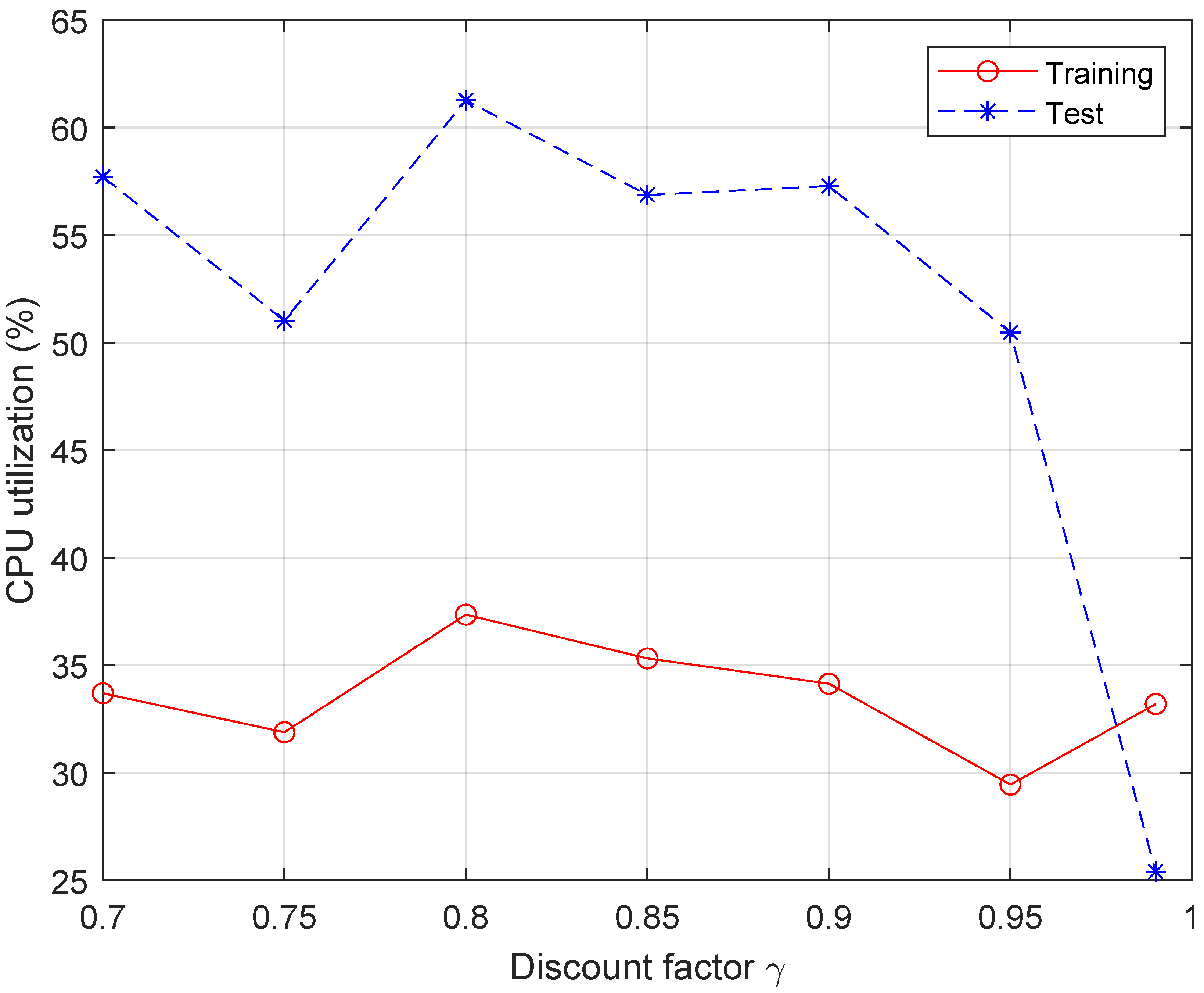
In this section, we illustrate the results of our experimental campaign, carried out on the testbed platform illustrated in the previous section. Results of our experiment are provided as Supplementary Materials, see the relevant section.

Table 2. Hyperparameters used for performance evaluation.

Hyperparameter	Value
Learning rate, $\alpha$	0.0003
Entropy coefficient, $c_2$	0.001
Discount factor, $\gamma$	0.7–0.99
Batch size for gradient update (mini-batch)	10
Number of steps per episode, T	10

lists the main common hyperparameters of the PPO algorithm. Most of values are the default ones for PPO in the used library. The only significant deviation is given by the discount factor $\gamma$. We present the results of our optimization, which identified $\gamma =0.8$ as the best value, which is significantly lower than the default value of 0.99.

As for system parameters, the k8s cluster was configured with a value of the downscale stabilization window ${\Delta }_S$, ranging in the interval between 30 and 300 s, kept fixed during each test. This way, the system results were more reactive in comparison to the default configuration, which is 5 min, which is used to avoid flapping of replicas when the metric values fluctuate. The Kubernetes manifest file, used to instantiate the deployment object managing the function pods, was configured by using the following values of the parameters requests and limits:

• requests: memory: “100 MB”, CPU: “100 m”;
• limits: values are reported in

  Table 3. Configurations of limits section in the Kubernetes deployment.

  Limits Configuration	HPA 120	HPA 250	HPA 500	HPA 750	HPA 1000
  CPU (millicores)	120	250	500	750	1000
  Memory (MB)	120	250	500	750	1000

  .

We verified that the value provided with the requests parameter was enough to run a single service request, and explored the impact on the PPO operation of the limits and downscale stabilization window.

Before presenting the results, we will explain why we do not present a configuration without specifying limits. Indeed, we carried out a number of experiments and verified that, in this case, some of the basic mechanism of Kubernetes are bypassed. In fact, when avoiding specifying the limits in the deployment manifest file, each pod can use, if needed, all the resources of the node in which it is running. OpenFaaS comes with a component for handling HTTP microservices named of-watchdog [42]. It implements a HTTP server listening on port 8080, and acts as a reverse proxy for running functions and microservices. It can be used independently or as the entry point for a container with OpenFaaS. In the streaming fork mode, which is the default one, it forks a process per request. Since all resources of the node can be used, these processes can be spread over all the available CPUs (24 in the case of the worker VM, see Table 1) even if a single function instance is deployed. Thus, they exhibit the best performance in terms of response latency and losses, which do not occur at all, as expected. We verified all this behavior experimentally. Therefore, although this configuration may seem optimal for a standalone testbed, it is not suitable for a service running on a cluster together with other tens or even hundreds of functions. In fact, although k8s is able to guarantee the number of resources specified in the requests section in the deployment manifest file of each function, the extra resources are managed without any control by the scheduler, possibly leading to undesired results. It is for this reason that all online tutorials recommend using limits (see, e.g., [43,44]). As a final comment, we note that, when tested with PPO, training does not converge in all the tested configurations since the system has all the resources needed to serve the requests and therefore cannot find preferential configurations in the different states.

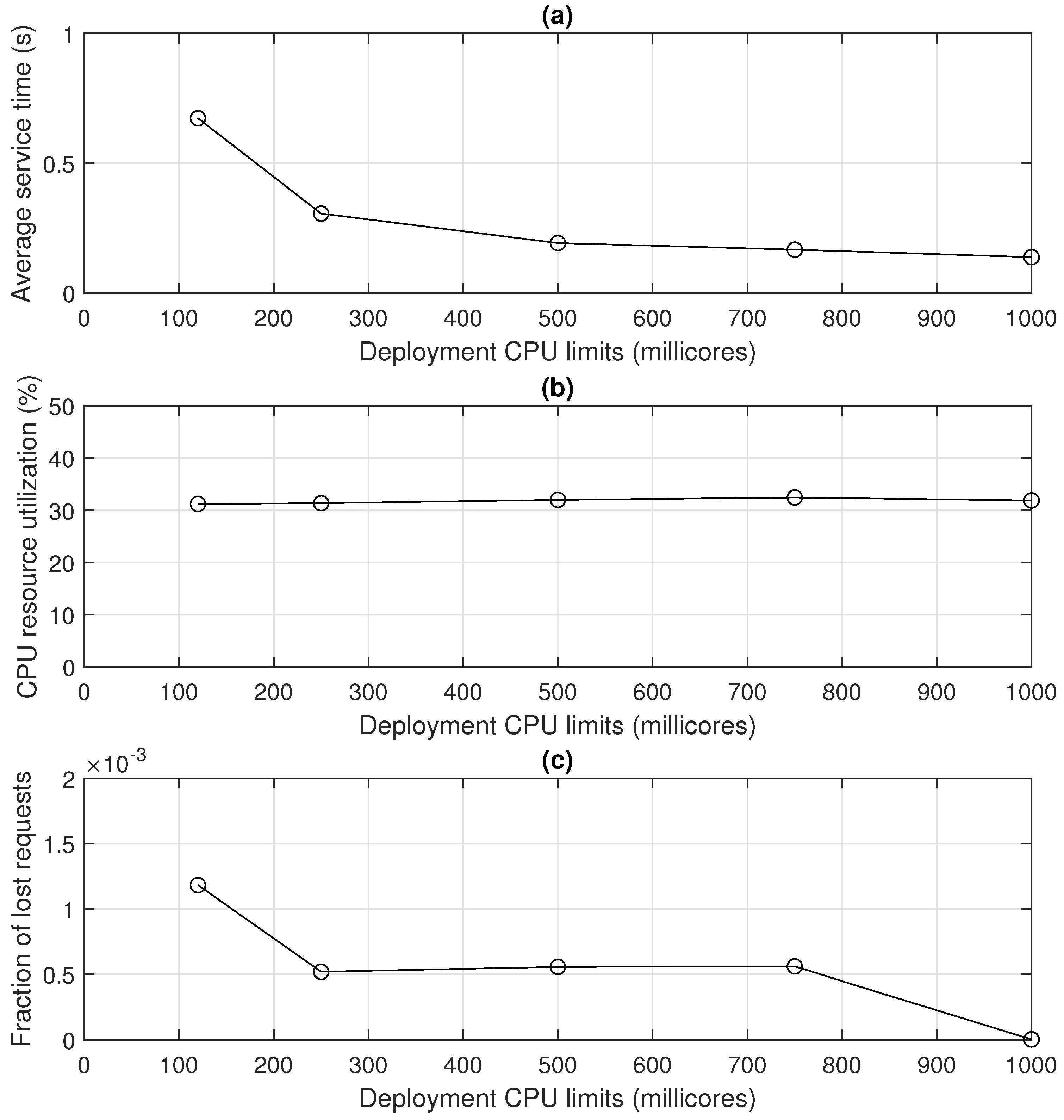
As for the baseline, it was configured with a HPA threshold of 50%, which is the typical value for k8s deployment, and default stabilization windows of 5 min. Also, in this case, we explored the impact of limits on the achievable performance. Before discussing the performance of the PPO, it is useful to discuss that of the baseline system, shown in Figure 2. The first comment is that, with a value of 120 m for the CPU limit, the baseline system cannot respect the SLA in terms of service latency. In fact, the resulting average value is in the order of 0.7 s, which is much higher than the SLA latency value, equal to 0.5 s. Also, request losses exhibit the highest value for this CPU limit. This is due to the behavior of the Linux scheduler, that is, the Completely Fair Scheduler (CFS) [45]. It operates with a default timeslice of 100 ms, during which it associates resources with all competing processes. With a very small peak value, it cannot provide enough resources during peak request times with the available resources. It has to wait for the k8s HPA scaling workflow to obtain more instances and then more resources. Instead, when more peak resources are available for the single pod, this phenomenon is highly mitigated. Thus, a good strategy is to assign requests as something more than the minimum to satisfy one request at time and rely on the peak limits to face extra, unexpected requests before the HPA enters into action. However, providing excessive peak resources could be not appropriate, as they are not guaranteed like those reserved with requests but can generate resource contentions with other applications. For peak resources larger than or equal to 250 m, we obtained acceptable service time and losses. However, the resource utilization was not satisfying at all, as it was practically fixed at 30%, regardless of the value of limits. Clearly, once a threshold of 50% has been set, average values larger than that are not expected, but they are close to it. However, the highly variable input process, combined with a high value of the stabilization window, set to 5 min, does not allow any acceptable values to be obtained. Since the utilization coefficient is evaluated with respect to the reserved resources, that is, those specified in the requests sections, and scaled by the number of replicas $n_c\left(t\right)$, they are valuable and should be used as much as possible. For this reason, we resorted to PPO.

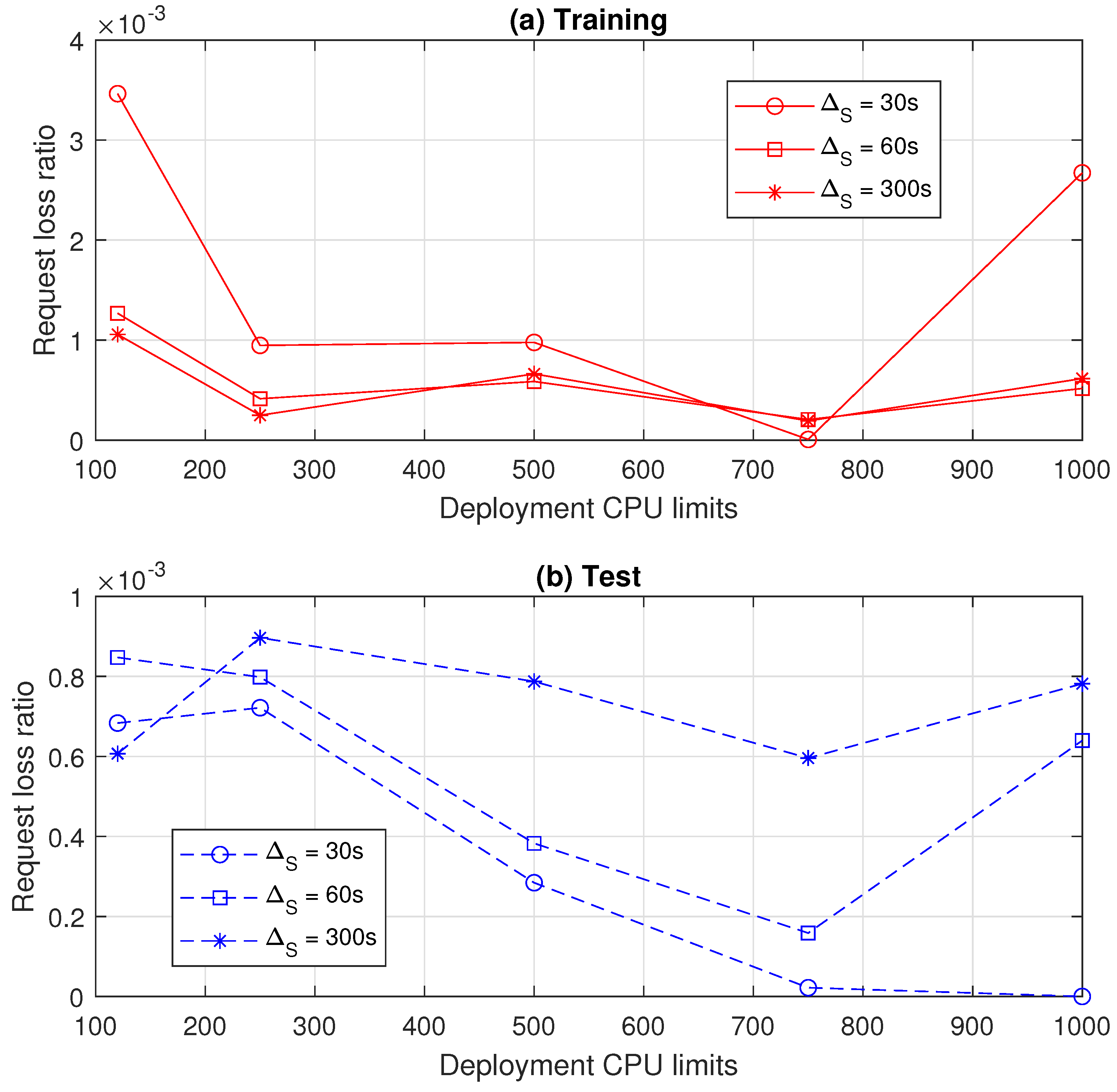
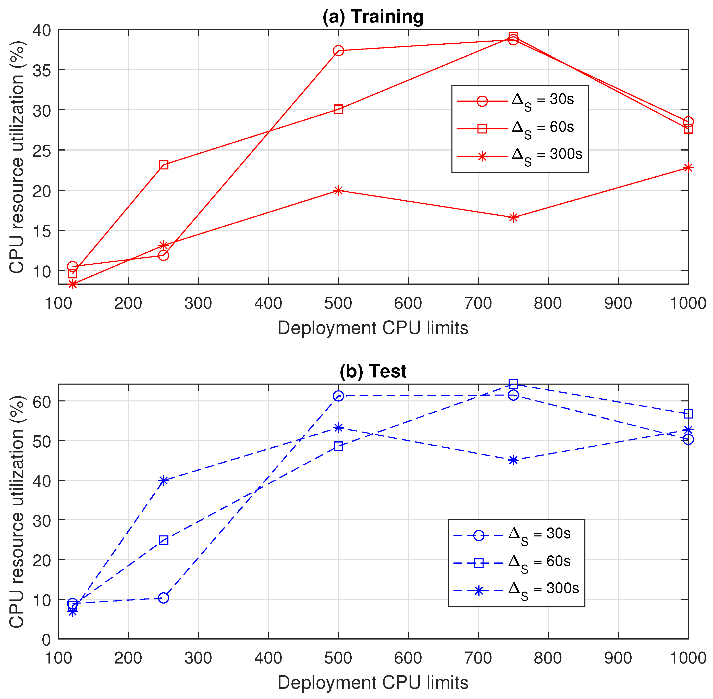
When PPO is used to set the HPA threshold of a serverless system running in a k8s cluster, we expect a number of improvements with respect to the usage of a fixed threshold on the percentage of CPU consumption. Figure 3, Figure 4, Figure 5 and Figure 6 show the performance of the system as a function of the values of the CPU limits reported in Table 3. All these figures are composed of two sub-figures. The top one (sub-figure (a)) is always relevant to the performance recorded during the training phase, whereas the bottom one (sub-figure (b)) is relevant to the test phase. Although the most important data are those obtained during the test phase, when the system is in operation, for the sake of completeness, we also report those collected during the training phase. In fact, even in operation, a possible deployment could include a separate small-scale testbed. It could be used to continue training as a digital twin of the operating cluster so as to periodically synchronize the platform in operation with the updated model obtained with the training platform.

Concerning the obtained results, we will start by discussing the service latency. It is evident from the analysis of Figure 3 that, in operation, all the considered configurations respect the SLA on the service time, equal to 0.5 s. This is a significant improvement over the baseline system, where, for a peak allocation of 120 m, the service latency is well beyond the SLA. In more detail, we can observe a decreasing trend in the value of CPU limits. On average, the lowest values are obtained with the largest value of ${\Delta }_S$. In fact, ${\Delta }_S$ acts as a hysteresis on the capability of the system to suddenly lower the number of allocated instances $n_c\left(T\right)$; the larger the stabilization window, the lower the reactivity in decreasing the number of allocated functions. Clearly, for smaller values of CPU limits, the Linux scheduler allocates fewer resources to serve incoming requests; thus, a longer service time is expected. In Figure 3b, it is possible to note some unexpected deviations with respect to the observed trend. This may be ascribed to the fact that our tests were carried out on a partially heterogeneous platform. Since the CPU of the Tardis server is older with slightly lower performance than the Saul one, some small deviations can happen. However, the obtained results do not alter the trend, which is clear. As for the training, with a peak value of 120 m, only the configuration with ${\Delta }_S=300$ s can respect the SLA on the service time due to its larger hysteresis effect. This is because, during training, not all the actions necessary to optimize the system performance are taken. Especially in the initial time steps, they are mainly taken to explore the system behavior through random sampling. Clearly, this may impact negatively on performance. As for the fraction of lost requests, all configurations in operations can keep this KPI below ${10}^{-3}$, which is definitely acceptable. During the training, the maximum values are obtained for ${\Delta }_S=30$ s, as expected, but, in any case, they are below $4\times {10}^{-4}$; thus, they are acceptable as well.

It is interesting to note that, in order to keep latency below the SLA, for small values of the CPU limits, the PPO forces the system to work with a very low threshold value. This average value is 10% for all values of ${\Delta }_S$ for CPU limits equal to 120 m and then gradually increases with the value of peak CPU. In fact, when the spare processing resources are enough to absorb peak requests, it is not necessary to suddenly scale the number of functions instances up. The value of the threshold regulates this mechanism, as shown in (1). In general, the largest values for the HPA threshold equal to 90% are reached for all values of ${\Delta }_S$. In particular, for 500 m, the peak rate ${\Delta }_S=30$ s and 60 s, and, for 750 m and 1000 m, the default value is 5 min. Consequently, with large values of the threshold, we expect large values of CPU utilization. Figure 6 shows that the best values are obtained when ${\Delta }_S$ is small (30 s and 60 s) as it makes the system more reactive in de-allocating unnecessary resources, thus increasing their utilization efficiency. In more detail, the highest values are reached for CPU peaks of 500 m (${\Delta }_S=30$ s) and 750 m (${\Delta }_S=30$ s and 60 s). Although for CPU limits equal to 750 m and ${\Delta }_S=60$, it is possible to reach a utilization of CPU resources equal to about 64%, we think that the configuration with CPU limits equal to 500 m and ${\Delta }_S=30$ is a more interesting working point. In fact, the achieved utilization is beyond 61%, but the system manages resources in a more conserving way, using a lower peak value, which is always preferable. We stress that the utilization in the baseline system is only 30%. Thus, by using PPO, it is possible not only to keep the service latency always under control, but also to reach a 100% improvement in terms of resource utilization, which is definitely a great result.

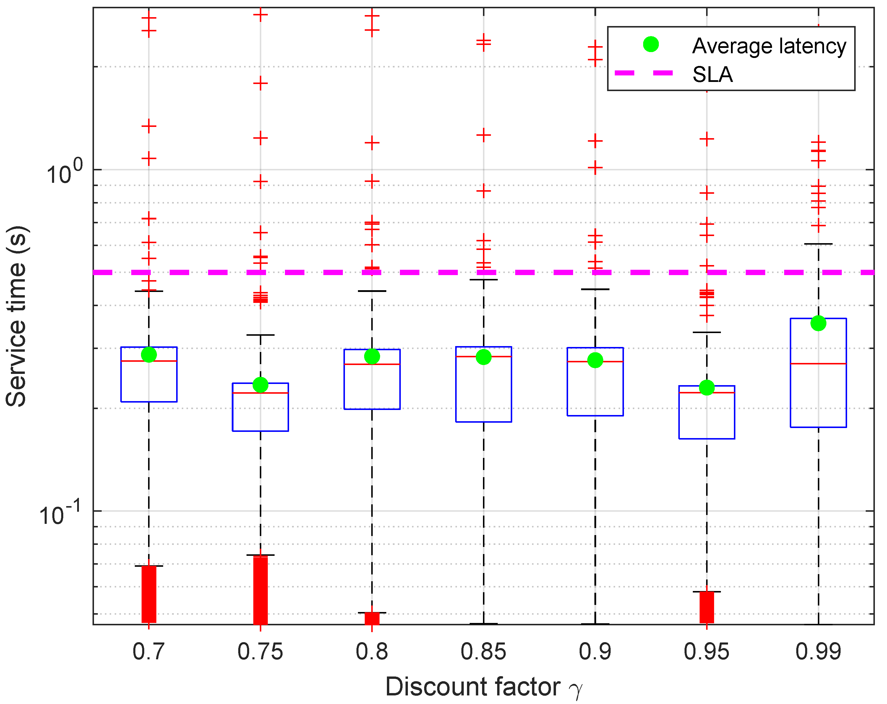
Finally, having identified the most suitable working configuration, we will analyze how PPO hyperparameters affect it. We verified that the parameter with the largest impact on performance is the discount factor $\gamma$. Thus, we present the performance study of the configuration with CPU limits equal to 500 m and ${\Delta }_S=30$ s by varying $\gamma$ from 0.7 to 0.99, which is the default value. Figure 7 presents the boxplot of service latency (test phase) as a function of $\gamma$. It is evident that the average value is compliant with the SLA for all configurations. Thus, let us consider the CPU utilization, shown in Figure 8. In this case, it is evident that the best value is obtained with $\gamma =0.8$, reaching the value of 61% identified in Figure 6, whereas the default one is the most problematic. In more detail, it is interesting to note that, for the selected configuration, most of the dynamics of the service latency are within the SLA, not just the average values, with only a few outliers going beyond it. Instead, for the default configuration, the maximum value is also beyond the SLA, in addition to the presence of outliers.

6. Conclusions

This paper explores the applicability of the PPO reinforcement learning strategy to managing edge computing systems. In order to maximize the efficiency of resource usage, a serverless deployment methodology was applied on an edge computing node orchestrated by Kubernetes. In this scenario, PPO is used to control the horizontal autoscaling procedures of computationally intensive functions. It turns out that PPO can operate the system respecting the SLA constraint in terms of service latency. It happens in all configurations of CPU peak configuration at the expense of potentially low utilization efficiency. However, in some configurations, not only are SLA values respected in terms of service latency and request losses, but a significant improvement in terms of resource utilization is obtained. In particular, the utilization value reaches 60%, which is double the value achievable with the baseline system.

Finally, we showed through an analysis relevant to sensitivity to hyperparameters, that default values in the available libraries are not always suitable for achieving the best performance.

Future works will focus on the extension of this research to deployment of multiple functions with the aim of identifying the most suitable deployment strategy to guarantee SLA and, at the same time, optimize global resource utilization. This will involve the characterization of possible resource contentions between functions of the same or different applications.

References

1. ETSI. Multi-Access Edge Computing (MEC); Framework and Reference Architecture. In ETSI ISG MEC, ETSI GS MEC 003 V2.1.1; ETSI: Valbonne, France, 2023. [Google Scholar]
2. Hassan, N.; Yau, K.L.A.; Wu, C. Edge Computing in 5G: A Review. IEEE Access 2019, 7, 127276–127289. [Google Scholar] [CrossRef]
3. Li, Q.; Ding, Z.; Tong, X.; Wu, G.; Stojanovski, S.; Luetzenkirchen, T.; Kolekar, A.; Bangolae, S.; Palat, S. 6G Cloud-Native System: Vision, Challenges, Architecture Framework and Enabling Technologies. IEEE Access 2022, 10, 96602–96625. [Google Scholar] [CrossRef]
4. Hong, C.H.; Varghese, B. Resource Management in Fog/Edge Computing: A Survey on Architectures, Infrastructure, and Algorithms. ACM Comput. Surv. 2019, 52, 1–37. [Google Scholar] [CrossRef]
5. Kleinrock, L. Theory, Volume 1, Queueing Systems; Wiley-Interscience: Hoboken, NJ, USA, 1975. [Google Scholar]
6. Aslanpour, M.S.; Toosi, A.N.; Cicconetti, C.; Javadi, B.; Sbarski, P.; Taibi, D.; Assuncao, M.; Gill, S.S.; Gaire, R.; Dustdar, S. Serverless Edge Computing: Vision and Challenges. In Proceedings of the 2021 Australasian Computer Science Week Multiconference, Dunedin, New Zealand, 1–5 February 2021. ACSW’21. [Google Scholar] [CrossRef]
7. Raith, P.; Nastic, S.; Dustdar, S. Serverless Edge Computing—Where We Are and What Lies Ahead. IEEE Internet Comput. 2023, 27, 50–64. [Google Scholar] [CrossRef]
8. Benedetti, P.; Femminella, M.; Reali, G.; Steenhaut, K. Reinforcement Learning Applicability for Resource-Based Auto-scaling in Serverless Edge Applications. In Proceedings of the 2022 IEEE International Conference on Pervasive Computing and Communications Workshops and other Affiliated Events (PerCom Workshops), Pisa, Italy, 21–25 March 2022; pp. 674–679. [Google Scholar] [CrossRef]
9. OpenFaaS: Open Function as a Service. Available online: https://www.openfaas.com/ (accessed on 22 July 2024).
10. Nguyen, T.T.; Yeom, Y.J.; Kim, T.; Park, D.H.; Kim, S. Horizontal Pod Autoscaling in Kubernetes for Elastic Container Orchestration. Sensors 2020, 20, 4621. [Google Scholar] [CrossRef] [PubMed]
11. Kubernetes Horizontal Pod Autoscaler. Available online: https://kubernetes.io/docs/tasks/run-application/horizontal-pod-autoscale/ (accessed on 22 July 2024).
12. Wang, L.; Li, M.; Zhang, Y.; Ristenpart, T.; Swift, M. Peeking Behind the Curtains of Serverless Platforms. In Proceedings of the 2018 USENIX Annual Technical Conference (USENIX ATC 18), Boston, MA, USA, 11–13 July 2018; pp. 133–146. [Google Scholar]
13. Shahrad, M.; Fonseca, R.; Goiri, I.; Chaudhry, G.; Batum, P.; Cooke, J.; Laureano, E.; Tresness, C.; Russinovich, M.; Bianchini, R. Serverless in the Wild: Characterizing and Optimizing the Serverless Workload at a Large Cloud Provider. In Proceedings of the 2020 USENIX Annual Technical Conference (USENIX ATC 20), USENIX Association, Online, 15–17 July 2020; pp. 205–218. [Google Scholar]
14. Mohanty, S.K.; Premsankar, G.; di Francesco, M. An Evaluation of Open Source Serverless Computing Frameworks. In Proceedings of the 2018 IEEE International Conference on Cloud Computing Technology and Science (CloudCom), Nicosia, Cyprus, 10–13 December 2018; pp. 115–120. [Google Scholar] [CrossRef]
15. Palade, A.; Kazmi, A.; Clarke, S. An Evaluation of Open Source Serverless Computing Frameworks Support at the Edge. In Proceedings of the 2019 IEEE World Congress on Services (SERVICES), Milan, Italy, 8–13 July 2019; Volume 2642-939X, pp. 206–211. [Google Scholar] [CrossRef]
16. Javed, H.; Toosi, A.; Aslanpour, M.S. Serverless Platforms on the Edge: A Performance Analysis. In New Frontiers in Cloud Computing and Internet of Things; Springer: Cham, Swizerland, 2022; pp. 165–184. [Google Scholar] [CrossRef]
17. Balla, D.; Maliosz, M.; Simon, C. Open Source FaaS Performance Aspects. In Proceedings of the 2020 43rd International Conference on Telecommunications and Signal Processing (TSP), Milan, Italy, 7–9 July 2020; pp. 358–364. [Google Scholar] [CrossRef]
18. Li, J.; Kulkarni, S.G.; Ramakrishnan, K.K.; Li, D. Understanding Open Source Serverless Platforms: Design Considerations and Performance. In Proceedings of the 5th International Workshop on Serverless Computing, Davis, CA, USA, 9–13 December 2019; WOSC’19; pp. 37–42. [Google Scholar] [CrossRef]
19. Ascigil, O.; Tasiopoulos, A.; Phan, T.; Sourlas, V.; Psaras, I.; Pavlou, G. Resource Provisioning and Allocation in Function-as-a-Service Edge-Clouds. IEEE Trans. Serv. Comput. 2021, 15, 2410–2424. [Google Scholar] [CrossRef]
20. Pinto, D.; Dias, J.P.; Sereno Ferreira, H. Dynamic Allocation of Serverless Functions in IoT Environments. In Proceedings of the 2018 IEEE 16th International Conference on Embedded and Ubiquitous Computing (EUC), Bucharest, Romania, 29–31 October 2018; pp. 1–8. [Google Scholar] [CrossRef]
21. Mahmoudi, N.; Khazaei, H. Performance Modeling of Serverless Computing Platforms. IEEE Trans. Cloud Comput. 2022, 10, 2834–2847. [Google Scholar] [CrossRef]
22. Femminella, M.; Reali, G. Comparison of Reinforcement Learning Algorithms for Edge Computing Applications Deployed by Serverless Technologies. Algorithms 2024, 17, 320. [Google Scholar] [CrossRef]
23. Sheng, S.; Chen, P.; Chen, Z.; Wu, L.; Yao, Y. Deep Reinforcement Learning-Based Task Scheduling in IoT Edge Computing. Sensors 2021, 21, 1666. [Google Scholar] [CrossRef] [PubMed]
24. Arabnejad, H.; Pahl, C.; Jamshidi, P.; Estrada, G. A Comparison of Reinforcement Learning Techniques for Fuzzy Cloud Auto-Scaling. In Proceedings of the 2017 17th IEEE/ACM International Symposium on Cluster, Cloud and Grid Computing (CCGRID), Madrid, Spain, 14–17 May 2017. [Google Scholar] [CrossRef]
25. Rossi, F.; Nardelli, M.; Cardellini, V. Horizontal and Vertical Scaling of Container-Based Applications Using Reinforcement Learning. In Proceedings of the 2019 IEEE 12th International Conference on Cloud Computing (CLOUD), Milan, Italy, 8–13 July 2019; pp. 329–338. [Google Scholar]
26. Horovitz, S.; Arian, Y. Efficient Cloud Auto-Scaling with SLA Objective Using Q-Learning. In Proceedings of the 2018 IEEE 6th International Conference on Future Internet of Things and Cloud (FiCloud), Barcelona, Spain, 6–8 August 2018; pp. 85–92. [Google Scholar] [CrossRef]
27. Toka, L.; Dobreff, G.; Fodor, B.; Sonkoly, B. Machine Learning-Based Scaling Management for Kubernetes Edge Clusters. IEEE Trans. Netw. Serv. Manag. 2021, 18, 958–972. [Google Scholar] [CrossRef]
28. Schuler, L.; Jamil, S.; Kuhl, N. AI-based Resource Allocation: Reinforcement Learning for Adaptive Auto-scaling in Serverless Environments. In Proceedings of the 2021 IEEE/ACM 21st International Symposium on Cluster, Cloud and Internet Computing (CCGrid), Los Alamitos, CA, USA, 10–13 May 2021; pp. 804–811. [Google Scholar] [CrossRef]
29. Zafeiropoulos, A.; Fotopoulou, E.; Filinis, N.; Papavassiliou, S. Reinforcement learning-assisted autoscaling mechanisms for serverless computing platforms. Simul. Model. Pract. Theory 2022, 116, 102461. [Google Scholar] [CrossRef]
30. Kubeless. Available online: https://github.com/vmware-archive/kubeless (accessed on 22 July 2024).
31. Mampage, A.; Karunasekera, S.; Buyya, R. A Deep Reinforcement Learning based Algorithm for Time and Cost Optimized Scaling of Serverless Applications. arXiv 2023. [Google Scholar] [CrossRef]
32. Agarwal, S.; Rodriguez, M.A.; Buyya, R. A Deep Recurrent-Reinforcement Learning Method for Intelligent AutoScaling of Serverless Functions. IEEE Trans. Serv. Comput. 2024, 1–12. [Google Scholar] [CrossRef]
33. Sutton, R.S.; Barto, A.G. Reinforcement Learning: An Introduction; A Bradford Book: Cambridge, MA, USA, 2018. [Google Scholar]
34. Bellman, R.E. Dynamic Programming; Princeton University Press: Princeton, NJ, USA, 1957. [Google Scholar]
35. Lee, G.H.; Park, H.; Jang, J.W.; Han, J.; Choi, J.K. PPO-Based Autonomous Transmission Period Control System in IoT Edge Computing. IEEE Internet Things J. 2023, 10, 21705–21720. [Google Scholar] [CrossRef]
36. Zhang, R.; Xiong, K.; Lu, Y.; Fan, P.; Ng, D.W.K.; Letaief, K.B. Energy Efficiency Maximization in RIS-Assisted SWIPT Networks With RSMA: A PPO-Based Approach. IEEE J. Sel. Areas Commun. 2023, 41, 1413–1430. [Google Scholar] [CrossRef]
37. Stable-Baselines3 Library. Available online: https://stable-baselines3.readthedocs.io/en/master/ (accessed on 22 July 2024).
38. Gymnasium Library. Available online: https://gymnasium.farama.org/index.html (accessed on 22 July 2024).
39. PyTorch Library. Available online: https://pytorch.org/ (accessed on 22 July 2024).
40. Hey traffic Generator. Available online: https://github.com/rakyll/hey (accessed on 22 July 2024).
41. Azure Functions Trace. Available online: https://github.com/Azure/AzurePublicDataset (accessed on 22 July 2024).
42. OpenFaaS of-Watchdog. Available online: https://github.com/openfaas/of-watchdog (accessed on 22 July 2024).
43. HPA Should Use the Limits Instead of Requests. Available online: https://github.com/kubernetes/kubernetes/issues/108026 (accessed on 22 July 2024).
44. Horizontal Pod Autoscaler Should Use Resource Limit as Its Base for Calculation. Available online: https://github.com/kubernetes/kubernetes/issues/72811 (accessed on 22 July 2024).
45. Completely Fair Scheduler. Available online: https://docs.kernel.org/scheduler/sched-design-CFS.html (accessed on 22 July 2024).
Figure 1. General model of a controlled serverless computing cluster.
Computers 13 00224 g001
Figure 2. Performance of the baseline system without the reinforcement learning in terms of (a) service latency, (b) resource utilization (CPU), and (c) fraction of lost requests.
Computers 13 00224 g002
Figure 3. Performance of PPO-driven serverless edge system in terms of service latency as a function of the value of CPU limits for both (a) training and (b) test.
Computers 13 00224 g003
Figure 4. Performance of PPO-driven serverless edge system in terms of fraction of lost service requests as a function of the value of CPU limits for both (a) training and (b) test.
Computers 13 00224 g004
Figure 5. Average value of the HPA threshold in the PPO-driven serverless edge system as a function of the value of CPU limits for both (a) training and (b) test.
Computers 13 00224 g005
Figure 6. Performance of PPO-driven serverless edge system in terms of CPU utilization efficiency as a function of the value of CPU limits for both (a) training and (b) test.
Computers 13 00224 g006
Figure 7. Boxplot of service latency for PPO-driven serverless edge system (CPU limits set to 500 m, Δ S = 30  s) as a function of the discount factor γ in the test phase.
Computers 13 00224 g007
Figure 8. CPU utilization efficiency for PPO-driven serverless edge system (CPU limits set to 500 m, Δ S = 30  s) as a function of the discount factor γ for both training and test phases.
Computers 13 00224 g008