Abstract
Monitoring bus driver behavior and posture in urban public transport’s dynamic and unpredictable environment requires robust real-time analytics systems. Traditional camera-based systems that use computer vision techniques for facial recognition are foundational. However, they often struggle with real-world challenges such as sudden driver movements, active driver–passenger interactions, variations in lighting, and physical obstructions. Our investigation covers four different neural network architectures, including two variations of convolutional neural networks (CNNs) that form the comparative baseline. The capsule network (CapsNet) developed by our team has been shown to be superior in terms of efficiency and speed in facial recognition tasks compared to traditional models. It offers a new approach for rapidly and accurately detecting a driver’s head position within the wide-angled view of the bus driver’s cabin. This research demonstrates the potential of CapsNets in driver head and face detection and lays the foundation for integrating CapsNet-based solutions into real-time monitoring systems to enhance public transportation safety protocols.
1. Introduction
Increasing traffic density necessitates safer public transport, where the role of drivers remains pivotal despite advancements in advanced driver-assistance systems (ADASs) like emergency braking [1]. Focusing on driver attention and cognitive load is vital for optimizing working conditions and enhancing accident prevention. In this context, CapsNets have been integrated into professional camera-based driver monitoring systems (DMSs) for public transport in order to improve safety. Despite a decrease in overall usage, buses still represent a significant part of European public road transport, with over 108 thousand million passengers and 97 thousand million passenger-kilometers in 2022, according to relevant data from selected countries—Bulgaria, the Czech Republic, Germany, Estonia, Croatia, Lithuania, Hungary, Poland, Portugal, and Romania (Table 1) [2].

Table 1.
Data concerning motor coaches, buses, and trolley buses in selected EU countries (Bulgaria, the Czech Republic, Germany, Estonia, Croatia, Lithuania, Hungary, Poland, Portugal, and Romania) [2].
Research has highlighted several key factors contributing to bus accidents, including the negligence of bus operators, driver errors, and external elements like weather and road conditions. It has been noted that monitoring driver behavior through passive or active interventions can significantly enhance the safety of bus transportation [3]. Various factors can contribute to inattention, including distractions (visual, auditory, physical, or cognitive) and drowsiness. Drowsiness may be caused by various factors, such as insufficient sleep, poor health, or prolonged driving in dull environments, and can result in physiological inattention [4]. Factors like boredom, fatigue, monotony, and sleep deprivation are known to amplify accident risks. This is because they tend to reduce the driver’s attention, thereby hindering information processing and decision-making capabilities, which are crucial for reacting effectively in emergencies [5]. Studies on accidents and simulated driving have indicated that alertness can diminish during daytime as well, particularly on lengthy, unvarying routes [6]. Errors are more prevalent during monotonous driving, where low task demands and stimulus levels lead to reduced attention. Various systems incorporating psychological tests and different physiological sensors have been developed to monitor and detect driver behaviors. These systems employ methods such as vehicle-based measures, behavioral measures, and physiological measures [7].
Vehicle sensors have been increasingly used to detect driving patterns and behaviors. For example, driving patterns can be discerned from vehicle sensor data during a single turn [8]. Deep learning framework that analyze CAN-BUS data have been successful in identifying different driving behaviors [9]. Monitoring systems in vehicles that utilize principal component analysis can track fuel consumption, emissions, driving style, and driver health in real-time effectively [10]. Additionally, energy efficiency in rail vehicles is being optimized by detecting energy losses [11]. Behavioral studies, such as those utilizing the Driver Behavior Questionnaire, suggest that professional drivers typically engage in safer driving practices, yet face a higher risk of accidents due to longer driving times [12]. Driver characteristics, like comfort levels, can influence driving performance [13]. Large-scale studies on bus drivers using psychometric evaluations like the Multidimensional Driving Style Inventory and Driver Anger Scale have underscored the importance of identifying safe versus unsafe drivers [14]. A strong correlation has been found between vehicle data and physiological driver signals, suggesting that vehicle data can be highly indicative of driver behavior [15]. With high-quality cameras, eye-tracking systems can measure cognitive load by observing fixation frequency, pupil diameter, and blink rates [16]. Experienced drivers show distinct fixation patterns in driving scenarios compared to novices [17]. Pupil size is also an indicator of attention levels and can vary with the difficulty of tasks or the type of interface used, such as touchscreens [18].
Driver fatigue and distraction can be assessed through biometric signals, steering patterns, or monitoring the driver’s face [19]. It has been found that an elevated heart rate may indicate that a driver is engaged in more complex or additional tasks [20]. Heart rate variability, corroborated by electroencephalography, has also been utilized to gauge driver drowsiness [21]. Additionally, wearable devices that measure galvanic skin responses have been successfully used to detect driver distraction accurately in real-world driving conditions [22]. Recent developments include single-channel EEG systems that analyze data using small time windows and single-feature calculations, making them more suitable for integration into embedded systems due to reduced processing and storage needs [23]. Muscle fatigue, measured using electromyograms (EMGs), has also been used to monitor driver alertness, with appropriate methodologies outlined [24].
The most common type of DMS is camera-based, utilizing computer vision to recognize facial features. This approach is less intrusive for drivers and fits seamlessly into mass production processes for vehicles. According to EU Regulation 2019/2144, starting in 2024, all new vehicles in Europe must include a system that warns against driver drowsiness or distraction [25]. Visual sensors, including RGB and IR cameras, collect naturalistic driving data, encompassing driver interactions, behaviors, and the vehicle’s interior environment. These data can be used to monitor hand movements, body posture, facial expressions, and signs of distraction or drowsiness [26]. Face detection technologies are broadly categorized into feature-based and learning-based methods, with the latter typically being more robust, albeit more resource-intensive. These technologies can achieve detection rates of over 80% in controlled environments [27]. The current challenge is to prove these algorithms’ effectiveness and demonstrate their practical benefits. In the future, improved facial recognition technology could significantly enhance road safety. However, the accuracy of these technologies depends on various factors, such as the camera’s angle, vibrations, lens cleanliness, obstructions, lighting, and overall optical performance. It is vital to consider and address these factors during data collection and processing to ensure reliable results.
The critical role of computer vision and machine learning was mentioned by the creators of a DMS that enhances road safety [28]. Others took this a step further by detecting driver distraction using a CapsNet, an AI-based method that has outperformed traditional machine learning models. This research categorized various distractions and tested the model under different conditions, offering substantial improvements in autonomous vehicle safety [29]. Building on previous models, some have explored the utilization of modified CapsNets for identifying distracted driver behavior [30]. While CNNs have been commonly used, CapsNets are advantageous as they maintain the spatial relationships between features. By adding an extra convolutional layer to the CapsNet structure, the authors achieved a high accuracy of 97.83% with hold-out validation. However, the model’s performance decreased to 53.11% with leave-one-subject-out validation, suggesting the need for further research to improve the model’s generalization capabilities.
Automatic face localization, a key challenge in computer vision, often employs object detection algorithms like Faster-RCNN [31], SSD [32], and various versions of YOLO [33] for effective face detection. However, recognizing the unique characteristics of human faces, specific deep architectures have been designed for higher accuracy in diverse conditions. MTCNN is a notable scientific method utilizing a cascaded structure with deep convolutional networks for precise face and landmark detection [34]. Faceness-Net improves detection when occlusions are present by using facial attributes in its network, highlighting the continuous evolution and specialization in face detection technologies [35]. The integration of feature pyramid networks (FPNs) in face detection, particularly for small faces, has been a notable advancement. The selective refinement network (SRN) utilizes FPNs for feature extraction, introducing a two-step approach in classification and regression to enhance accuracy and reduce false positives [36]. SRNs include selective two-step classification (STC) and selective two-step regression (STR) modules for efficient anchor filtering and adjustment. Another approach, RetinaFace, employs FPNs in a single-stage, multi-task face detector, handling aspects like face scores, bounding boxes, facial landmarks, and 3D face vertices [37]. Additionally, CRFace and HLA-Face address specific challenges in high-resolution images and low-light conditions, respectively, reflecting the significant progress that has been achieved in face detection technology [38].
Deep face recognition (FR) architectures have evolved rapidly, following trends in object classification. Starting with AlexNet [39], which revolutionized the ImageNet competition with its deep structure and innovative techniques like ReLU and dropout, the field progressed to VGGNet [40], which introduced a standard architecture with small convolutional filters and deeper layers. GoogleNet then brought in the inception module, merging multi-resolution information [41]. ResNet further simplified the training of deep networks by introducing residual mapping [42]. Finally, SENet [43] improved representational power with the squeeze-and-excitation block, enhancing channel-wise feature responses.
Advancements in FR architectures have paralleled those in object classification, leading to more profound, controllable networks. DeepFace pioneered this with a nine-layer CNN, achieving 97.35% accuracy on labeled faces in the wild (LFW) using 3D alignment [44]. FaceNet implemented GoogleNet and a novel triplet loss function, reaching 99.63% accuracy [45]. VGGface further refined this approach with a large-scale dataset and VGGNet, attaining 98.95% accuracy [46]. SphereFace introduced a 64-layer ResNet and angular softmax loss, boosting performance to 99.42% on LFW [47]. The end of 2017 saw the introduction of VGGface2, a diverse dataset enhancing the robustness of FR models [48]. MobiFace, an optimized deep-learning model for mobile face recognition, was also introduced [49]. It achieves high accuracy (99.73% on LFW, 91.3% on Megaface) with reduced computational demands, addressing the limitations of mobile device resources. This development marked a significant step in mobile-based face recognition technology.
In this article, we will conduct a comparative study between the conventional dynamic routing algorithm and our proposed routing method within two different network architectures. Our ultimate research aim is for our CapsNet model to demonstrate robust performance in professional settings, such as DMS for public transportation. This paper presents the initial phase of our research, which enhances the robustness of the head location detection algorithm and paves the way for further assessments of the model’s speed and computational efficiency in practical applications. This approach not only addresses the detection of head position with precision but also accounts for the various challenges associated with monitoring bus drivers during the performance of their duties.
This paper is structured as follows: Section 2 clarifies the mathematical background necessary to understand the theory of capsule networks and briefly describes the introduced routing algorithm. Following this, we describe the dataset we created, designed specifically for our long-term goals. Finally, we present and detail the generated neural network models. Section 3 clarifies the context in which the networks are trained, highlighting the most critical parameters, and presents and visualizes the results in detail. Section 4 discusses the achieved results. Finally, Section 5 presents the conclusion.
2. Materials and Methods
This study focuses on identifying the bus drivers’ faces under various conditions, including sudden movements, active interactions between drivers and passengers, and environmental challenges such as changing light conditions and physical obstructions. The core objective is to explore the feasibility of applying this monitoring approach in practical scenarios. Furthermore, we aim to examine the effectiveness and resilience of capsule networks enhanced by a tailored routing process.
Verma et al. introduced a pioneering system for the real-time monitoring of driver emotions, employing face detection and facial expression analysis [50]. This system utilizes two VGG-16 neural networks; the first extracts appearance features from the face images while the second network extracts geometrical features from facial landmarks. On another front, Jain et al. presented a method based on capsule networks for identifying distracted drivers, and this demonstrated superior performance in real-world environments when compared to traditional CNN approaches [29]. Ali et al. contributed to the field by creating a dataset for use in various experiments concerning driver distraction. They proposed an innovative method that leverages facial points-based features, particularly those derived from motion vectors and interpolation, to identify specific types of driver distractions [51]. Lastly, Liu et al. offered an extensive review of face recognition technologies, discussing the challenges associated with face recognition tasks. They outlined the principal frameworks for face recognition, including geometric feature-based, template-based, and model-based methods, comparing various solutions while underscoring the significance of and prevailing challenges in the domain of face recognition [52].
Our previous work focused on accurately identifying 15 facial keypoints, laying the groundwork for advanced facial recognition techniques [53]. Building upon this foundation, the present study leverages CapsNets to precisely detect the head’s orientation. Our approach is designed to deliver dependable results amidst the challenging and variable conditions encountered in bus driving scenarios. We highlight the implementation of CapsNets in real-world DMSs for public transportation, thereby advancing the field of research in this domain.
2.1. Capsule Network Theory
CapsNets represent an evolution of traditional neural networks, addressing several of their well-documented challenges [54,55]. The fundamental distinction between CapsNets and conventional neural networks lies in their primary structural unit. Unlike neural networks, which are constructed from neurons, CapsNets are built using entities known as capsules. Table 2 outlines the principal differences between these capsules and the classical artificial neurons.
Table 2.
Differences between a capsule and a neuron.
A capsule within a network can be conceptualized as a collection of intricately linked neurons that engage in substantial internal computation and encapsulate the outcomes of these computations within an n-dimensional vector, which serves as the capsule’s output. Notably, the capsule’s output diverges from the output of a conventional neuron as it does not represent a probability value. Instead, the magnitude of the output vector conveys the probability value associated with the capsule’s output, while the vector’s orientation encodes various attributes pertinent to a specific task. For instance, in the context of detecting a human face, lower-level capsules might be tasked with identifying facial components—such as eyes, nose, or mouth—whereas a higher-level capsule would be dedicated to the holistic task of face recognition. The neurons within these lower-level capsules capture and encode certain intrinsic properties of the object, including its position, orientation, color, texture, and shape.
A distinctive feature of capsule networks is that they eschew the employment of pooling layers or analogous mechanisms for reducing dimensionality between layers. Instead, these networks adopt a ‘routing-by-agreement’ mechanism, whereby the output vectors from lower-level capsules are directed towards all subsequent higher-level capsules. This process involves a comparative analysis between the output vectors of the lower-level capsules and the actual outputs from the higher-level capsules. The routing mechanism’s primary objective is to modulate the intensity of information flow between capsules, facilitating enhanced connectivity among features that are closely related.
Consider a lower-level capsule, denoted by , and a higher-level capsule, denoted by . The input tensor of capsule is determined as follows:
where represents a weighting matrix that is initially populated with random values, and signifies the pose vector of the -th capsule. The coupling coefficients are derived using a straightforward softmax function, expressed as follows:
where symbolizes the logarithmic probability that capsule will couple with capsule , and with being set to zero at the start [54,55].
The aggregate input for capsule is the cumulative weighted sum of the prediction vectors, as is shown below [54,55]:
In the architecture of the capsule network, each layer outputs vectors, with the length of these vectors determining the probability. It is imperative to apply a non-linear squashing function to these vectors before the probability can be assessed, where the squashing function is defined as follows:
The routing mechanism is essential for elucidating the interactions between the layers of the capsule network [54,55]. The dynamic routing algorithm, referred to as Algorithm 1, is essential for the updating values and for the determination of the output capsule vector.
| Algorithm 1. Routing algorithm [54] | |
| 1: | procedure ROUTING (, , ) |
| 2: | for all capsule in layer and capsule in layer : |
| 3: | for iterations do |
| 4: | for all capsule in layer : |
| 5: | for all capsule in layer : |
| 6: | for all capsule in layer : |
| 7: | for all capsule in layer and capsule in layer : |
| 8: | return |
2.2. Proposed Capsule Routing Mechanism
In our previous work [56], we introduced a simplified routing algorithm for capsule networks and demonstrated its performance in a variety of classification tasks. In this paper, we use the same optimization solution. However, we use it for detection rather than classification. Within the domain of capsule network research, our investigations reveal that the input tensor plays a pivotal role in the efficacy of the dynamic routing optimization procedure, significantly influencing the resultant tensor. The computation of the output vector incorporates the input tensor on two occasions as follows:
where is the squashing function, and signifies the softmax function [56]. To improve the routing mechanism between lower-level and upper-level capsules, we suggest the modifications to the routing algorithm outlined below [56]:
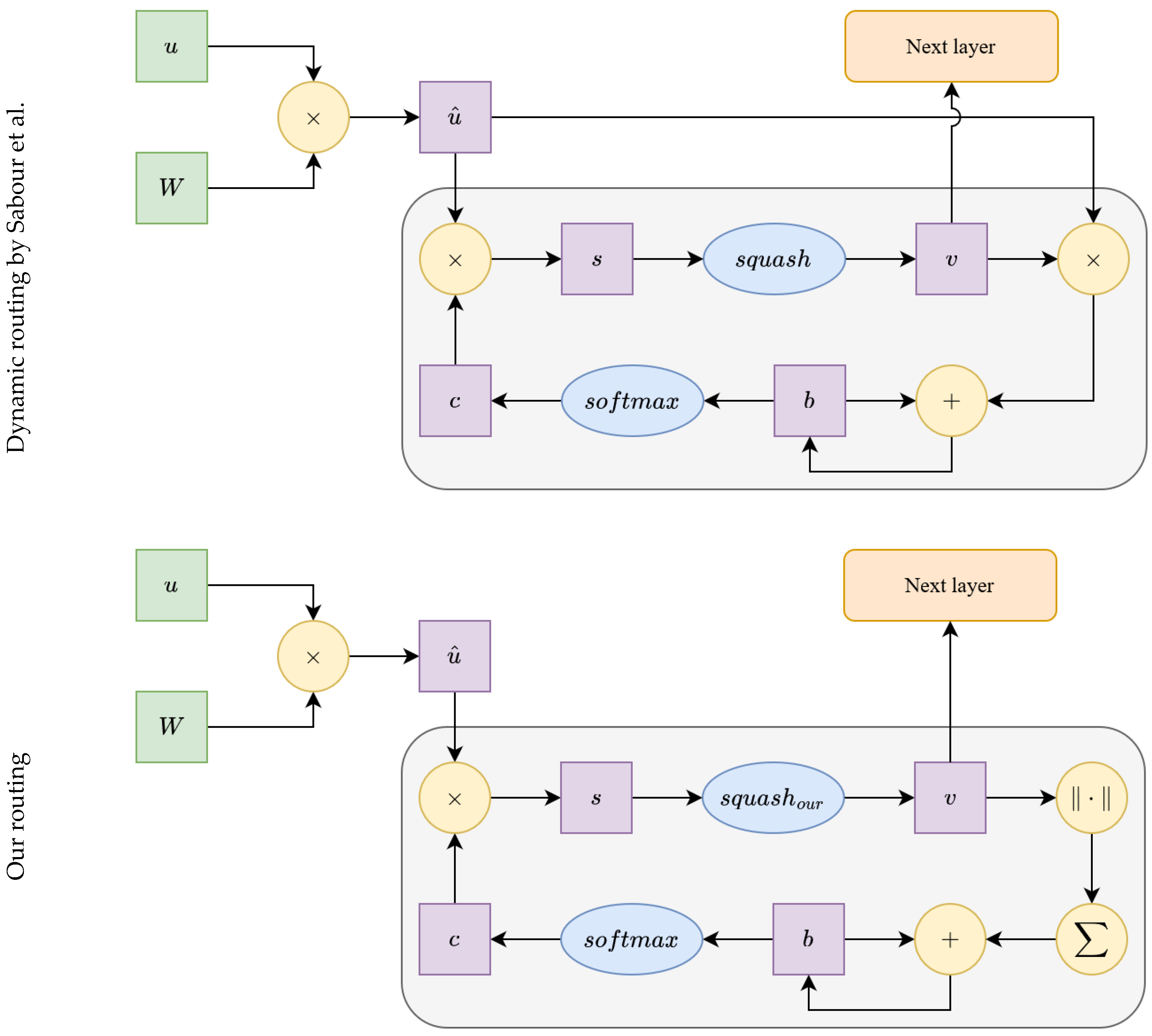
This modification simplifies the routing algorithm and improves its computational speed, as we have previously demonstrated [53,56]. Another proposed change pertains to the squashing function. In the secondary capsule layer (the structure in Figure 1), we utilize a modified squashing function as follows:
where is a fine-tuning parameter. In this research, we used as the fine-tuning parameter based on our experience. The two routing algorithms are shown in Figure 1, where the differences between the two solutions can be clearly seen.
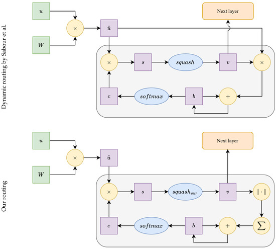
Figure 1.
Differences between the two routing mechanisms used (top: Sabour et al. [54], bottom: our proposed method).
2.3. Dataset
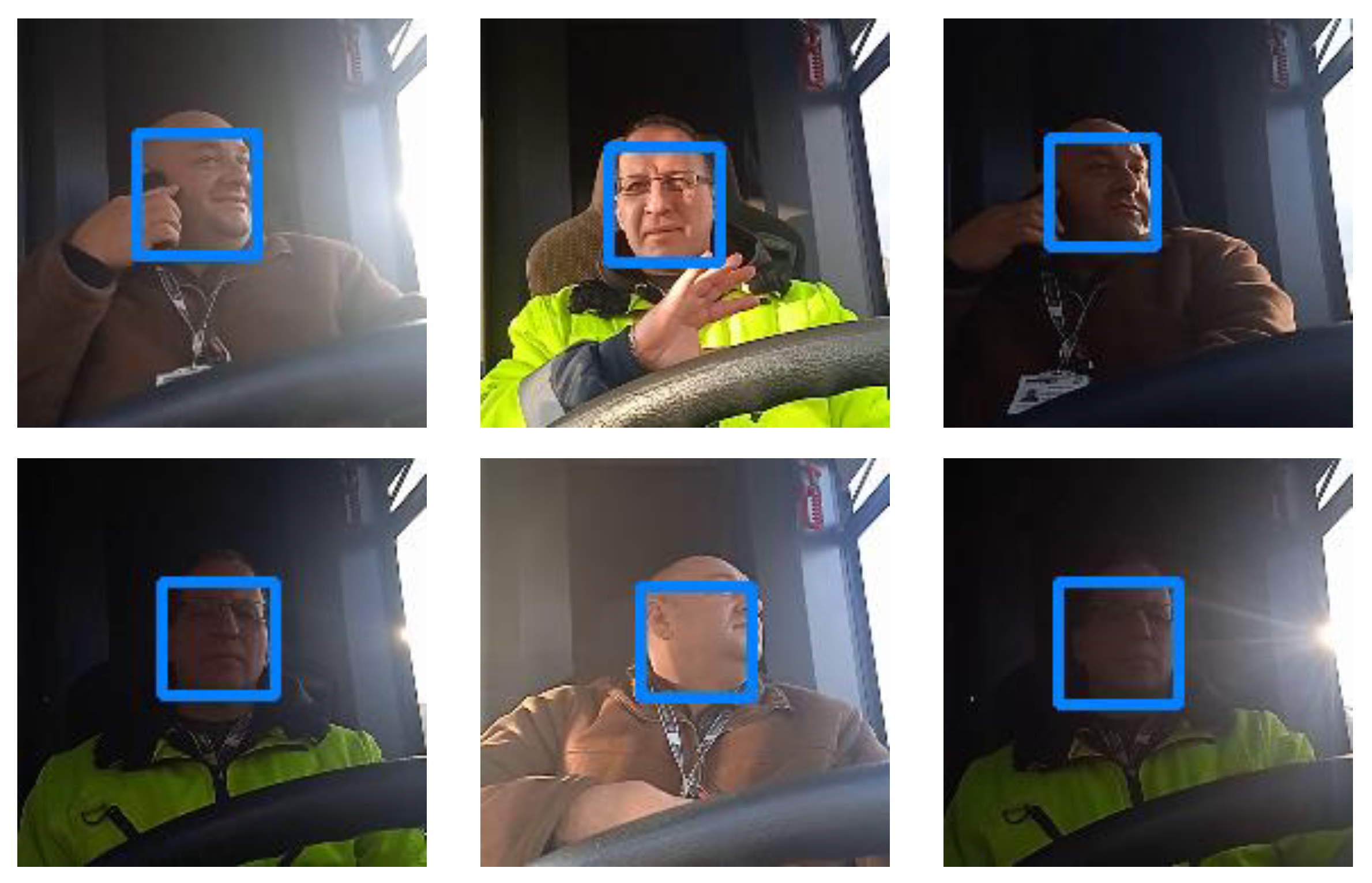
Our research aims to investigate how effectively we can detect a bus driver’s face on board a vehicle under different environmental conditions. We generated our own dataset of bus drivers in real environments and real situations. Figure 2 shows some sample images from our dataset. It was important that the dataset was as diverse as possible. Therefore, the dataset contains not only ideal samples but also various extreme but real-life scenarios. Examples include the following cases: making phone calls while driving, being in excessively shady and dark areas, and being in strong sunlight. It is crucial that the driver of the vehicle is clearly identifiable in all cases. Figure 3 shows examples of some extreme cases.
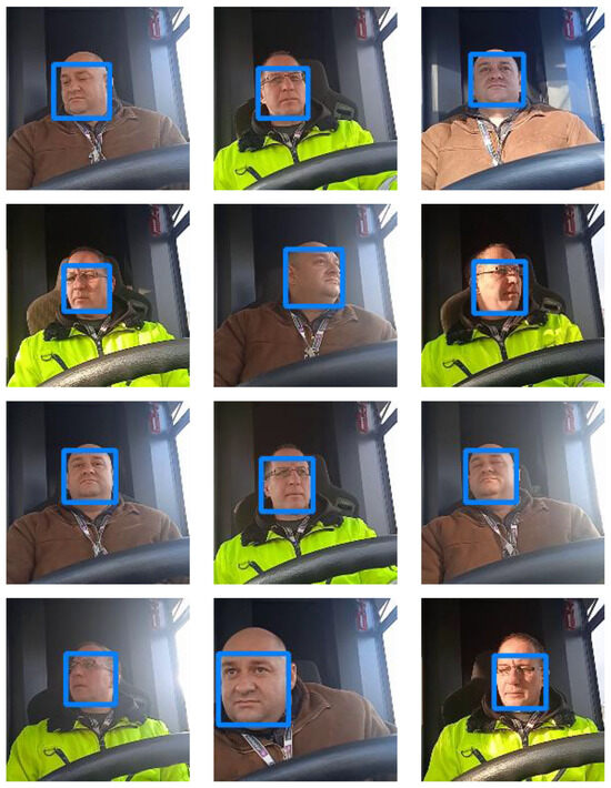
Figure 2.
Samples from our custom bus driver dataset.

Figure 3.
Some examples of extreme cases from our dataset.
Our custom dataset thus constructed contains a total of 2921 samples which are grouped into a training and test sets. The training set contains 2336 images, while the test set consists of 585 samples. All images in our dataset are 180 pixels wide by 180 pixels high and have three color channels in the RGB color space. The images were taken from a fixed camera position and depict two bus drivers with different physical characteristics.
2.4. Network Architectures
In this research, four different neural network architectures were developed. We used two different CNN architectures for a backbone. In the first case, we created an explicitly simple architecture network, which we call the Simple Network. In the second case we chose a more complex solution based on the YOLOv4 network.
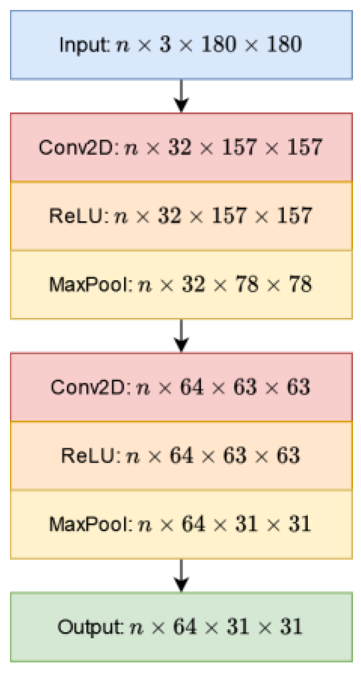
The Simple Network consists of two blocks of the following three layers: convolution, batch normalization, and max pooling. The first block contains convolution layers in size, where the maximum pooling layer kernel size is . The second block is very similar to the first, but in this case the convolution layer has outputs, where each kernel’s size is . Figure 4 shows the architecture of the Simple Network backbone.
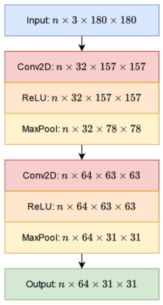
Figure 4.
Architecture of the Simple Network.
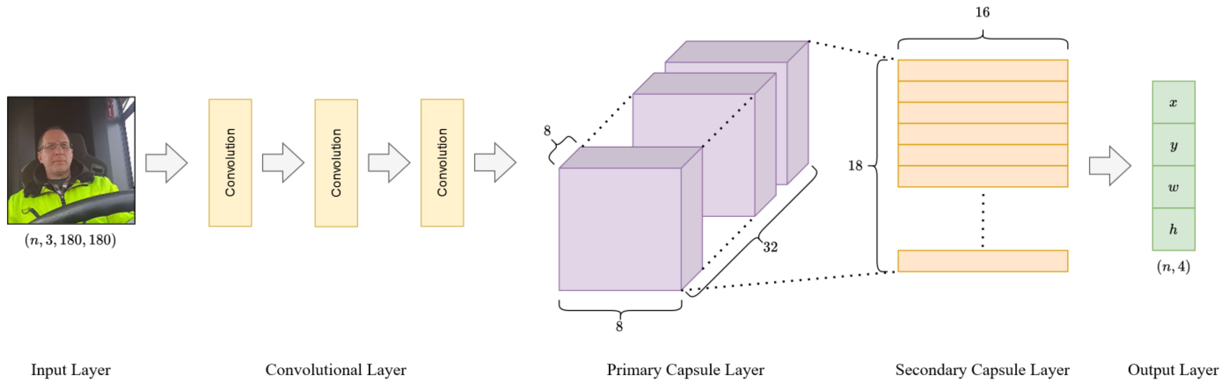
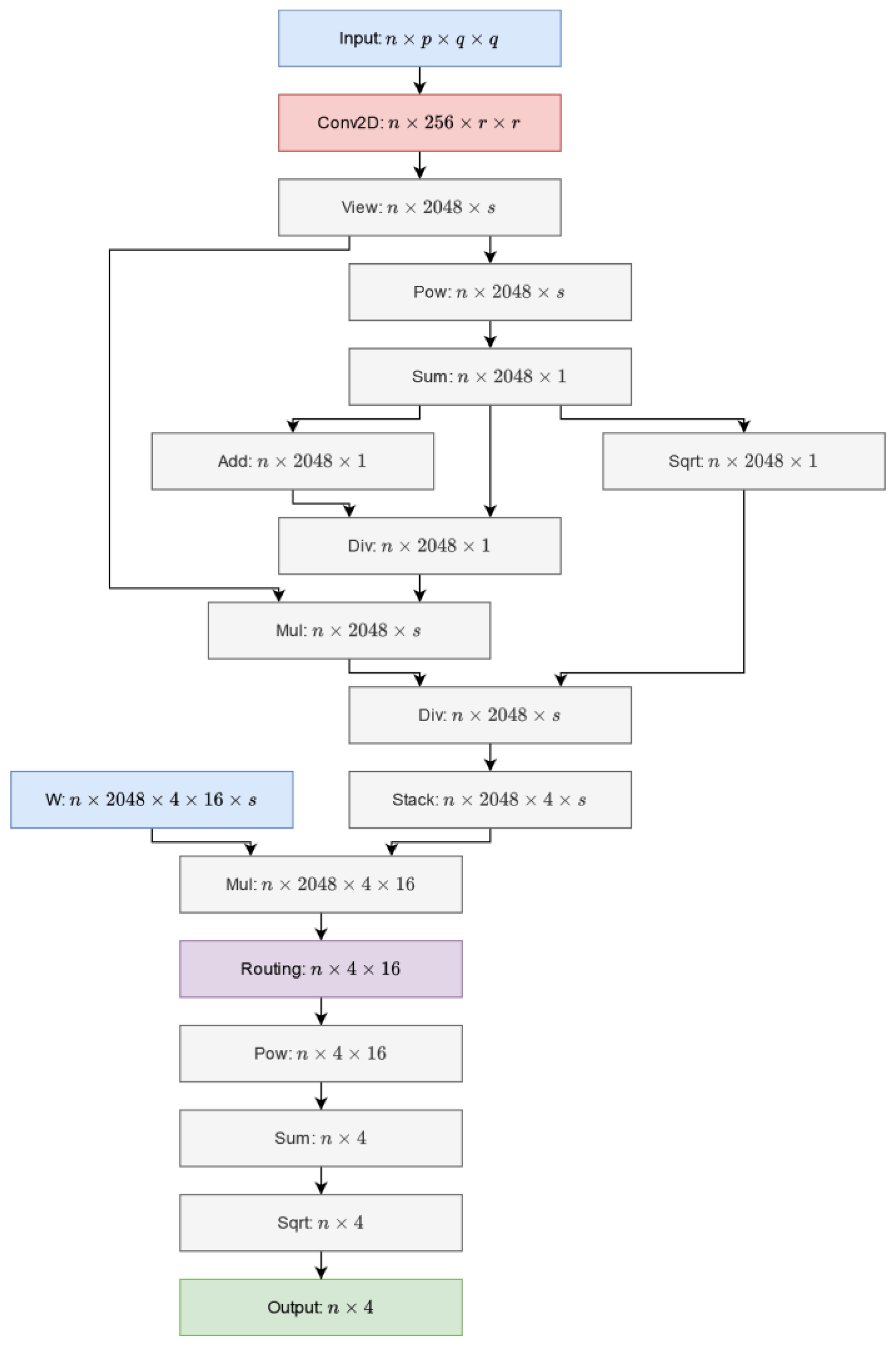
After the Simple Network we find the capsule-based subnetwork. Following the work of Sabour et al. [54], our capsule block consists of two parts: a primary capsule layer and a secondary capsule layer. In the primary capsule layer, the capsules are arranged in blocks in size, where each capsule is -dimensional. At the output of the secondary capsule layer, there are only 4 capsules, each with dimensions. Based on the capsules’ lengths, the final output quartet is generated; this contains the central coordinate, the width and the height of the bounding box. Figure 5 shows the design of our SimpleCaps network.

Figure 5.
Architecture of the SimpleCaps Network.
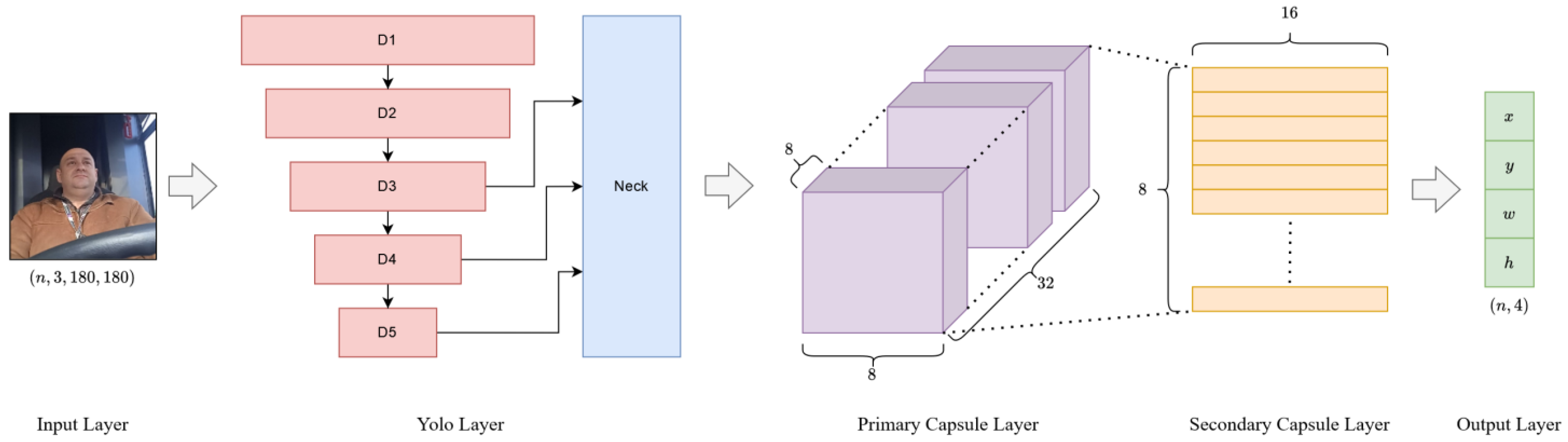
The other backbone network used in this research is modelled on YOLOv4 architecture. Its structure is illustrated in Figure 6, where our YOLOCaps network is shown. The YOLO-based backbone consists of 5 downsampling subnetworks and a neck subnetwork, where the last 3 downsampling layers (D3, D4, and D5) are used as inputs to the neck subnetwork.
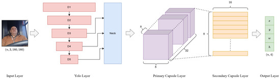
Figure 6.
Architecture of the YOLOCaps Network.
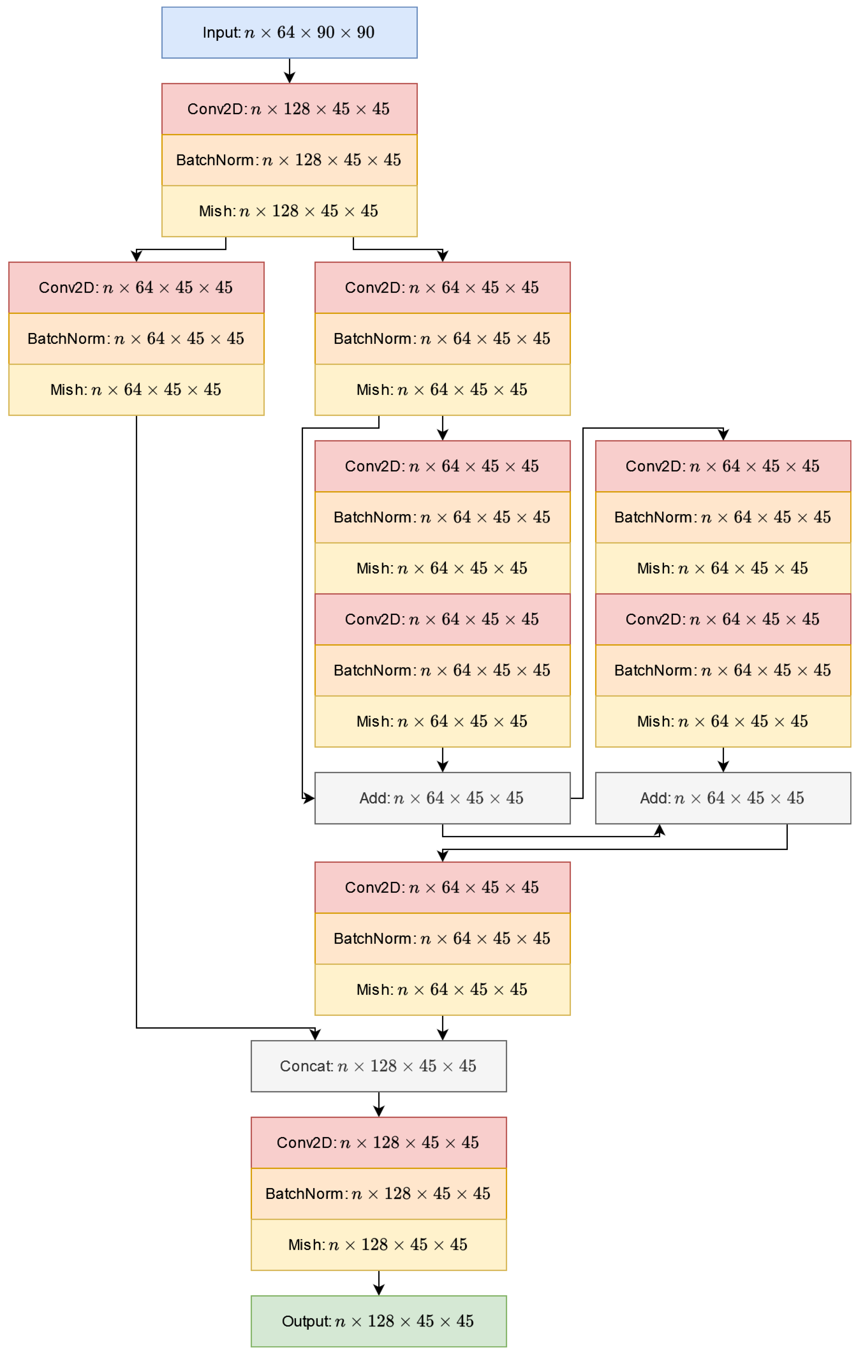
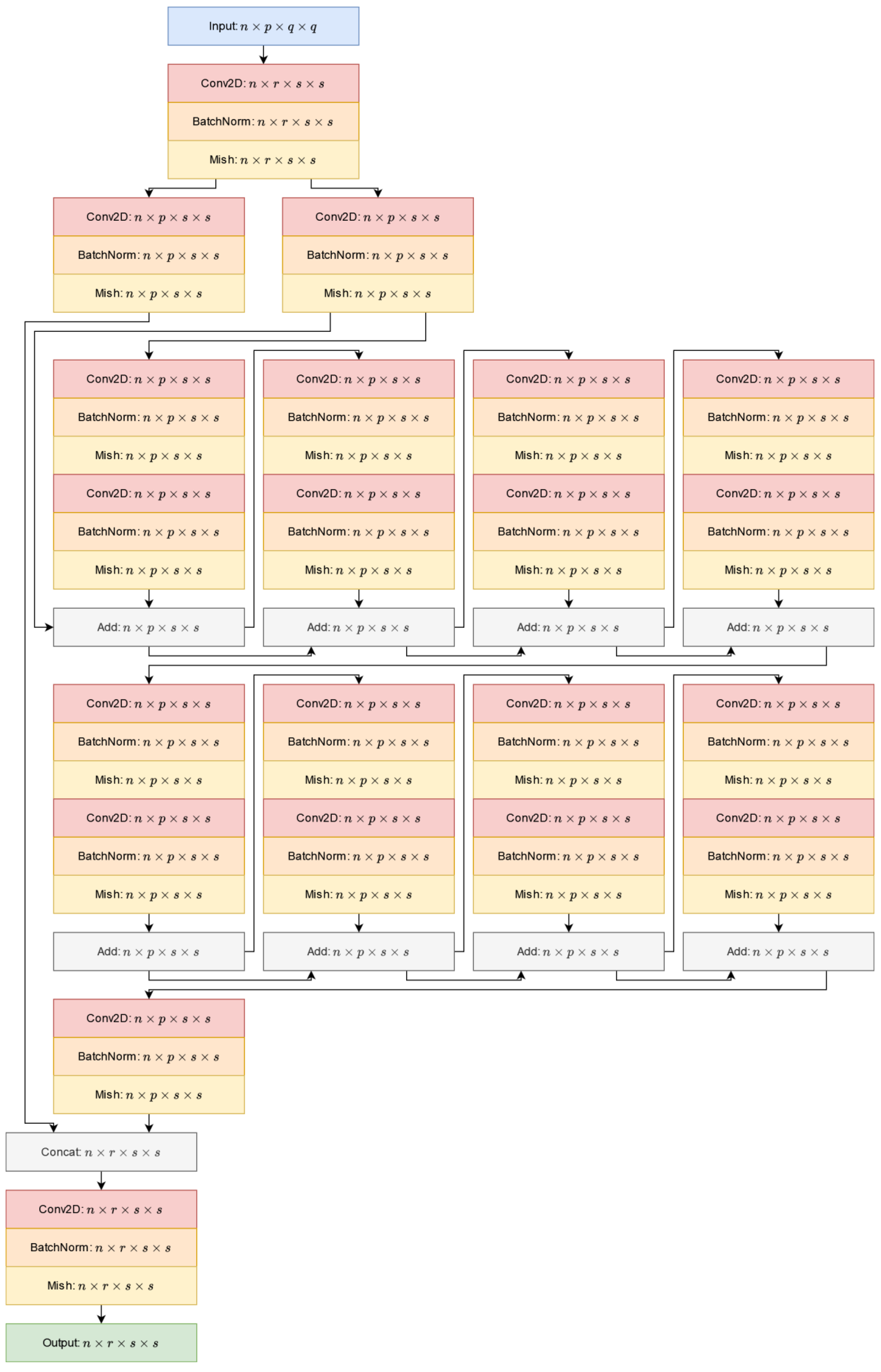
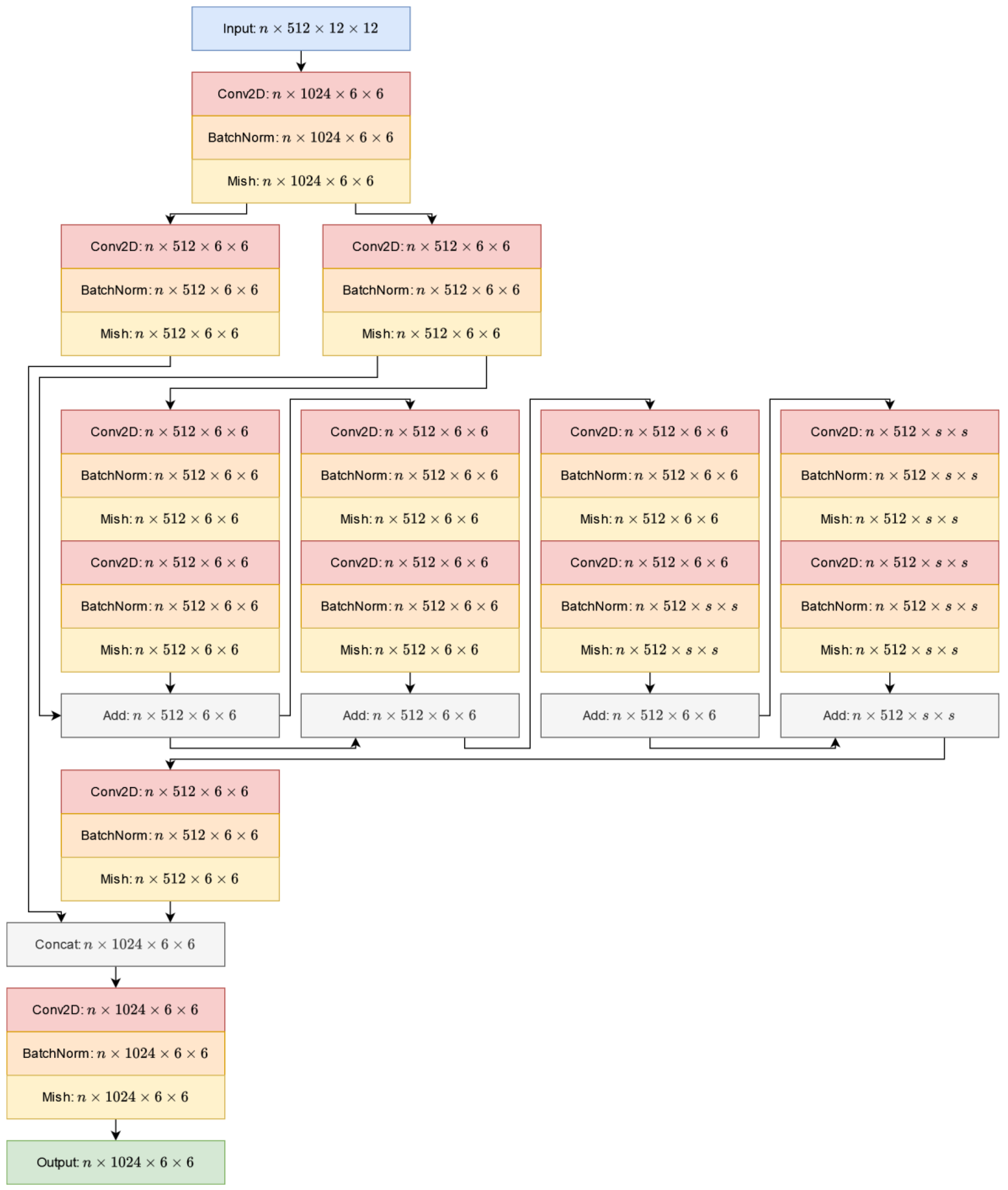
There are a total of 5 downsampling layers in the YOLO-based subnetwork, and these are called D1, D2, D3, D4, and D5. The D2, D3, D4, and D5 layers are quite similar, the only difference being the number of residual blocks; each residual block consists of two convolutional blocks, which means the following 3 layers: single 2D convolution, batch normalization, and Mish activation. The D2 layer contains 2 residual blocks. Downsampling layers D3 and D4 are made up of 8 residual blocks. Finally, in the D5 layer, only 4 residual blocks are observed. Figure 7, Figure 8, Figure 9 and Figure 10 illustrate the structures of these 5 downsampling layers, and for each figure, is the batch size. Figure 9 shows the structures of layers D3 and D4. The architecture of these two layers is identical, the only differences being the following parameters. For the D3 downsampling layer, , , , and . For the D4 downsampling layer, , , , and .
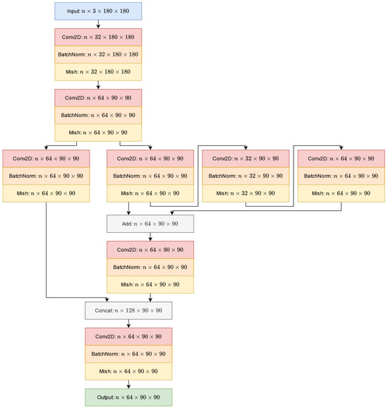
Figure 7.
Architecture of the D1 layer.
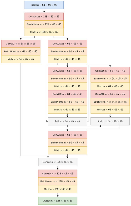
Figure 8.
Architecture of the D2 layer.
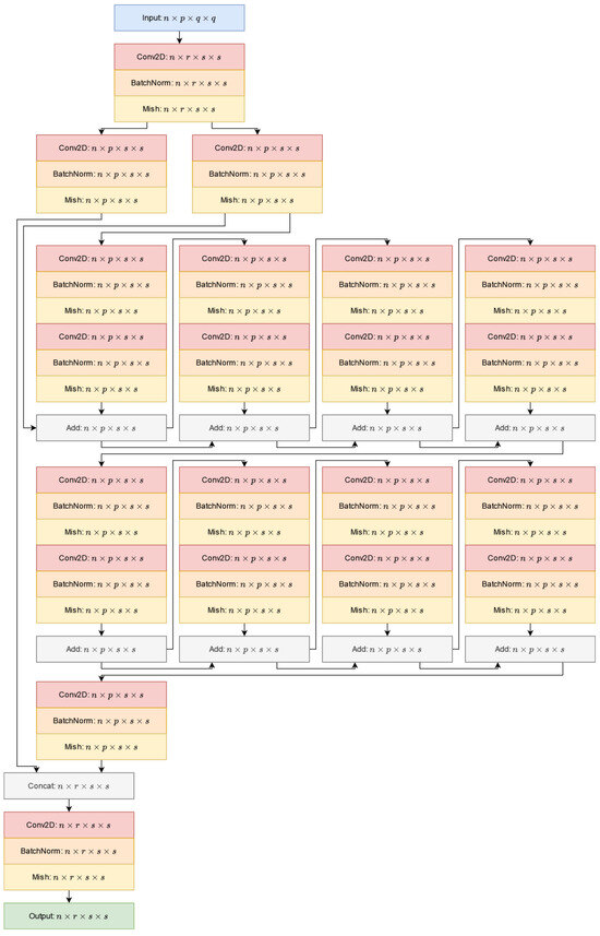
Figure 9.
Architecture of the D3 and D4 layers.
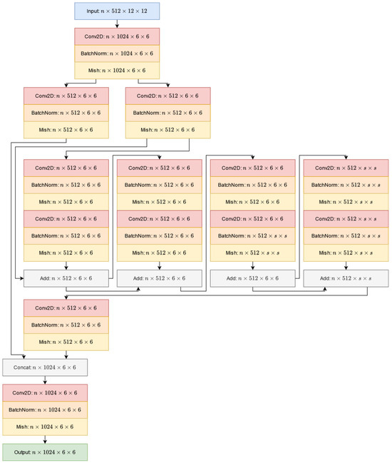
Figure 10.
Architecture of the D5 layer.
There are outputs from the downsampling layer which serve as inputs to the neck layer. These are the outputs of layers D3, D4, and D5. In the neck subnetwork, the inputs pass through different convolutional layers. The upsampling layer uses interpolation to increase the size. The structure of the neck layer is shown in Figure 11. In the neck layer, the convolutional block is a little different from that in the downsampling layers. In this case the activation function is a leaky ReLU [57].
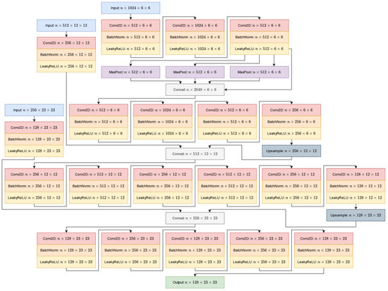
Figure 11.
Architecture of the neck layer.
The capsule-based solution is now also at the end of the network. The architecture is the same as for the SimpleCaps Network, only the number of dimensions of the capsules in the primary layer changes. In this case, the capsule’s length is .
The capsule layer structure used for the SimpleCaps and YoloCaps networks is shown in Figure 12. Different parameters were used for the two solutions. For the SimpleCaps network, , , , and . For the YoloCaps network, , , , and .
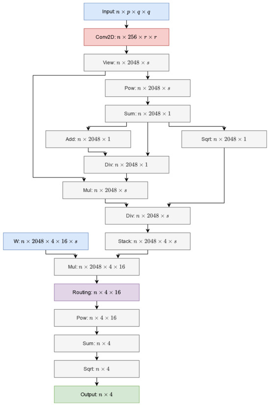
Figure 12.
Architecture of the capsule layer.
SimpleCaps and YOLOCaps networks have been implemented in two ways. In one case, the routing algorithm of Sabour et al. [54] was applied, and in the other case, our proposed method was used for routing. In this way, the two optimization algorithms can be compared under different conditions.
3. Training and Results
In the following, the main parameters of the training of the designed networks are presented. During the training process, four networks were taught under the same conditions: SimpleCaps (with our routing), SimpleCaps (with Sabour et al.’s routing), YOLOCaps (with our routing), and YOLOCaps (with Sabour et al.’s routing). The optimization was performed using the Adam [58] optimization algorithm. We set the initial learning rate to , which is an ideal initial value based on our empirical experience. We used the learning decay technique, where the exponential decay is . In this research, a smooth L1 loss function was used with the following formula:
where is the loss for the -th sample, is the ground truth for the -th sample, and is the predicted bounding box for the -th sample. We used batches in size for both training and testing. The training was carried out in epochs. Our experience has shown that after epochs, there is no significant change in the learning curve of any implemented network.
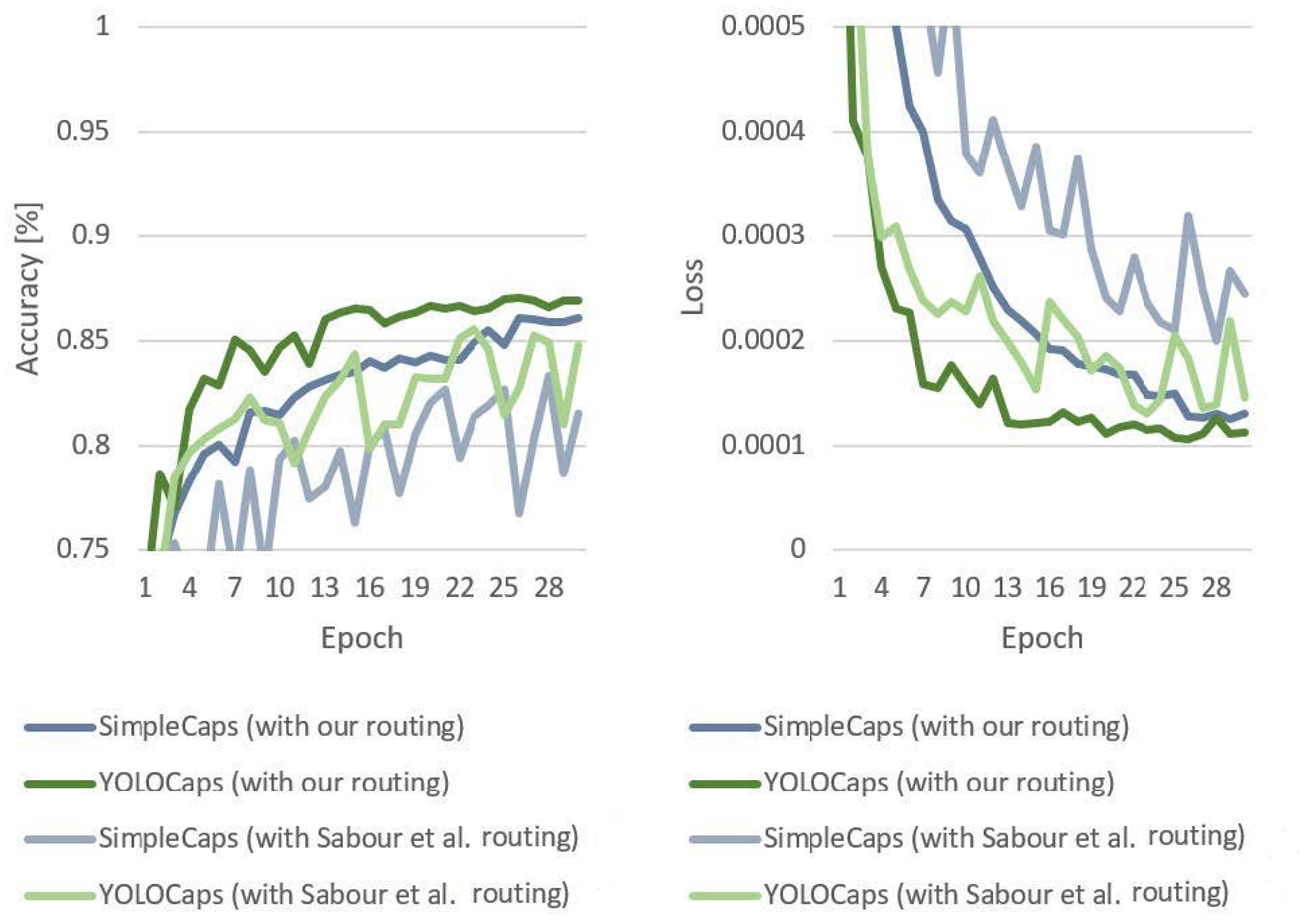
The IoU metric, which gives the ratio of the intercept and union of the ground truth and predicted rectangles, was used to measure efficiency. Figure 13 (left side) shows the learning curves under the training process for the four different networks. The best efficiency was achieved by using the YOLOCaps network with our proposed optimization routing algorithm. One might expect the second-best result to be achieved by the other YOLOCaps network, but this was not the case. The SimpleCaps Network used with our own routing algorithm was able to achieve better results than this. In third place was the YOLOCaps network, based on the algorithm by Sabour et al., while the last network in the ranking was the SimpleCaps network based on Sabour et al.’s solution.
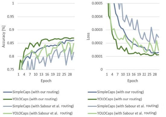
Figure 13.
Accuracy and loss measured using the test set during the training process (in some details on the basis of [54]).
Figure 13 (right side) shows the loss measured on the test set during training. Here, we can see a similar pattern to that observed when measuring accuracy. Again, the networks using our proposed optimization algorithm performed best. The lowest loss was achieved with the YOLOCaps network, followed by the SimpleCaps network. This was followed by the networks that used the solutions proposed by Sabour et al. (again, YOLOCaps followd by SimpleCaps).
Table 3 presents a summary of the results obtained in this research. Accuracy was measured using the intersection over union metric, while speed was measured by the training time of one epoch. For the SimpleCaps networks, the capsule-based subnetwork had 1,327,360 parameters, while for the YOLOCaps networks, the number of parameters was 2,654,464. The numerical results indicate that the proposed routing optimization algorithm achieves better results in both cases. Additionally, our solution was not only more efficient, but also faster. It is worth noting that in the case of SimpleCaps, our solution outperformed Sabour et al.’s solution in the case of YOLOCaps.
Table 3.
Results of the different network architectures.
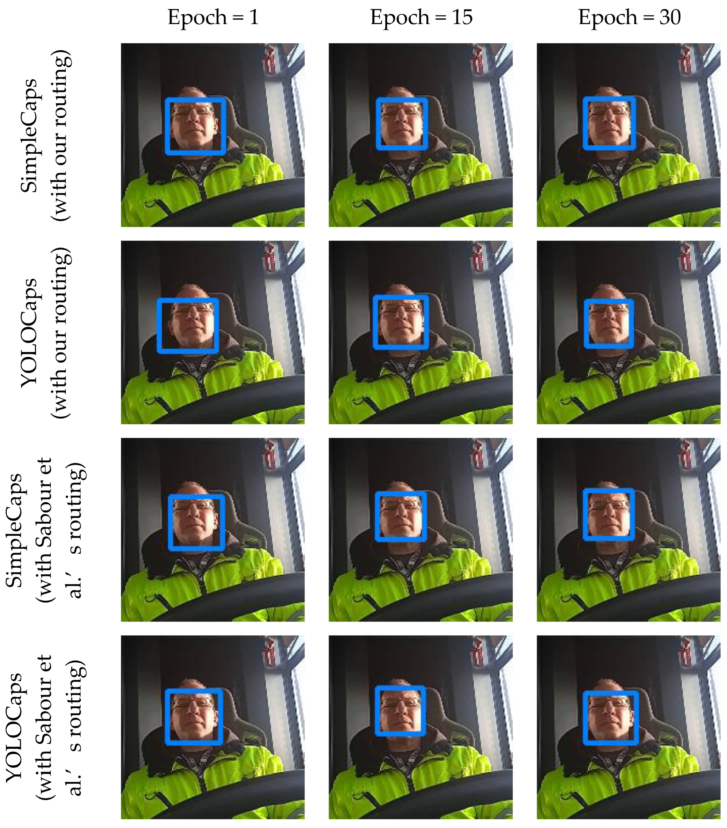
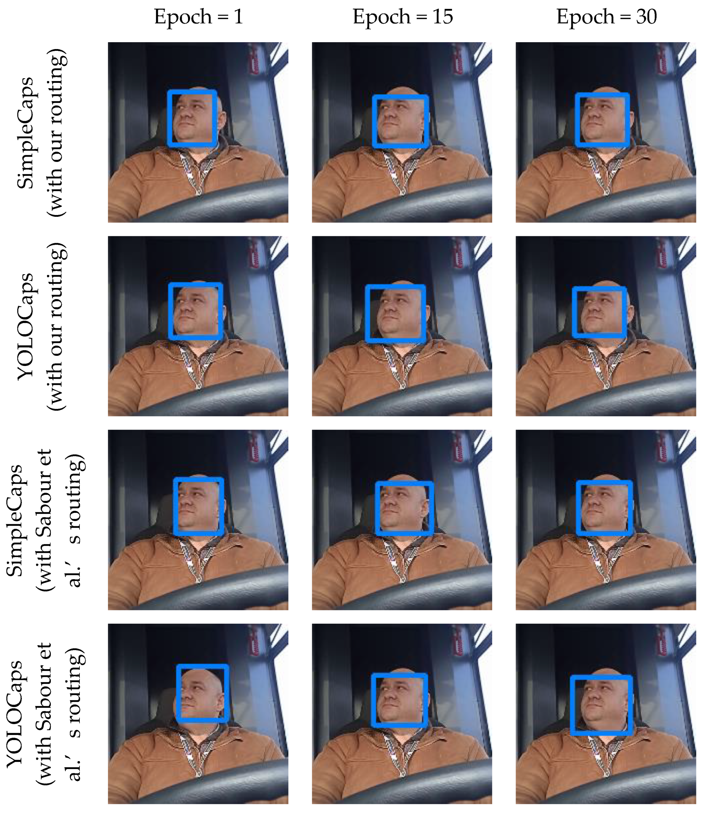
Figure 14 and Figure 15 illustrate the effectiveness of each solution for a sample image. The results for epochs 1, 15, and 30 are presented. Despite the differences, all the solutions are highly efficient; however, subtle differences can be seen between the solutions.

Figure 14.
Visualizing efficiency at different stages of the training process #1 (in some details on the basis of [54]).

Figure 15.
Visualizing efficiency at different stages of the training process #2 (in some details on the basis of [54]).
4. Discussion
This research introduces four innovative solutions for an image-based DMS, focusing on architecture and data processing techniques. These include the following: A simple network backbone featuring a dual-block design, each block comprising a convolution layer, batch normalization, and max pooling, intended for efficient feature processing. A YOLO-based backbone, which utilizes a YOLO framework with five downsampling layers, the last three of which serve as inputs to a ‘neck’ subnetwork, enhancing feature extraction capabilities. SimpleCaps and YOLOCaps networks were implemented with two routing strategies: Sabour et al.’s methodology and the novel routing approach we developed. Both networks use a downsampling layer consisting of a convolution layer, batch normalization, and an activation layer sequence. These solutions explore different configurations and routing algorithms to identify the most effective system for real-time driver monitoring and public transportation safety.
From the standpoint of its application, particularly in the context of enhancing safety within public transportation systems, a paramount consideration for an image-based DMS is the necessity for solutions that are both highly efficient and robust. The integrity of data capture is significantly influenced by external variables, including vibrations, camera lens contamination, variability in lighting conditions, and other factors that may degrade optical performance or result in occlusions. Notably, our implementation, referred to as SimpleCaps, surpassed the performance metrics of the YOLOCaps solution proposed by Sabour et al. The innovation introduced herein not only exhibits increased efficiency but also enhances processing speed, indicating significant prospects for further advancements.
This research aims to broaden the exploration of these algorithms’ practical applicability and to propose a modular system design for easy implementation. Essential requirements for on-board DMSs encompass the ability for high-speed, real-time data processing, minimal power consumption, adaptable connectivity, and comprehensive robustness across both software and hardware components.
However, our research also acknowledges certain limitations. The performance of our proposed solutions can be significantly affected by operational environmental factors, such as vibrations, lens contamination, and variable lighting conditions. Despite the demonstrated improvements in efficiency and robustness, there remains a need for further optimization to strike an optimal balance between real-time data processing speed, power consumption, and connectivity.
Looking ahead, future research will concentrate on overcoming these limitations. Efforts will be directed towards enhancing environmental robustness through the development of more sophisticated algorithms and hardware solutions. Additionally, there is a need to refine system components to improve power efficiency, connectivity, and processing speed, making the DMS more practical for real-world applications. Exploring the potential applicability of these solutions in areas beyond public transportation, including personal vehicle safety and autonomous driving technologies, also presents a promising avenue for future work.
In sum, our research not only expands the exploration of the practical applicability of algorithms in image-based DMSs, but it also proposes a modular system design for straightforward implementation. The ultimate goal is to refine these systems into an efficient and reliable DMS that fits within a comprehensive driver monitoring framework, thereby contributing to significant advancements in public transportation safety.
5. Conclusions
In this work, a comparative analysis of two distinct network designs—SimpleCaps and YOLOCaps—was conducted. Each network was integrated with a capsule-based layer and assessed using differing routing algorithms, including a novel optimization technique developed by the authors and a method proposed by Sabour et al. Our findings unequivocally demonstrate that the proposed routing algorithm outperforms the existing solution in terms of accuracy across all tested scenarios. Crucially, the simpler network architecture (SimpleCaps) not only achieved superior performance over the more complex YOLOCaps network, but it also benefitted from reduced training durations.
This outcome underscores the effectiveness of our proposed routing mechanism, particularly in enhancing the performance of less complex network designs. It also suggests the potential for significant improvements in training time, which is a critical factor in developing and deploying DMS technologies. The implications of these findings are profound, offering a promising avenue for future research and practical applications in driver monitoring systems, especially within the context of public transportation safety. Our algorithm is crucial for advancing safety systems, reducing fatigue-related risks for truck drivers, and enhancing public transport safety for trams and trains, thereby showcasing the broad applicability of our approach and its impact on transportation safety.
Author Contributions
Conceptualization, J.H. and V.N.; methodology, J.H. and V.N.; software, J.H.; validation, J.H. and V.N.; formal analysis, J.H. and V.N.; investigation, J.H. and V.N.; resources, J.H. and V.N.; data curation, J.H. and V.N.; writing—original draft preparation, J.H., Á.B., G.K., S.F. and V.N.; writing—review and editing, J.H., Á.B., G.K., S.F. and V.N.; visualization, J.H.; supervision, J.H., Á.B., G.K., S.F. and V.N.; project administration, J.H., S.F. and V.N.; funding acquisition, J.H., S.F. and V.N. All authors have read and agreed to the published version of the manuscript.
Funding
This research received no specific grant from any funding agencies.
Data Availability Statement
All data used in this research are presented in the article.
Acknowledgments
The authors wish to acknowledge the support received from the Vehicle Industry Research Centre and Széchenyi István University, Győr. This research was carried out as a part of the Cooperative Doctoral Program supported by the National Research, Development and Innovation Office and Ministry of Culture and Innovation.
Conflicts of Interest
The authors declare no conflicts of interest.
References
- Blades, L.; Douglas, R.; Early, J.; Lo, C.Y.; Best, R. Advanced Driver-Assistance Systems for City Bus Applications. SAE Tech. Pap. 2020, 2020. [Google Scholar] [CrossRef]
- Eurostat Passenger Transport by Buses and Coaches by Type of Transport—Vehicles Registered in the Reporting Country. Available online: https://ec.europa.eu/eurostat/web/transport/data/database (accessed on 2 March 2024).
- Goh, K.; Currie, G.; Sarvi, M.; Logan, D. Factors Affecting the Probability of Bus Drivers Being At-Fault in Bus-Involved Accidents. Accid. Anal. Prev. 2014, 66, 20–26. [Google Scholar] [CrossRef]
- Ferreira, S.; Kokkinogenis, Z.; Couto, A. Using Real-Life Alert-Based Data to Analyse Drowsiness and Distraction of Commercial Drivers. Transp. Res. Part. F Traffic Psychol. Behav. 2019, 60, 25–36. [Google Scholar] [CrossRef]
- Young, K.; Regan, M.; Hammer, M. Driver Distraction: A Review of the Literature (Report); Monash University Accident Research Centre: Victoria, Australia, 2003; p. 66. Available online: https://citeseerx.ist.psu.edu/document?repid=rep1&type=pdf&doi=5673cc6c48ed46e3a2c83529e0961c83a3710b9a (accessed on 2 March 2024).
- Thiffault, P.; Bergeron, J. Monotony of Road Environment and Driver Fatigue: A Simulator Study. Accid. Anal. Prev. 2003, 35, 381–391. [Google Scholar] [CrossRef]
- Sahayadhas, A.; Sundaraj, K.; Murugappan, M. Detecting Driver Drowsiness Based on Sensors: A Review. Sensors 2012, 12, 16937–16953. [Google Scholar] [CrossRef] [PubMed]
- Hallac, D.; Sharang, A.; Stahlmann, R.; Lamprecht, A.; Huber, M.; Roehder, M.; Sosič, R.; Leskovec, J. Driver Identification Using Automobile Sensor Data from a Single Turn. In Proceedings of the 2016 IEEE 19th International Conference on Intelligent Transportation Systems (ITSC), Rio de Janeiro, Brazil, 1–4 November 2016; pp. 953–958. [Google Scholar] [CrossRef]
- Zhang, Z.; Tang, Y.; Zhao, S.; Zhang, X. Real-Time Surface EMG Pattern Recognition for Hand Gestures Based on Support Vector Machine. In Proceedings of the 2019 IEEE International Conference on Robotics and Biomimetics (ROBIO), Dali, China, 6–8 December 2019; pp. 1258–1262. [Google Scholar] [CrossRef]
- Campos-Ferreira, A.E.; Lozoya-Santos, J.d.J.; Tudon-Martinez, J.C.; Mendoza, R.A.R.; Vargas-Martínez, A.; Morales-Menendez, R.; Lozano, D. Vehicle and Driver Monitoring System Using on-Board and Remote Sensors. Sensors 2023, 23, 814. [Google Scholar] [CrossRef] [PubMed]
- Fischer, S.; Szürke, S.K. Detection Process of Energy Loss in Electric Railway Vehicles. Facta Univ. Ser. Mech. Eng. 2023, 21, 81–99. [Google Scholar] [CrossRef]
- Maslać, M.; Antić, B.; Lipovac, K.; Pešić, D.; Milutinović, N. Behaviours of Drivers in Serbia: Non-Professional versus Professional Drivers. Transp. Res. Part. F Traffic Psychol. Behav. 2018, 52, 101–111. [Google Scholar] [CrossRef]
- Fancello, G.; Daga, M.; Serra, P.; Fadda, P.; Pau, M.; Arippa, F.; Medda, A. An Experimental Analysis on Driving Behaviour for Professional Bus Drivers. Transp. Res. Procedia 2020, 45, 779–786. [Google Scholar] [CrossRef]
- Karimi, S.; Aghabayk, K.; Moridpour, S. Impact of Driving Style, Behaviour and Anger on Crash Involvement among Iranian Intercity Bus Drivers. IATSS Res. 2022, 46, 457–466. [Google Scholar] [CrossRef]
- Bonfati, L.V.; Mendes Junior, J.J.A.; Siqueira, H.V.; Stevan, S.L. Correlation Analysis of In-Vehicle Sensors Data and Driver Signals in Identifying Driving and Driver Behaviors. Sensors 2023, 23, 263. [Google Scholar] [CrossRef] [PubMed]
- Biondi, F.N.; Saberi, B.; Graf, F.; Cort, J.; Pillai, P.; Balasingam, B. Distracted Worker: Using Pupil Size and Blink Rate to Detect Cognitive Load during Manufacturing Tasks. Appl. Ergon. 2023, 106, 103867. [Google Scholar] [CrossRef] [PubMed]
- Underwood, G.; Chapman, P.; Brocklehurst, N.; Underwood, J.; Crundall, D. Visual Attention While Driving: Sequences of Eye Fixations Made by Experienced and Novice Drivers. Ergonomics 2003, 46, 629–646. [Google Scholar] [CrossRef] [PubMed]
- Nagy, V.; Kovács, G.; Földesi, P.; Kurhan, D.; Sysyn, M.; Szalai, S.; Fischer, S. Testing Road Vehicle User Interfaces Concerning the Driver’s Cognitive Load. Infrastructures 2023, 8, 49. [Google Scholar] [CrossRef]
- Sigari, M.-H.; Pourshahabi, M.-R.; Soryani, M.; Fathy, M. A Review on Driver Face Monitoring Systems for Fatigue and Distraction Detection. Int. J. Adv. Sci. Technol. 2014, 64, 73–100. [Google Scholar] [CrossRef]
- Biondi, F.; Coleman, J.R.; Cooper, J.M.; Strayer, D.L. Average Heart Rate for Driver Monitoring Systems. Int. J. Hum. Factors Ergon. 2016, 4, 282–291. [Google Scholar] [CrossRef]
- Fujiwara, K.; Abe, E.; Kamata, K.; Nakayama, C.; Suzuki, Y.; Yamakawa, T.; Hiraoka, T.; Kano, M.; Sumi, Y.; Masuda, F.; et al. Heart Rate Variability-Based Driver Drowsiness Detection and Its Validation With EEG. IEEE Trans. Biomed. Eng. 2019, 66, 1769–1778. [Google Scholar] [CrossRef] [PubMed]
- Dehzangi, O.; Rajendra, V.; Taherisadr, M. Wearable Driver Distraction Identification On-the-Road via Continuous Decomposition of Galvanic Skin Responses. Sensors 2018, 18, 503. [Google Scholar] [CrossRef]
- Balam, V.P.; Chinara, S. Development of Single-Channel Electroencephalography Signal Analysis Model for Real-Time Drowsiness Detection: SEEGDD. Phys. Eng. Sci. Med. 2021, 44, 713–726. [Google Scholar] [CrossRef]
- Rahman, N.A.A.; Mustafa, M.; Sulaiman, N.; Samad, R.; Abdullah, N.R.H. EMG Signal Segmentation to Predict Driver’s Vigilance State. Lect. Notes Mech. Eng. 2022, 29–42. [Google Scholar] [CrossRef]
- European Parliament Regulation (EU) 2019/2144 of the European Parliament and of the Council. Off. J. Eur. Union 2019. Available online: https://eur-lex.europa.eu/eli/reg/2019/2144/oj (accessed on 2 March 2024).
- Koay, H.V.; Chuah, J.H.; Chow, C.O.; Chang, Y.L. Detecting and Recognizing Driver Distraction through Various Data Modality Using Machine Learning: A Review, Recent Advances, Simplified Framework and Open Challenges (2014–2021). Eng. Appl. Artif. Intell. 2022, 115, 105309. [Google Scholar] [CrossRef]
- Chaves, D.; Fidalgo, E.; Alegre, E.; Alaiz-Rodríguez, R.; Jáñez-Martino, F.; Azzopardi, G. Assessment and Estimation of Face Detection Performance Based on Deep Learning for Forensic Applications. Sensors 2020, 20, 4491. [Google Scholar] [CrossRef] [PubMed]
- Safarov, F.; Akhmedov, F.; Abdusalomov, A.B.; Nasimov, R.; Cho, Y.I. Real-Time Deep Learning-Based Drowsiness Detection: Leveraging Computer-Vision and Eye-Blink Analyses for Enhanced Road Safety. Sensors 2023, 23, 6459. [Google Scholar] [CrossRef] [PubMed]
- Jain, D.K.; Jain, R.; Lan, X.; Upadhyay, Y.; Thareja, A. Driver Distraction Detection Using Capsule Network. Neural Comput. Appl. 2021, 33, 6183–6196. [Google Scholar] [CrossRef]
- Kadar, J.A.; Dewi, M.A.K.; Suryawati, E.; Heryana, A.; Zilfan, V.; Kusumo, B.S.; Yuwana, R.S.; Supianto, A.A.; Pratiwi, H.; Pardede, H.F. Distracted Driver Behavior Recognition Using Modified Capsule Networks. J. Mechatron. Electr. Power Veh. Technol. 2023, 14, 177–185. [Google Scholar] [CrossRef]
- Ren, S.; He, K.; Girshick, R.; Sun, J. Faster R-CNN: Towards Real-Time Object Detection with Region Proposal Networks. IEEE Trans. Pattern Anal. Mach. Intell. 2017, 39, 1137–1149. [Google Scholar] [CrossRef]
- Liu, T.; Stathaki, T. Faster R-CNn for Robust Pedestrian Detection Using Semantic Segmentation Network. Front. Neurorobot 2018, 12, 64. [Google Scholar] [CrossRef]
- Redmon, J.; Farhadi, A. YOLO9000: Better, Faster, Stronger. Available online: https://openaccess.thecvf.com/content_cvpr_2017/papers/Redmon_YOLO9000_Better_Faster_CVPR_2017_paper.pdf (accessed on 2 March 2024).
- Zhang, K.; Zhang, Z.; Li, Z.; Qiao, Y. Joint Face Detection and Alignment Using Multitask Cascaded Convolutional Networks. IEEE Signal Process Lett. 2016, 23, 1499–1503. [Google Scholar] [CrossRef]
- Yang, S.; Luo, P.; Loy, C.C.; Tang, X. Faceness-Net: Face Detection through Deep Facial Part Responses. IEEE Trans. Pattern Anal. Mach. Intell. 2018, 40, 1845–1859. [Google Scholar] [CrossRef]
- Chi, C.; Zhang, S.; Xing, J.; Lei, Z.; Li, S.Z.; Zou, X. Selective Refinement Network for High Performance Face Detection. 2019. Available online: https://ojs.aaai.org/index.php/AAAI/article/view/4834 (accessed on 2 March 2024).
- Deng, J.; Guo, J.; Ververas, E.; Kotsia, I.; Zafeiriou, S. RetinaFace: Single-Shot Multi-Level Face Localisation in the Wild. Available online: https://openaccess.thecvf.com/content_CVPR_2020/papers/Deng_RetinaFace_Single-Shot_Multi-Level_Face_Localisation_in_the_Wild_CVPR_2020_paper.pdf (accessed on 2 March 2024).
- Vesdapunt, N.; Cloud&ai, M.; Wang, B.; Ai, X. CRFace: Confidence Ranker for Model-Agnostic Face Detection Refinement. Available online: https://openaccess.thecvf.com/content/CVPR2021/papers/Vesdapunt_CRFace_Confidence_Ranker_for_Model-Agnostic_Face_Detection_Refinement_CVPR_2021_paper.pdf (accessed on 2 March 2024).
- Krizhevsky, A.; Sutskever, I.; Hinton, G.E. ImageNet Classification with Deep Convolutional Neural Networks. Available online: https://proceedings.neurips.cc/paper_files/paper/2012/file/c399862d3b9d6b76c8436e924a68c45b-Paper.pdf (accessed on 2 March 2024).
- Vansteenkiste, P.; Cardon, G.; Philippaerts, R.; Lenoir, M. Measuring Dwell Time Percentage from Head-Mounted Eye-Tracking Data—Comparison of a Frame-by-Frame and a Fixation-by-Fixation Analysis. Ergonomics 2015, 58, 712–721. [Google Scholar] [CrossRef]
- Goodfellow, I.J.; Shlens, J.; Szegedy, C. Explaining and Harnessing Adversarial Examples. In Proceedings of the 3rd International Conference on Learning Representations, ICLR 2015—Conference Track Proceedings, San Diego, CA, USA, 7–9 May 2015; pp. 1–11. [Google Scholar]
- He, K.; Zhang, X.; Ren, S.; Sun, J. Deep Residual Learning for Image Recognition. Available online: https://www.cv-foundation.org/openaccess/content_cvpr_2016/papers/He_Deep_Residual_Learning_CVPR_2016_paper.pdf (accessed on 2 March 2024).
- Hu, J.; Shen, L.; Sun, G. Squeeze-and-Excitation Networks. In Proceedings of the IEEE Computer Society Conference on Computer Vision and Pattern Recognition, Salt Lake City, UT, USA, 14 December 2018; pp. 7132–7141. [Google Scholar]
- Taigman, Y.; Marc’, M.Y.; Ranzato, A.; Wolf, L. DeepFace: Closing the Gap to Human-Level Performance in Face Verification. Available online: https://openaccess.thecvf.com/content_cvpr_2014/papers/Taigman_DeepFace_Closing_the_2014_CVPR_paper.pdf (accessed on 2 March 2024).
- Schroff, F.; Kalenichenko, D.; Philbin, J. FaceNet: A Unified Embedding for Face Recognition and Clustering. 2015. Available online: https://www.cv-foundation.org/openaccess/content_cvpr_2015/papers/Schroff_FaceNet_A_Unified_2015_CVPR_paper.pdf (accessed on 2 March 2024).
- Parkhi, O.M.; Vedaldi, A.; Zisserman, A. Deep Face Recognition; University of Oxford: Oxford, UK, 2015. [Google Scholar]
- Liu, W.; Wen, Y.; Yu, Z.; Li, M.; Raj, B.; Song, L. SphereFace: Deep Hypersphere Embedding for Face Recognition. 2017. Available online: https://openaccess.thecvf.com/content_cvpr_2017/papers/Liu_SphereFace_Deep_Hypersphere_CVPR_2017_paper.pdf (accessed on 2 March 2024).
- Cao, Q.; Shen, L.; Xie, W.; Parkhi, O.M.; Zisserman, A. VGGFace2: A Dataset for Recognising Faces across Pose and Age. 2017. In Proceedings of the 2018 13th IEEE International Conference on Automatic Face & Gesture Recognition (FG 2018), Xi’an, China, 15–19 May 2018. [Google Scholar]
- Duong, C.N.; Quach, K.G.; Jalata, I.; Le, N.; Luu, K. MobiFace: A Lightweight Deep Learning Face Recognition on Mobile Devices. 2018. In Proceedings of the 2019 IEEE 10th International Conference on Biometrics Theory, Applications and Systems (BTAS), Tampa, FL, USA, 23–26 September 2019. [Google Scholar]
- Verma, B.; Choudhary, A. Deep Learning Based Real-Time Driver Emotion Monitoring. In Proceedings of the 2018 IEEE International Conference on Vehicular Electronics and Safety, ICVES, Madrid, Spain, 12–14 September 2018; pp. 1–6. [Google Scholar] [CrossRef]
- Ali, S.F.; Hassan, M.T. Feature Based Techniques for a Driver’s Distraction Detection Using Supervised Learning Algorithms Based on Fixed Monocular Video Camera. KSII Trans. Internet Inf. Syst. 2018, 12, 3820–3841. [Google Scholar] [CrossRef]
- Liu, W.; Wang, X. Researches Advanced in Face Recognition. Highlights Sci. Eng. Technol. AMMSAC 2023, 49, 41. [Google Scholar] [CrossRef]
- Hollósi, J.; Ballagi, Á.; Kovács, G.; Fischer, S.; Nagy, V. Face Detection Using a Capsule Network for Driver Monitoring Application. Computers 2023, 12, 161. [Google Scholar] [CrossRef]
- Sabour, S.; Frosst, N.; Hinton, G.E. Dynamic Routing between Capsules. 2017. Available online: https://arxiv.org/pdf/1710.09829.pdf (accessed on 2 March 2024).
- Hinton, G.E.; Krizhevsky, A.; Wang, S.D. Transforming Auto-Encoders; Springer: Berlin/Heidelberg, Germany, 2014. [Google Scholar] [CrossRef]
- Hollósi, J.; Ballagi, Á.; Pozna, C.R. Simplified Routing Mechanism for Capsule Networks. Algorithms 2023, 16, 336. [Google Scholar] [CrossRef]
- Xu, B.; Wang, N.; Chen, T.; Li, M. Empirical Evaluation of Rectified Activations in Convolutional Network. arXiv 2015, arXiv:1505.00853. [Google Scholar]
- Kingma, D.P.; Ba, J. Adam: A Method for Stochastic Optimization. arXiv 2014, arXiv:1505.00853. [Google Scholar]


Disclaimer/Publisher’s Note: The statements, opinions and data contained in all publications are solely those of the individual author(s) and contributor(s) and not of MDPI and/or the editor(s). MDPI and/or the editor(s) disclaim responsibility for any injury to people or property resulting from any ideas, methods, instructions or products referred to in the content. |
© 2024 by the authors. Licensee MDPI, Basel, Switzerland. This article is an open access article distributed under the terms and conditions of the Creative Commons Attribution (CC BY) license (https://creativecommons.org/licenses/by/4.0/).