Article

Least Squares Minimum Class Variance Support Vector Machines

by
Michalis Panayides
1 and
Andreas Artemiou
2,*
1
School of Mathematics, Cardiff University, Cardiff CF24 4HQ, UK
2
Department of Information Technologies, University of Limassol, 3025 Limassol, Cyprus
*
Author to whom correspondence should be addressed.
Computers 2024, 13(2), 34; https://doi.org/10.3390/computers13020034
Submission received: 12 December 2023 / Revised: 23 January 2024 / Accepted: 24 January 2024 / Published: 26 January 2024
(This article belongs to the Special Issue Uncertainty-Aware Artificial Intelligence)

Abstract

:
In this paper, we propose a Support Vector Machine (SVM)-type algorithm, which is statistically faster among other common algorithms in the family of SVM algorithms. The new algorithm uses distributional information of each class and, therefore, combines the benefits of using the class variance in the optimization with the least squares approach, which gives an analytic solution to the minimization problem and, therefore, is computationally efficient. We demonstrate an important property of the algorithm which allows us to address the inversion of a singular matrix in the solution. We also demonstrate through real data experiments that we improve on the computational time without losing any of the accuracy when compared to previously proposed algorithms.

1. Introduction

Support Vector Machines (SVMs) have been used in a number of disciplines since their introduction by [1] for classification and regression. Although the name is used to describe the classic algorithm proposed by [1], SVMs have been extended in many different directions and a lot of authors are now using the name to refer to a family of methods that are based on the original idea by [1]. The basic purpose of SVM algorithms in binary classification is to find an optimal hyperplane which separates the two classes of datapoints with the maximum margin when the data are separable (hard margin). In cases where the classes are not separable, a soft margin approach is used which finds the optimal hyperplane by maximizing the margin and minimizing the sum of the misclassification distances of the misclassified points.
There are three features that have made SVM algorithms popular since their introduction. The first one is the use of nonlinear kernels, which map the observations from the current space into a higher dimensional feature space to achieve linear separability of the points using the kernel trick, that is without the need to know the exact mapping to the feature space. The second important aspect of SVMs is the fact that they target the minimization of structural risk (minimizing the risk of the misclassification of unseen observations) rather than the minimization of empirical risk (minimizing the risk for points in the sample). Finally, the optimization problem is solved relatively efficiently using quadratic programming.
SVMs are continuing to be a popular option for researchers looking for classification methodology to apply to their datasets. Therefore, there is a constant need for new approaches to be developed within the SVM framework in classification to address the many challenges that the new era of massive and high-dimensional datasets brings to researchers. A very small sample of new methods being proposed in the SVM literature includes [2], which proposes a new fuzzy approach to Twin SVMs; [3], which presents an improved version of the SVM with the radial basis function; and [4], who proposed a twin SVM algorithm with the pinball loss. At the same time, there are some recent works which demonstrate the usefulness in applying SVM variants for classification in other sciences. See, for example, [5] who applied SVMs to Twitter data, the work by the authors in [6] who applied SVMs to remote sensing data, and [7] who applied them in seismic data.
In this paper, we propose a computationally efficient SVM-type algorithm which uses distributional information of the classes. To achieve a computationally fast algorithm, we replace the hinge loss in the classic SVM algorithms with the least squares approach, in a similar way as it was done in the Least Squares SVM (LSSVM) by [8]. To introduce the distributional information of the classes, we propose the use of the within-class variance in a similar way as it was proposed in the Minimum Class Variance SVM (MCVSVM) by [9], who reformulated the optimization problem in Fisher’s linear discriminant analysis (LDA) to achieve this.
In Section 2, we revisit the algorithms in the literature which are important for our development and in Section 3, we propose our new algorithm, presenting both the linear and nonlinear approaches to the algorithm. We demonstrate a very powerful property of the algorithm, which can overcome the issue of finding an inverse by using principal projections, which is needed for the solution in Section 4. We discuss some real data analysis in Section 5 and we close with a discussion section.

2. Literature Review on SVMs

In this section, we review some of the algorithms in the SVM family that were useful for the development of our idea. We start with the classic SVM by [1] and then we present the Least Squares SVM approach by [8]. Finally, we discuss the Minimum Class Variance SVM (MCVSVM) by [9]. All the algorithms were initially developed in the simple case where data are separable, and then extended in the soft margin case where the data are not linearly separable. In this paper, we talk about the most general approach, that is, the soft margin approach.

2.1. Support Vector Machines (SVMs)

The classic SVM algorithm was proposed by [1]. In the most general case, to find the optimal separating hyperplane, it was proposed to solve the following optimization problem:
min 1 2 ψ T ψ + λ i = 1 n ξ i
under the constraints:
y i ( ψ T x i t ) 1 ξ i , ξ i 0 ,
where ( ψ , t ) R p × R is the pair that characterizes the hyperplane that has equation ψ T X t = 0 , λ is a scalar known as the cost or the misclassification penalty, and the ξ i ’s are slack variables which denote misclassification distances. If a point is correctly classified, the slack variable ξ i associated with it is set to 0, and if the point is incorrectly classified, the ξ i denotes the distance of the variable to the to the hyperplane.
To find the solution to the optimization problem above, one uses the Lagrangian multipliers and tries to minimize the following Lagrangian equation:
L ( ψ , t , ξ , α , β ) = 1 2 ψ T ψ + λ i = 1 n ξ i i = 1 n α i ( 1 ξ i y i ( ψ T x i t ) ) i = 1 n β i ξ i = 1 2 ψ T ψ + λ 1 T ξ α T ( 1 ξ y ( ψ T x t ) ) β T ξ
where y = ( y 1 , , y n ) T R n , x = ( x 1 , , x n ) T R p × n , 1 = ( 1 , , 1 ) T R n , t = ( t , , t ) T R n , α = ( α 1 , , α n ) T R n , β = ( β 1 , , β n ) T R n , and ξ = ( ξ 1 , , ξ n ) T R n . Using the derivatives, one finds the Karush–Kuhn–Tucker (KKT) equations:
L ψ = ψ x ( α y ) = 0 ψ = x ( α y ) , L t = α T y = 0 α T y = 0 , L ξ = λ α β = 0 .
By replacing the result of the first derivative in the Lagrangian equation, one gets:
L ( ψ , t , ξ , α , β ) = 1 2 ( x ( α y ) ) T x ( α y ) + λ 1 T ξ α T ( 1 ξ y ( ( x ( α y ) ) T x t ) ) β T ξ = 1 2 ( α y ) T x T x ( α y ) + α T 1 ( λ 1 α β ) T ξ + ( α y ) T x T x ( α y ) + t α T y .
Now, the last term is equal to 0 from the result in the second KKT equation above, and the third term is 0 by the third KKT equation. Hence, the above Lagrangian equation reduces to:
L ( α , β ) = α T 1 1 2 ( α y ) T x T x ( α y )
subject to the constraint 0 < α < λ 1 . This is known as the dual problem. One can use quadratic programming optimization to solve the dual problem to obtain α , which is essential in estimating the normal vector of the optimal hyperplane according to the solution in the first KKT equation above.
Two of the most important features of the classic SVM algorithm is the use of the hinge loss in the objective function to be minimized and the fact that, in constructing the hyperplane, only points that are incorrectly classified are used, as well as points that are closer to the hyperplane. This gives a form of sparsity to the SVM, as not all points are needed to construct the hyperplane. At the same time, it is computationally expensive as it requires the solution of a quadratic programming optimization problem.

2.2. Least Squares Support Vector Machines (LSSVMs)

A least squares approach was proposed by [8], which essentially changes the geometry of the problem from the way [1] framed it. It changes the hinge loss to the square loss, which allows one to take a least squares approach and find the solution analytically. At the same time, they changed the constraints from inequalities to equalities, allowing for the ξ i ’s to be either positive or negative, which implies that all the points are needed to find he optimal hyperplane, removing the sparsity of the classic SVM algorithm.
In the Least Squares SVM (LSSVM), one tries to find the optimal hyperplane by minimizing the following objective function:
min 1 2 ψ T ψ + λ i = 1 n ξ i 2
under the constraints:
y i ( ψ T x i t ) = 1 ξ i .
By replacing the equality constraint in the objective function, one gets that is needed to solve the objective function:
min 1 2 ψ T ψ + λ i = 1 n 1 y i ( ψ T x i t ) 2 .
To find the values of the pair ( ψ , t ) which minimizes this objective function, one needs to take the derivative with respect to both parameters. Here, we rewrite the objective function by denoting r = ( ψ T , t ) T and reexpress the above as:
r T I p , 1 r + λ i = 1 n 1 y i ( r T x i ) 2
where x i = ( x i T , 1 ) and I p , q is the ( p + q ) × ( p + q ) diagonal matrix which has 1 on the first p diagonal elements and 0 on the last q diagonal elements. In matrix form, we can write this as:
r T I p , 1 r + λ ( 1 n D Y X r ) T ( 1 n D Y X r )
where X = ( X , 1 n ) is the n × ( p + 1 ) matrix which contains the variables X and an extra column of 1 ’s, and D Y is the diagonal matrix that has the vector Y = ( Y 1 , , Y n ) on the diagonal. Taking the derivative we have:
2 I p , 1 r 2 λ X T D Y ( 1 n D Y X r )
which, if we set it to equal 0, gives the solution:
r = I p , 1 λ + ( X ) T X 1 X T D Y 1 n
where we use the fact that D Y D Y = I n , the n × n identity matrix, to simplify the notation. We are mostly interested in ψ = [ r ] p where [ · ] p denotes the first p entries in a vector or the first p rows of a matrix, depending on the type of argument being used.
As one can see from the developments in this section, LSSVM does not need quadratic optimization as it has an analytic solution and it is therefore much faster to find the equation of the optimal hyperplane.

2.3. Minimum Class Variances Support Vector Machines (MCVSVMs)

A different extension of the SVM algorithm was proposed by [9], which is called Minimum Class Variance SVM (MCVSVM). As its name suggest, this algorithm is focused on finding the optimal hyperplane, not only by maximizing the margin, but also by minimizing the class variance when projected on the normal vector. This method was inspired by Fisher’s linear discriminant analysis [10], as it uses information from the distribution of the classes to achieve better classification results. It is also interesting that the authors showed that their approach can be used in a large p small n setting, despite using the inverse of the pooled class covariance matrix (which is not invertible in large p small n settings) in their solution.
In the Minimum Class Variance SVM (MCVSVM), one tries to find the optimal hyperplane by minimizing the following objective function:
min 1 2 ψ T Σ w ψ + λ i = 1 n ξ i
under the constraints:
y i ( ψ T x i t ) 1 ξ i , ξ i 0
where Σ w is the pooled covariance matrix as a weighted average of the covariance matrices of the classes.
Using the KKT equations, the solution of the hyperplane is found using:
ψ = Σ w 1 x ( α y )

3. New Method: LS-MCVSVM

As we said in the introduction, our objective in this section is to introduce the Least Squares extension of the MCVSVM algorithm. This will allow us to utilize the advantages of both algorithms in an effort to create a much broader algorithm than the already existing one. First of all, the new algorithm is computationally very fast as it does not need quadratic optimization due to the use of the least squares approach to the MCVSVM algorithm. It is also an algorithm that utilizes the variability within each class due to the the use of the MCVSVM.
Therefore, the new algorithm minimizes the following objective function:
min 1 2 ψ T Σ w ψ + λ i = 1 n ξ i 2
under the equality constraints:
y i ( ψ T x i t ) = 1 ξ i ,
Using a similar approach as the LSSVM which we described in the review in the previous section, we replace the equality constraint in the objective function to get the new objective functions:
min 1 2 ψ T Σ w ψ + λ i = 1 n 1 y i ( ψ T x i t ) 2
We set r = ( ψ T , t ) T and we rewrite the optimization function as:
r T r + λ i = 1 n 1 y i ( r T x i ) 2
where Σ w = diag ( Σ w , 0 ) a ( p + 1 ) × ( p + 1 ) matrix and x i = ( x i T , 1 ) . We can also write this in matrix form as:
r T Σ w r + λ ( 1 n D Y X r ) T ( 1 n D Y X r )
where X = ( X , 1 n ) is the n × ( p + 1 ) matrix which contains the variables X and an extra column of 1 ’s, and D Y is the diagonal matrix that has the vector Y = ( Y 1 , , Y n ) on the diagonal. Now, if one takes the derivative and set it equal to 0, the solution is as follows:
r = Σ w λ + ( X ) T X 1 X T D Y 1 n
where, as before, r = ( ψ T , t ) T and Σ w is a ( p + 1 ) × ( p + 1 ) matrix which has Σ w in the first p × p submatrix and everything else is completed with zeroes. We omitted the details of the development as it is very similar to the one described in the LSSVM above.
It is also important to note that there are similar developments in the nonlinear setting. Let ϕ be a functions such that ϕ : R p R q where q > > p is the dimension of the feature space where the points are mapped to be separated linearly. Then, we can define the within sample variance in the Σ w Φ in the feature space as:
Σ w Φ = x C ( ϕ ( x ) μ C Φ ) ( ϕ ( x ) μ C Φ ) T + x C + ( ϕ ( x ) μ C + Φ ) ( ϕ ( x ) μ C + Φ ) T
where C , C + denote the points in each class and μ C Φ , μ C + Φ the means of the predictor vectors when transformed by ϕ to the feature space.
This means that the optimization problem we are solving involves the minimization of the following objective function:
min 1 2 ψ Φ T Σ w Φ ψ Φ + λ i = 1 n ξ i 2
under the equality constraints:
y i ( ψ Φ T ϕ ( X i ) t Φ ) = 1 ξ i ,
which will give us the solution:
r Φ = ( Σ w Φ ) λ + ϕ ( X ) T ϕ ( X ) 1 ϕ ( X ) T D Y 1 n
where r Φ = ( ψ Φ T , t Φ ) T , ( Σ w Φ ) = diag ( Σ w Φ , 0 ) , and ϕ ( X ) = ( ϕ ( X ) T , 1 ) T .

4. Addressing Singularity Using Principal Projections

As one can see in the discussion in the previous section, in order to solve the optimization problem and find r , we need the inverse matrix of:
A = Σ w λ + ( X ) T X
which may not be invertible. In this section, we will try to address the possible singularity of this matrix and demonstrate how one can overcome this difficulty using principal projections.
We first assume that the eigenvalues of A form an orthonormal basis. Then, we can define the space A spanned by the eigenvectors corresponding to the nonzero eigenvalues of A and the space A spanned by the eigenvectors corresponding to the zero eigenvalues of A . Therefore, we can write each vector in a ( p + 1 ) -dimensional space as r = ϕ + ζ , where ϕ A and ζ A .
We also note that the optimization problem in (1) alongside the constraint in (2) can be rewritten as:
min 1 2 r T Σ w r + λ i = 1 n ξ i 2
under the equality constraints:
y i ( r T x i ) = 1 ξ i ,
and when we replace ξ i from the constraint to the optimization, the above simplifies to:
min 1 2 r T Σ w r + λ i = 1 n ( 1 y i ( r T x i ) ) 2
which, in matrix form, looks like:
min 1 2 r T Σ w + λ ( X ) T ( X ) r + λ n + 2 λ r T ( X ) T D Y 1
which can also be rewritten as:
min 1 2 r T Σ w λ + ( X ) T ( X ) r + n 2 r T ( X ) T D Y 1
where, if we replace the definition of A , we get:
min 1 2 r T A r + n 2 r T ( X ) T D Y 1 .
From this, we can see that by essentially replacing r with ϕ + ζ we have:
min 1 2 ϕ T A ϕ + ζ T A ζ + n 2 ϕ T ( X ) T D Y 1 2 ζ T ( X ) T D Y 1 .
where the term ζ T A ζ = 0 , since A ζ = 0 as ζ A .
Furthermore, it is important to note that if ζ T A ζ = 0 then, because both Σ w λ and ( X ) T ( X ) are nonnegative matrices, one can show that ζ T Σ w λ ζ = 0 and ζ T ( X ) T ( X ) ζ = 0 . From the latter, one can infer that all points x i are projected on the same point under ζ , which leads to the fact that ζ T ( X ) T = k , which makes the last term a constant which can be ignored. Therefore, the optimization problem (3) is equivalent to:
min 1 2 ϕ T A ϕ + n 2 ϕ T ( X ) T D Y 1 .
Now, this means we can solve the problem in a space isomorphic to A and, essentially, we can choose to do it on the space spanned by the eigenvectors corresponding to the nonzero eigenvalues of A . These can be found using the matrix ( p + 1 ) × d matrix P (where d is the number of nonzero eigenvalues of A ), which has for columns the eigenvectors corresponding to the nonzero eigenvalues. This means the data can be projected to the new data X = X P . Similarly, we can project ϕ to get η = P T ϕ . Therefore, we can show that the objective function (4) is equivalent to:
min 1 2 η T P T A P η + n 2 η T P T ( X ) T D Y 1 .
which simplifies to:
min 1 2 η T A η + n 2 η T ( X ) T D Y 1 .
where A = P T A P = P T Σ w λ P + P T ( X ) T X P which is a d × d matrix and is also equal to Σ w λ + ( X ) T X . That is, Σ w is the within variance when X is replaced with X . Therefore, we have a projection problem which uses the projected data X in the lower dimensional space (dimension d) only and it is equivalent to the original problem in (5). The solution of this problem is:
η = ( A ) 1 X T D Y 1 n
which uses the inverse of the A , which is nonsingular by construction.

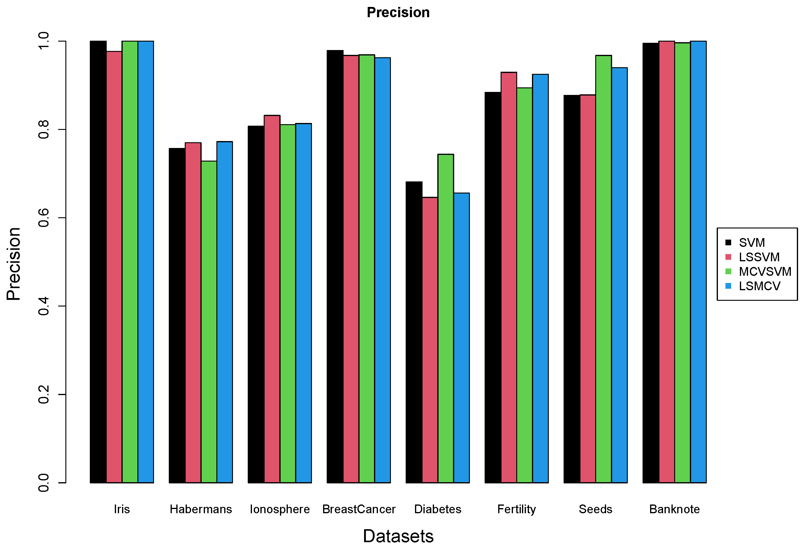
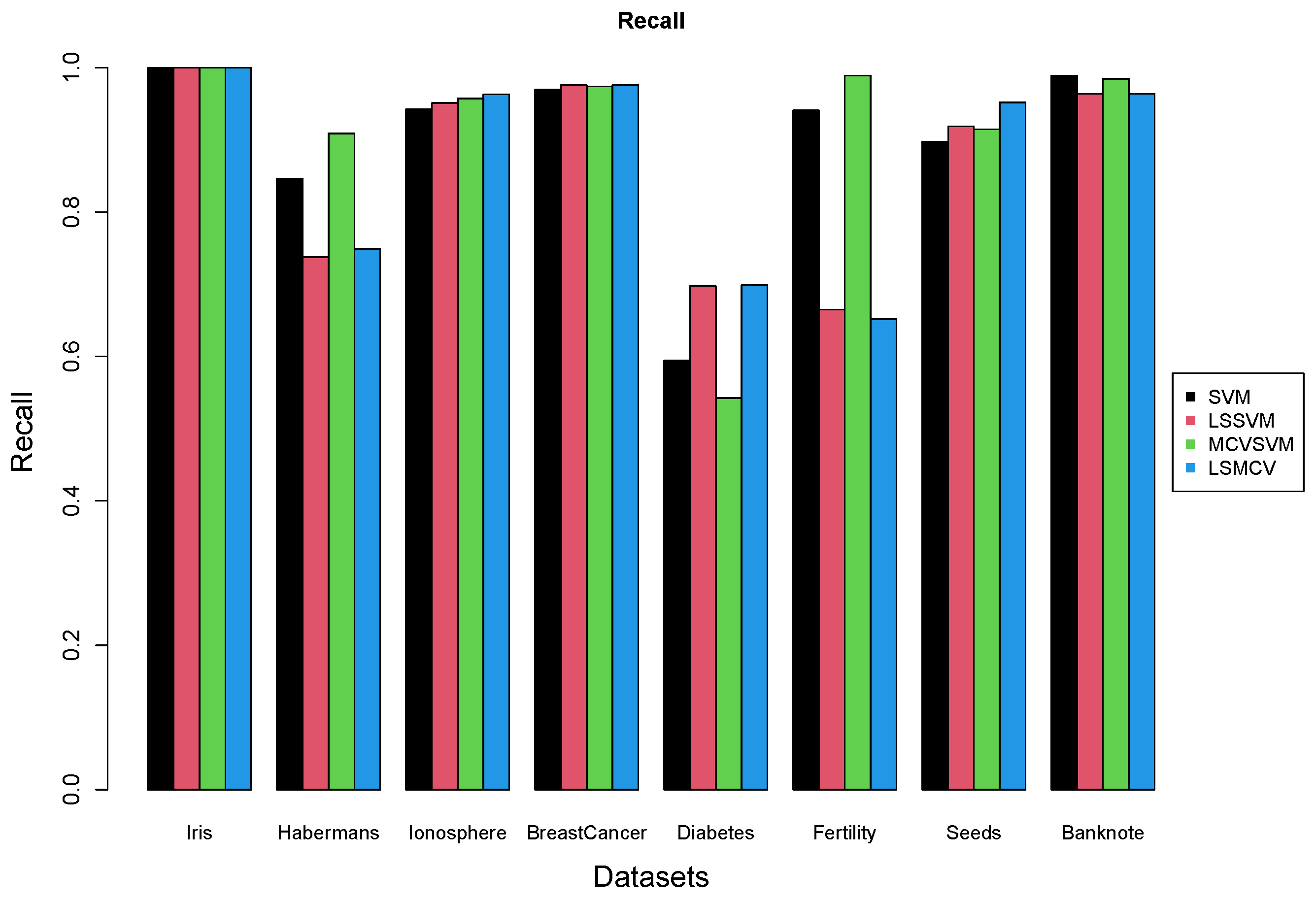
5. Real Data Experiments

To demonstrate the performance of the new algorithm, we ran an analysis on eight datasets. All eight datasets are from the UCI Machine Learning repository. Since we do not discuss multicategory SVM approaches in this paper, we have chosen datasets that have only two classes, or, in the case of multiple classes, we merged together all the classes but the first to create two classes. The datasets we used are summarized in Table 1.
We split the data into 60% training, 20% testing, and 20% validation datasets and we reported the misclassification rates in the validation dataset, where we use the linear kernel to find an optimal hyperplane and calculate the quantities. The reported quantities in this paper are the average of 10 iterations. Table 2 summarizes the mean misclassification rates and the standard errors. We see that the four algorithms are relatively close, and the least squares approaches (either the classic LSSVM or our proposed methodology, which combines the least squares approach with the minimum class variance) to performed slightly better in most cases.
In addition to the misclassification rate, we calculated the average value of the precision, the recall, and the F1 score in each dataset. We present the results in Figure 1, Figure 2 and Figure 3. As we can see, the performance of the algorithms is very similar across the different metrics. In some cases, our method performs better than the rest (i.e., diabetes and seeds datasets) and in some cases, not as well (i.e., fertility). The differences are small, with our method being very close to the LSSVM performance. In the seeds dataset, our method is better than the LSSVM algorithm, but, in that case, it is very close to the MCVSVM algorithm. This is another indication that our method is able to simultaneously capture the advantages that both the LSSVM and MCVSVM algorithms offer.
Most importantly, we can see in Table 3 that both the least square approaches are significantly faster. This difference is actually statistically significant. To demonstrate this, we ran two sample paired nonparametric tests, i.e., Wilcoxon signed-rank tests, for all six pairs of algorithms. The comparison between our algorithm, LSMCVSVM, and SVM gives a p-value of 0.0078, and the comparison between LSMCVSVM with MCVSVM gives a similar p-value, i.e., 0.0078. The comparison between LSSVM and LSMCVSVM gives a nonsignificant p-value (0.7422), which is expected as both algorithms use the least squares approach and have similar running times. The computational gains can be further signified if one extrapolates this difference in massive datasets where we may have a few million datapoints.
For the interested reader, the codes are available at [19].

6. Conclusions

In this work, we presented a new algorithm for classification which combines two existing algorithms. The first algorithm used is the LSSVM, which is one of the fastest algorithms in the SVM family of algorithms, as it has analytical solution. The second algorithm is the MCVSVM, which is an algorithm that generalizes better than the classic SVM algorithm, and it also allows for the variability in each class to be taken into account. The new algorithm, called LSMCVSVM, as demonstrated in our numerical section, has comparable performance with other classic SVM algorithms, like the SVM, LSSVM, and MCVSVM, but it runs in a fraction of time due to the fact that there is no need to solve a quadratic programming optimization problem as one can find an analytic solution. The computational gains of the new algorithms are similar to the computational gains of the LSSVM and the performance is very similar to the MCVSVM, demonstrating that the combination of the two algorithms creates a new algorithm which also combines the advantages of the two algorithms.
Another important aspect of the new method and an important contribution of this paper is the use of principal projections to address the singularity in the solution of r . Since the solution of LSMCVSVM requires the use of the inverse of a matrix, without this equivalence, we would not have been able to apply this algorithm to large p small n problems. This provides a way to do this, without the need to introduce other difficult and time-consuming methods for inverse matrix approximation to find the singularity in the matrix.

Other Approaches and Future Work

The SVM literature is full of variants of the classic SVM algorithm since its introduction by [1]. One can combine any of the existing algorithms and create new algorithms, which can be extremely valuable tools in the classification framework. For example, one of the many ideas that can be implemented is the combination of our algorithm with the two-cost alternative, which is an idea used to handle imbalanced classes, i.e., problems where one class has a lot more points than the other class. In this case, it makes sense that a misclassification from the small class should be more costly. Therefore, ref. [20] proposed the use of two different costs or penalties. By giving a bigger penalty to the smaller class, we try to minimize the effect of misclassifying one point may have. The theoretical development of this variation is similar to the development demonstrated in the previous section for LSMCVSVM; therefore, we present only a small introductory development and leave further development for future work. We start first by stating the optimization problem people need to optimize, which is the minimization of the following objective function:
min 1 2 ψ T Σ w ψ + λ 1 i : y i = 1 n ξ i 2 + λ 1 i : y i = 1 n ξ i 2
under the equality constraints:
y i ( ψ T x i t ) = 1 ξ i ,
If someone follows the proper procedure, then the solution will be:
r = Λ D Σ w + ( X ) T X 1 X T D Y 1 n
where Λ D is the diagonal matrix that has, as the i th entry on the main diagonal, the quantity ( 1 / λ 1 ) I ( Y i = 1 ) + ( 1 / λ 1 ) I ( Y i = 1 ) , where I ( · ) denotes the indicator function. There are different suggestions to select the two different costs, although the most frequently used in the literature (see for example [21]) is λ 1 / λ 1 = n 1 / n 1 where n i is the number of observations in class i = { 1 , 1 } . Here, we emphasize that the topic of imbalance is a very rich topic, in terms of literature, with hundred methods available on how to address imbalance in the SVM framework (see [22] for a comprehensive overview). Therefore, we prefer to address this topic separately, as this will give us a way to check the impact that our new algorithm may have in addressing imbalance.
In addition to the development of new classification methodologies by utilizing the SVM algorithm and its variants, in the literature, there are more ideas which use the SVM type of algorithms to implement new approaches. One such way of utilizing the new algorithm beyond the classification framework is its use in the sufficient dimension reduction (SDR) framework. Recently, SVMs have been introduced extensively in SDR (see for example [23,24,25]), and, therefore, much more developments may be studied in SDR by utilizing new algorithms. The least squares approach, which allows for the use of analytic solution to estimate the optimal hyperplane, might lead to the use of a real-time dimension reduction method, as was demonstrated by [23].
Finally, an anonymous reviewer pointed out to us that there was a similar work that was performed much earlier than our work. The work by [26] discusses a similar idea, as indicated by the title. Unfortunately, we were not able to find a version of that paper to read and compare it to our work. The only pointer to the paper we found online was in Chinese, which was impossible for us to read. It may be an interesting exercise for someone to compare our developments with their development and see if there are any differences.

Author Contributions

Conceptualization: A.A.; Methodology: M.P. and A.A.; Software: M.P.; Formal Analysis: M.P.; Resources: M.P. and A.A.; writing—original draft; Michalis Panagides; writing—review and editing; A.A.; visualization; A.A.; supervision: A.A. All authors have read and agreed to the published version of the manuscript.

Funding

This research received no external funding.

Data Availability Statement

All the datasets are publicly available and sources are presented in Table 1.

Acknowledgments

The authors would like to thank an Associate Editor and three anonymous reviewers for their input which have improved the content and presentation of our idea in this manuscript.

Conflicts of Interest

The authors declare no conflicts of interest.

References

  1. Cortes, C.; Vapnik, V. Support-vector networks. Mach. Learn. 1995, 20, 273–297. [Google Scholar] [CrossRef]
  2. Liu, W.; Ci, L.; Liu, L. A New Method of Fuzzy Support Vector Machine Algorithm for Intrusion Detection. Appl. Sci. 2020, 10, 1065. [Google Scholar] [CrossRef]
  3. Razaque, A.; Mohamed, B.H.F.; Muder, A.; Munif, A.; Bandar, A. Improved Support Vector Machine Enabled Radial Basis Function and Linear Variants for Remote Sensing Image Classification. Sensors 2021, 21, 4431. [Google Scholar] [CrossRef] [PubMed]
  4. Panup, W.; Wachirapong, R.; Rabian, W. A Novel Twin Support Vector Machine with Generalized Pinball Loss Function for Pattern Classification. Symmetry 2022, 14, 289. [Google Scholar] [CrossRef]
  5. Han, K.-X.; Chien, W.; Chiu, C.-C.; Cheng, Y.-T. Application of Support Vector Machine (SVM) in the Sentiment Analysis of Twitter DataSet. Appl. Sci. 2020, 10, 1125. [Google Scholar] [CrossRef]
  6. Sheykhmousa, M.; Mahdianpari, M.; Ghanbari, H.; Mohammadimanesh, F.; Ghamisi, P.; Homayouni, S. Support Vector Machine Versus Random Forest for Remote Sensing Image Classification: A Meta-Analysis and Systematic Review. IEEE J. Sel. Top. Appl. Earth Obs. Remote Sens. 2020, 13, 6308–6325. [Google Scholar] [CrossRef]
  7. Ehsan, H.; Lahmer, T.; Kumari, V.; Jadhav, K. Application of Support Vector Machine Modeling for the Rapid Seismic Hazard Safety Evaluation of Existing Buildings. Energies 2020, 13, 3340. [Google Scholar] [CrossRef]
  8. Suykens, J.A.K.; Vandewalle, J. Least Squares Support Vector Machine classifiers. Neural Process. Lett. 1999, 9, 293–300. [Google Scholar] [CrossRef]
  9. Zafeiriou, S.; Tefas, A.; Pitas, I. Minimum Class Variance Support Vector Machines. IEEE Trans. Image Process. 2006, 16, 2551–2564. [Google Scholar] [CrossRef] [PubMed]
  10. Fisher, R.A. The Use of Multiple Measurements in Taxonomic Problems. Ann. Eugen. 1936, 7, 179–188. [Google Scholar] [CrossRef]
  11. Fisher, R.A. Iris. UCI Machine Learning Repository. 1988. Available online: https://archive.ics.uci.edu/dataset/53/iris (accessed on 23 January 2024). [CrossRef]
  12. Haberman, S. Haberman’s Survival. UCI Machine Learning Repository. 1999. Available online: https://archive.ics.uci.edu/dataset/43/haberman+s+survival (accessed on 23 January 2024). [CrossRef]
  13. Sigillito, V.; Wing, S.; Hutton, L.; Baker, K. Ionosphere. UCI Machine Learning Repository. 1989. Available online: https://archive.ics.uci.edu/dataset/52/ionosphere (accessed on 23 January 2024). [CrossRef]
  14. Wolberg, W. Breast Cancer Wisconsin (Original). UCI Machine Learning Repository. 1992. Available online: https://archive.ics.uci.edu/dataset/15/breast+cancer+wisconsin+original (accessed on 23 January 2024). [CrossRef]
  15. Kahn, M. Diabetes. UCI Machine Learning Repository. Available online: https://archive.ics.uci.edu/dataset/34/diabetes (accessed on 23 January 2024). [CrossRef]
  16. Gil, D.; Girela, J. Fertility. UCI Machine Learning Repository. 2013. Available online: https://archive.ics.uci.edu/dataset/244/fertility (accessed on 23 January 2024). [CrossRef]
  17. Charytanowicz, M.; Niewczas, J.; Kulczycki, P.; Kowalski, P.; Lukasik, S. Seeds. UCI Machine Learning Repository. 2012. Available online: https://archive.ics.uci.edu/dataset/236/seeds (accessed on 23 January 2024). [CrossRef]
  18. Lohweg, V. Banknote Authentication. UCI Machine Learning Repository. 2013. Available online: https://archive.ics.uci.edu/dataset/267/banknote+authentication (accessed on 23 January 2024). [CrossRef]
  19. Panayides, M.; Artemiou, A. LSMCV-SVM Comparisons with Other SVMs. Zenodo. 2024. Available online: https://zenodo.org/records/10476188 (accessed on 23 January 2024). [CrossRef]
  20. Veropoulos, K.; Campbell, C.; Cristianini, N. Controlling the sensitivity of support vector vector machines. In Proceedings of the Sixteenth International Joint Conference on Artificial Intelligence (IJCAI ’99), Workshop ML3, Stockholm, Sweden, 31 July–6 August 1999; pp. 55–60. [Google Scholar]
  21. Artemiou, A.; Shu, M. A cost based reweighed scheme of Principal Support Vector Machine. Top. Nonparamet. Stat. Springer Proc. Math. Stat. 2014, 74, 1–22. [Google Scholar]
  22. He, H.; Garcia, E.A. Learning from Imbalanced Data. IEEE Trans. Knowl. Data Eng. 2009, 21, 1263–1284. [Google Scholar] [CrossRef]
  23. Artemiou, A.; Dong, Y.; Shin, S.J. Real-time sufficient dimension reduction through principal least squares support vector machines. Pattern Recognit. 2021, 112, 107768. [Google Scholar] [CrossRef]
  24. Jang, H.J.; Shin, S.J.; Artemiou, A. Principal weighted least square support vector machine: An online dimension-reduction tool for binary classification. Comput. Stat. Data Anal. 2023, 187, 107818. [Google Scholar] [CrossRef]
  25. Li, B.; Artemiou, A.; Li, L. Principal Support Vector Machines for linear and nonlinear sufficient dimension reduction. Ann. Stat. 2011, 39, 3182–3210. [Google Scholar] [CrossRef]
  26. Wang, X.-M.; Wang, S.-T. Least-Square-based Minimum Class Variance Support Vector Machines. Jisuanji Gongcheng Comput. Eng. 2010, 36, 12. [Google Scholar]
Figure 1. Barcharts show the precision for the four different algorithms on the 8 datasets.
Computers 13 00034 g001
Figure 2. Barcharts show the recall for the four different algorithms on the 8 datasets.
Computers 13 00034 g002
Figure 3. Barcharts show the F1 score for the four different algorithms on the 8 datasets.
Computers 13 00034 g003
Table 1. Dataset description. All source links start with ‘https://archive.ics.uci.edu/dataset’ and were valid on the final access on 25 January 2024.
DatasetObservationsFeaturesSource, Citation
Iris1504 /53/iris, [11]
Haberman’s3063 /43/haberman+s+survival, [12]
Ionosphere35134 /52/ionosphere, [13]
Breast Cancer6999 /15/breast+cancer+wisconsin+original, [14]
Diabetes≈253,00021 /891/cdc+diabetes+health+indicators, [15]
Fertility10010 /244/fertility, [16]
Seeds2107 /dataset/236/seeds, [17]
Banknote13725 /267/banknote+authentication, [18]
Table 2. Overall misclassification errors (standard errors) for each algorithm in each dataset. The best algorithm for each dataset is highlighted in bold.
AlgorithmSVMLS SVMMCV SVMLSMCV SVM
Datasets
Iris0 (0)0 (0)0 (0)0 (0)
Haberman’s0.27 (0.002)0.25 (0.002)0.27 (0.002)0.25 (0.002)
Ionosphere0.14 (0.002)0.14 (0.002)0.14 (0.002)0.14 (0.002)
Breast Cancer0.04 (0.000)0.04 (0.000)0.04 (0.000)0.04 (0.000)
Diabetes0.24 (0.001)0.23 (0.001)0.24 (0.001)0.23 (0.001)
Fertility0.17 (0.010)0.12 (0.005)0.17 (0.009)0.12 (0.005)
Seeds0.07 (0.001)0.06 (0.001)0.04 (0.001)0.03 (0.001)
Banknote0.01 (0.000)0.03 (0.000)0.01 (0.000)0.03 (0.000)
Table 3. Duration of each algorithm for each dataset (in seconds)—the faster algorithm for each dataset is highlighted in bold.
AlgorithmSVMLS SVMMCV SVMLSMCV
Datasets
Iris0.2290.009310.2050.0207
Haberman’s0.9530.03050.7830.0334
Ionosphere1.290.05931.120.0784
Breast Cancer8.790.2416.340.217
Diabetes10.40.3428.0030.307
Fertility0.1390.007860.1250.016
Seeds0.4410.01640.3720.0224
Banknote59.31.6749.11.42
Disclaimer/Publisher’s Note: The statements, opinions and data contained in all publications are solely those of the individual author(s) and contributor(s) and not of MDPI and/or the editor(s). MDPI and/or the editor(s) disclaim responsibility for any injury to people or property resulting from any ideas, methods, instructions or products referred to in the content.

