Employing Different Algorithms of Lightweight Convolutional Neural Network Models in Image Distortion Classification

Abstract

The majority of applications use automatic image recognition technologies to carry out a range of tasks. Therefore, it is crucial to identify and classify image distortions to improve image quality. Despite efforts in this area, there are still many challenges in accurately and reliably classifying distorted images. In this paper, we offer a comprehensive analysis of models of both non-lightweight and lightweight deep convolutional neural networks (CNNs) for the classification of distorted images. Subsequently, an effective method is proposed to enhance the overall performance of distortion image classification. This method involves selecting features from the pretrained models’ capabilities and using a strong classifier. The experiments utilized the kadid10k dataset to assess the effectiveness of the results. The K-nearest neighbor (KNN) classifier showed better performance than the naïve classifier in terms of accuracy, precision, error rate, recall and F1 score. Additionally, SqueezeNet outperformed other deep CNN models, both lightweight and non-lightweight, across every evaluation metric. The experimental results demonstrate that combining SqueezeNet with KNN can effectively and accurately classify distorted images into the correct categories. The proposed SqueezeNet-KNN method achieved an accuracy rate of 89%. As detailed in the results section, the proposed method outperforms state-of-the-art methods in accuracy, precision, error, recall, and F1 score measures.

1. Introduction

The advancement of information technology and the advent of the Internet of Things (IOT) have led to a rise in the need for image processing and a growing quantity of hardware with cameras for use in everyday activities, company operations, and industry. Numerous apps and programs exchange and use a huge number of images every day. There are many ways in which these images can be distorted. For instance, (1) poor light causing noise, (2) the movement of the camera, and (3) surveillance images taken through inclement weather or a low-quality devices [1]. The well-known kinds of distortion include ‘Blur’, ‘Noise’, ‘Sharpness’, ‘Contrast Change’, and ‘Compression’ [2], as shown in Figure 1.

Figure 1. Common Distortion Types. (a) Original Image; (b) Blur; (c) Noise; (d) Sharpness; (e) Contrast Change; (f) Compression.

Generally, image classification employs a classifier to determine the group of objects after manually obtaining features or using feature learning techniques to define the entire image. Therefore, knowing how to extract the image’s features is crucial [3]. As shown by the taxonomy in Figure 2, distorted image classification methods may generally be divided into three categories: traditional, deep, and hybrid.

Figure 2. The Taxonomy of Distortion Image Classification Techniques.

The performance of most image detection/classification methods is impacted by these types of distortion. This has motivated researchers to develop systems that can automatically detect and classify distortions by type, making it easier to address and improve these distortions. This will ultimately increase the performance of these approaches.

To address challenging feature engineering problems and the often time-consuming need for domain knowledge, deep learning techniques have been applied to image detection/classification. Deep learning algorithms offer accurate understandings and predictions by identifying complex patterns in text, audio, image, and other types of data. Convolutional neural networks (CNNs) are a popular deep learning technique that works effectively well for image classification tasks [4].

Most conventional image classification techniques based on CNN follow an end-to-end learning procedure. In this approach, the network handles training and prediction using only the original image as input, producing the final output directly from this input.

However, CNNs remain susceptible to distorted images. Even a small amount of noise or blur can significantly affect their performance in various computer vision tasks such as object detection, image registration and segmentation. Most research in the literature addresses this issue by fine-tuning pretrained CNNs using a combined or mutually distinct set of distorted training data [5]. Since lightweight CNN models provide real-time processing with minimum computational resources and strike a balance between effectiveness and precision, they are crucial for classifying image distortion.

Previous methods rely on some features from a pretrained model. These methods often suffer from the following issues: (1) difficulty in discovering and extracting more significant and effective features; (2) limiting training data; (3) poor classification accuracy due to the use of laborious and imprecise features for image identification; (4) a large feature vector dimension that leads to substantial computational load.

Creating an efficient image detection model that addresses the previously listed problems is the most challenging task. Therefore, the goal of this research is to analyze and evaluate the role of lightweight and non-lightweight deep CNN models in classifying different types of image distortions and determining which model is more effective. Subsequently, the proposed method was introduced, which relies on selected features from pretrained models and classifiers. The primary objectives of the proposed method are to increase the accuracy of classifying distorted images, reduce the likelihood of incorrect classifications, and collect relevant data.

Numerous efforts have been made to address the primary research issue and improve detection accuracy, and can be summarized as follows:

• An analysis is conducted on how image distortion affects both lightweight and non-lightweight deep CNN models.
• Experimental findings indicate that the proposed approach exhibits resilience against different kinds of image distortion. The performance under 25 types of distortion across five levels of severity are examined.
• Several important features are extracted from the last fully connected layers of lightweight and non-lightweight deep CNN models such as SqueezeNet, DenseNet201, and MobileNetv2 models.
• The training process is simplified by leveraging models such as MobileNet-v2, SqueezeNet, and DenseNet201, which are initially trained as feature extractors, followed by using PCA to produce smaller feature sets.
• Utilizing the KADID-10k dataset, the proposed distortion image classification method combining SqueezeNet and KNN achieved the best performance across all evaluation metrics.
• The proposed distortion image classification technique is based on a lightweight structure that needs minimal time and effort.

The remaining components of the paper are organized as follows: A review of the related works is discussed in Section 2. Section 3 describes the characteristics of the pretrained CNN models. Section 4 provides a description of the proposed approach. Section 5 presents the experimental results, their interpretation and their significance. The paper concludes in Section 6.

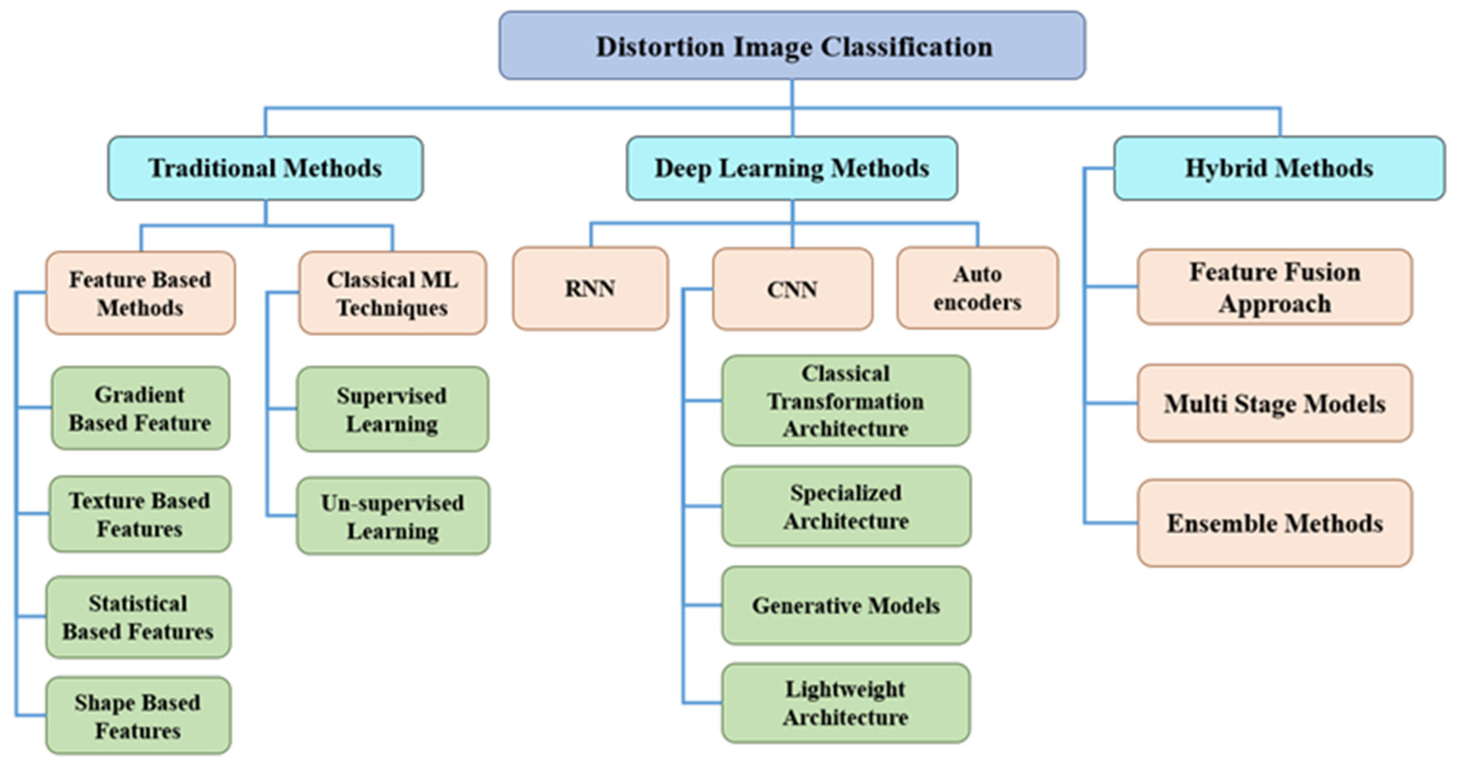
2. Related Works

The majority of applications regard distortion classification to be a difficult issue. There are not many works that expressly cover it. Numerous classification approaches have been presented in the literature for each of these techniques; all of them are based on both hand-crafted and generic features. Using hand-crafted features includes the drawback of being non-generic and specific to the application.

However, convolutional neural networks (CNNs) enable the solution of this problem by creating an automated feature learning technique that is applicable to a wide range of distortions. Moreover, they have the capacity to pick up additional informative and discriminative features. Therefore, deep features are now a serious contender to replace hand-crafted ones.

This method does not rely on the manual extraction of certain image features. Consequently, this is CNNs’ primary advantage for image classification. There are not many methods in the literature that address the impact of image distortion issues, despite the fact that deep networks are susceptible to distortion or quality degradation [5,6].

Zhou et al. [7] proposed a distortion detection method based on a DNN classifier across various distortions. It demonstrated the fine-tuning and retraining methods for minimizing the impact of image distortions. However, with different kinds of distortions, a single fine-tuning network might not function adequately. Yu Li and Lizhuang Liu [8] proposed a distortion detection method based on a pre-trained convolutional neural network (CNN). In the classification stage, the support vector machine (SVM) model is applied. The proposed approach can correctly detect distorted images, according to the results of experiments conducted on real images. Dodge and Karam [9] presented an image identification based on deep network. The experimental findings demonstrate that visual distortions can have a substantial impact on the accuracy of deep networks. The VGG-16 design has been demonstrated to be more resilient than the other networks. He et al. [10] proposed a distortion detection method based on different deep convolutional neural networks (CNNs). In the classification stage, the SoftMax model is applied. It is clear, therefore, that the SoftMax model performs poorly in classifying the distortions. Zhou et al. [7] proposed the systematic investigation of the impact of image distortions on the deep neural network (DNN) image classifiers. In the classification stage, the DNN model is applied. Basu et al. [11] proposed a distortion detection method based on DNN, which relies on modified deep belief nets. They presented positive findings on the noisy n-MNIST dataset. Minho et al. [12] proposed a method based on a selective deep convolutional neural network (DCNN) to detect various kinds and intensities of distortions. The results of the studies with increased kinds and intensities of image distortion demonstrate the strong scalability of selective DCNN. Saurabh et al. [13] proposed automatic detection and classification of blurred images based on convolution neural networks (CNNs). A dataset of 20,000 digital photos sourced from various sources and tagged with two different categories was used to train the proposed CNN model. Rui Wang et al. [14] proposed an ensemble CNN that included the Simplified Alex net with the Simple Google net to classify four types of blurry photos. When compared to Alex net and Google net independently, the experimental findings demonstrated that the ensemble classifier completed the classification task significantly faster. Wang et al. [15] proposed using ensemble support vector machine structures to classify three types of blurry photos. The BHBID Database was used to conduct the experiment. In the classification stage, the SVM classifier model was applied. Hossain et al. [16] proposed a distortion detection method based on DCT and CNN (DCT-Net). A deep network module based on the discrete cosine transform was constructed on top of VGG16. The experimental results demonstrate that DCT-Net performs better than other, similar networks in previous research and, once trained, generalizes effectively to a wide range of undetected distortions.

The majority of earlier techniques have the following problems. The impact of the distorted dataset size: Overfitting could occur by training the model on a small distorted dataset when the model is extremely deep; the majority of datasets, in general, only include homogenous distortion patterns, which facilitate easy prediction. The reality that images might have a variety of different kinds of distortion makes distortion detection challenging. Extraction of robust and efficient features, heavy weight, poor classification percentage due to the use of laborious and imprecise features to identify images, and a large feature vector dimension lead to a substantial computational load. Therefore, by improving the accuracy of identifying distorted images, decreasing the possibility of inaccurate classifications, and gathering appropriate information, the proposed approach aims to address the majority of the aforementioned limitations.

3. Preliminaries: Classic CNN Models

Because the training procedure is time-consuming, pretrained CNN models have been employed as feature extractors to reduce the costs associated with training. Various pretrained CNN models have been developed, and these already-trained models have been used for several different multi-class classification problems [17]. Lightweight deep learning (DL) refers to the processes of condensing deep CNN models into smaller versions that can run on edge devices despite their constrained computing power and availability of resources while preserving the same performance as the original model [18]. In the subsections that follow, we will give a brief overview of the pretrained models used in this research. The key features across multiple pretrained networks are listed in Table 1.

Table 1. The most common pretrained CNN model properties.

Model	Mobile Net v2	DenseNet201	SqueezeNet
Year	2018	2016	2016
Image Dimensions	224 × 224 × 3	224 × 224 × 3	227 × 227
Number of Layers	53	201	18
Number of Parameters	3.5 million	20 million	1.24 million
Feature Dimension	1344	1000	1000
Design	lightweight	non-lightweight	lightweight

3.1. Lightweight Deep CNN Models

Most applications employ complex and deep networks to enhance accuracy, but they overlook two critical factors: speed and size. In this section, we will provide more compact and effective models designed to perform the recognition tasks quickly on platforms with limited processing power.

3.1.1. SqueezeNet

Lower parameter computationally neural networks and a miniaturized network model structure called SqueezeNet were suggested by F. N. Iandola et al. in 2016 [19]. SqueezeNet consists of 15 layers, which are split into five different levels: two layers for convolution, three layers for pooling, eight layers for fire, one global average layer for pooling, and one output layer for SoftMax. SqueezeNet benefits are demonstrated by comparison with the AlexNet model. SqueezeNet compresses the model volume to roughly 1/510th its original size while guaranteeing that the precision is maintained despite a roughly 50-fold reduction in parameters [20].

3.1.2. MobileNetv2

There are 53 layers in the lightweight MobileNetV2 convolutional neural network (CNN). The architecture of MobileNetV2 [21] starts with a sequence of convolutional layers and continues with depth-wise differentiated convolutions, inverted residuals, bottleneck design, linear bottlenecks, and squeeze-and-excitation (SE) blocks. Together, these elements enable the model to retain its capacity to capture intricate features while requiring fewer calculations and parameters. There are various benefits of classifying images using MobileNetV2. First of all, the architecture is lightweight. Second, when compared with bigger and more computationally costly models, MobileNetV2 obtains comparative accuracy. Finally, the model is appropriate for applications that operate in real time thanks to its compact size, which allows for speedier inference times.

3.2. Non-Lightweight Deep CNN Models

Overall, DenseNet-201 [22] has 201 layers. Conventional convolution connects each layer to the following layer. Each of the layers in DenseNet has a feed-forward connection to each subsequent layer. Implicit deep supervision results from giving each layer immediate accessibility to the gradients derived from the initial input signal and the corresponding loss function.

4. Our Proposed Method

The approach for the comparative study and the recommended method for distorted image classification involves four primary processes comprising data preparation, feature extraction, feature selection, classification, and evaluation. A procedural graph illustrating the method and its comparison steps is shown in Figure 3. Detailed information for each step is provided in the following subsections.

Figure 3. Comparative Study and the Proposed Methodology.

• STEP 1: Data Preparation

In this step, the technique modifies the size of the distorted images, which are adjusted to match the input size of each pretrained CNN model. For the DenseNet201 and MobileNetv2 models, images are resized to (224, 224) pixels, and for the SqueezeNet model, the images are resized to (227, 227) pixels. The resizing is required to ensure that the input dimensions are compatible with the respective models for accurate feature extraction and subsequent processing.

• STEP 2: Feature Extraction

Pretrained models are used as feature extractors for distorted image detection because they have already learned how to extract relevant features from large datasets. In order to train these deep learning models on smaller datasets without encountering the issue of overfitting, transfer learning is used. Transfer learning allows these models to leverage the knowledge gained from vast amounts of data and apply it to new tasks with limited data.

• STEP 2.1: DenseNet201 Feature Extraction

Algorithm 1 depicts a general framework for DenseNet201 feature extraction. The final fully connected layers (fc1000) yield a 1 × 1000 feature vector, which is the DenseNet201 feature vector.

Algorithm 1 DenseNet201 model as feature extraction

Input: Distorted Image from dataset. Output: 1 × 1000 features vector dimension. Begin For 1: Import the dataset images and perform the following preprocessing steps in accordance with DenseNet201 requirements:   1.1: Every image entry should be limited to a value between 0 and 255.   1.2: For every image, adjust the resolution to (224 × 224). 2: Import Pre-trained DenseNet201 Model: 3: Import DenseNet201 model weights. 4: Eliminate the layer of classification. The final fully connected (FC) layers of the model are either absent or have been removed. 5: Select the Feature Extraction Layer: Create a brand-new model only for the feature extraction, then carry out the subsequent loop steps:   5.1: Go over every image in the dataset one by one.   5.2: Send the image up to the selected feature extraction layer via the Pre-trained DenseNet201 Model.   5.3: Extract features from the selected layer (“fc1000”).   5.4: Save the features that were extracted into an array. 6: Apply the flattened method to reduce the dimensions of the features array into one. 7: Print the flattened array. 8: Save the 1000 feature vector that was produced. End for End

• STEP 2.2: SqueezeNet Features Extraction

Algorithm 2 provides a general framework for SqueezeNet feature extraction. The final fully connected layers (avg_pool10) yield a 1 × 1000 feature vector, which is the SqueezeNet feature vector.

Algorithm 2 SqueezeNet model as feature extraction

Input: Distorted Image from dataset. Output: 1 × 1000 features vector dimension. Begin For 1: Import the dataset images and perform the following preprocessing steps in accordance with SqueezeNet requirements:   1.1: Every image entry should be limited to a value between 0 and 255.   1.2: For every image, adjust the resolution to (227 × 227). 2: Import Pre-trained SqueezeNet Model: 3: Import SqueezeNet model weights. 4: Eliminate the layer of classification. The final fully connected (FC) layers of the model are either absent or have been removed. 5: Select the Feature Extraction Layer: Create a brand-new model only for the feature extraction, then carry out the subsequent loop steps:   5.1: Go over every image in the dataset one by one.   5.2: Send the image up to the selected feature extraction layer via the Pre-trained SqueezeNet Model.   5.3: Extract features from the selected layer (“avg_pool10”).   5.4: Save the features that were extracted into an array. 6: Apply the flattened method to reduce the dimensions of the features array into one. 7: Print the flattened array. 8: Save the 1000 feature vector that was produced. End for End

• STEP 2.3: MobileNetv2 Feature Extraction

Algorithm 3 provides a general framework for MobileNetV2 feature extraction. The final fully connected layers (block_12_add) yield a 1 × 1344 feature vector, which is the MobileNetV2 feature vector.

Algorithm 3 MobileNetV2 model as feature extraction

Input: Distorted Image from dataset. Output: 1 × 1344 features vector dimension. Begin For 1: Import the dataset images and perform the following preprocessing steps in accordance with MobileNetV2 requirements:   1.1: Every image entry should be limited to a value between 0 and 255.   1.2: For every image, adjust the resolution to (224 × 224). 2: Import Pre-trained MobileNetV2 Model: 3: Import MobileNetV2 model weights. 4: Eliminate the layer of classification. The final fully connected (FC) layers of the model are either absent or have been removed. 5: Select the Feature Extraction Layer: Create a brand-new model only for the feature extraction, then carry out the subsequent loop steps:   5.1: Go over every image in the dataset one by one.   5.2: Send the image up to the selected feature extraction layer via the Pre-trained MobileNetV2 Model.   5.3: Extract features from the selected layer (“block_12_add”).   5.4: Save the features that were extracted into an array. 6: Apply the flattened method to reduce the dimensions of the features array into one. 7: Print the flattened array. 8: Save the 1344 feature vector that was produced. End for End

• STEP 3: Apply Feature Selection Method

A popular method for dimensionality reduction in feature selection is Principal Component Analysis (PCA) [23]. The input data was used to extract the features of the pretrained models; the most effective features were subsequently selected and utilized in the classification step. The following (Algorithm 4) is a description of an algorithm for applying PCA to feature selection:

Algorithm 4 PCA Feature selection

Input: Feature Extracted Vector. Output: Selected Feature Vector. Begin For 1: Import the Feature extracted vector. 2: To guarantee that every feature has an equal scale, standardize or normalize the feature extraction vector using the following sub steps:   2.1: Calculate the mean of each feature and divide it by the standard deviation.   2.2: As required by PCA, this guarantees that every feature has a mean of 0 and a standard deviation of 1. 3: Determine the standardized features’ covariance matrix. The correlations between various features are revealed by the covariance matrix. 4: Determine the eigenvalues and eigenvectors covariance matrixes. To determine the eigenvalues and eigenvectors of the covariance matrix, apply eigen decomposition. 5: Choose Principal Components: Choose the top k eigenvectors that match the biggest eigenvalues by sorting the eigenvalues in descending order. These outputs are the Principal components. 6: Project Data onto Principal Components: To generate the reduced dimensional feature space, project the standardized data onto the principal components that have been chosen. End for End

• STEP 4: Classification

To evaluate the effectiveness of the model and the selected features, it is necessary to perform a classification step. The selected features are used to train a different classifier, which then classifies the different types of distortion. There are numerous photos, and the majority of them have various types of distortion. Therefore, an algorithm that can detect these particular types of distortion and classify the image as distorted needs to be discovered. This type of prediction classification challenge can be resolved easily using KNN and the naive Bayes method. For this reason, we used K-nearest neighbor (KNN) and naive Bayes (NB) as effective classifiers in the present research for classifying the distorted images.

• STEP 4.1: K-Nearest Neighbor (KNN) Classifier.

The K-nearest neighbor (KNN) classifier [24] is a non-parametric, easy to understand, and effective machine learning algorithm used for classification and regression tasks. It entails classifying a sample based on the k training set samples that are most similar to it. KNN has several advantages: it is easy to use, does not require a detailed training step, and works well in a variety of applications, especially when working with big sets of training data [25]. In order to reduce overfitting and enhance generalization, the optimum K is chosen.

Here is the procedure to develop a KNN model.

• Training Phase:
  • Training and testing data sets are divided according to the preceding selected feature vectors.
  • KNN is an instance-based learning algorithm; that is, it memorizes the training cases instead of learning a model explicitly.
  • All of the training data points and the labels that go with them are stored.
• Prediction Phase:
  • Determine the distance using a distance metric (such as the Euclidean distance) between each training instance and the test instance.
  • Determine which K training instances are nearest to the test instance in order to find neighbors. In this work, a KNN with a 9-neighbor arrangement was used since overfitting reduces as K increases.
  • Popular Vote (for Classification): Choose the class label that the K nearest neighbors share the greatest amount of.
  • Average (for Regression): Determine the expected value by averaging the values of the K nearest neighbors.

Next, using the training data set, the model is trained. Then, the trained KNN model is evaluated to determine which distortion class it belongs to.

• STEP 4.2: Naïve Bayes (NB) Classifier

The naïve Bayes algorithm is a method of supervised learning that solves classification issues. This depends on the Bayes hypothesis. Furthermore, instead of returning the test point’s label, the naive Bayes probabilistic classifier returns the likelihood that the test point belongs to a class. According to the test data, the naive Bayes classifier’s system learning incorporates the best-rated sample in the relevant class [26]. The naive Bayes algorithm can detect these particular types of distortion and classify the image as distorted, as shown in Figure 4. The naïve Bayes classifier is a highly efficient classification technique that can handle highly dimensional information and facilitates the rapid construction of machine learning models capable of making accurate predictions. Next, using the training data set, the model is trained. Then, the trained NB model is evaluated to determine which distortion class it belongs to.

Figure 4. Mechanism of Naïve Bayes Classifier.

• STEP 4.3: The Logistic Regression Classifier.

The logistic regression is known as statistical regression model, and it is based on ordinary regression [23]. The goal of logistic regression is to identify the most effective model for analyzing the correlation between a set of uncorrelated variables (predictor) and a feature of interest that is of a dichotomous nature (outcome variable).

5. Experimental Results and Analysis

The four components of the results that will be covered in this section are available datasets, performance measurement measures, analysis conclusions, and comparisons with various approaches. A few of the requirements, as indicated in Figure 5, were used to carry out the experiment.

Figure 5. Experimentation Properties Description.

5.1. Datasets

The KADID-10k dataset [27] has been used to assess the performance of the recommended approach. A total of 10,125 distorted images make up the entire imbalanced KADID-10k dataset. It is composed of 18 clear images, each of which has undergone five levels of degradation from 25 distortions. Each of the samples in the dataset, as Table 2 demonstrates, falls into one of the 25 categories of distortion. Figure 6 shows the several groups of distorted images in the KADID-10k dataset.

Table 2. Summary of the Kadid-10k Dataset Categories.

Class_ID	Family	Details
		Distortion_Category	Sample_No.
#01, #02, #03	Gaussian blur, Lens blur, Motion blur	Blurs	1215
#04, #05, #06, #07, #08	Color diffusion, Color shift, Color quantization, Color saturation 1, Color saturation 2	Color Distortions	2025
#09, #10,	JPEG2000, JPEG	Compression	810
#11, #12, #13, #14, #15	White noise, White noise in color component, Impulse noise, Multiplicative noise, Denoise	Noise	2025
#16, #17, #18	Brighten, Darken, Mean shift	Brightness Change	1215
#19, #20, #21, #22, #23	Jitter, Non-eccentricity patch, Pixelate, Quantization, Color block	Spatial Distortions	2025
# 24, # 25	High sharpness, Contrast change	Sharpness And Contrast	810
Total		-	10,125

Figure 6. Various Pristine Images. Samples Collected from the KADID-10k Dataset.

Figure 6 indicates the overall amount as well as the spread of samples across the various types of distorted images included in the dataset. It is imperative to emphasize that there is a significant imbalance in the KADID-10k dataset. From Figure 7, we can see that 10% of the images are in the Distortion_Category (Compression, Sharpness, and Contrast), while over 60% of the images are in the Distortion_Category (Color Distortions, Noise, and Spatial Distortions).

Figure 7. The Dispersion of Distortion across Classes inside the KADID-10k Dataset.

5.2. Performance Evaluation Measures

The proposed approach was evaluated using a confusion matrix that included five measures, including accuracy, precision, error, recall, and F-measure. Table 3 contains the mathematical equations and descriptions of these measurements. Each term that can be determined using the aforementioned formulas is described in Figure 8.

Table 3. The Full Description of Each Terms.

Metric	Description	Formula	Eq No
Accuracy	It represents the proportion of accurately recognized images to all images entered.	$\mathrm{A}\mathrm{c}\mathrm{c}\mathrm{u}\mathrm{r}\mathrm{a}\mathrm{c}\mathrm{y}={\displaystyle \frac{TP+TN}{TP+TN+FP+FN}}$	Equation (1)
Precision	The percent of all given images that the classification algorithm properly identified is represented by this number.	$\mathrm{P}\mathrm{r}\mathrm{e}\mathrm{c}\mathrm{i}\mathrm{s}\mathrm{i}\mathrm{o}\mathrm{n}={\displaystyle \frac{TP}{TP+FP}}$	Equation (2)
Error	This is the proportion of every image to the overall number of images that have been mislabeled.	$\mathrm{E}\mathrm{r}\mathrm{r}\mathrm{o}\mathrm{r}={\displaystyle \frac{FP+FN}{TP+TN+FP+FN}}$	Equation (3)
Recall	It represents the proportion of all images belonging to that category that have been accurately classified.	$\mathrm{R}\mathrm{e}\mathrm{c}\mathrm{a}\mathrm{l}\mathrm{l}={\displaystyle \frac{TP}{TP+FN}}$	Equation (4)

Figure 8. A Detailed Description of Every Term [28].

5.3. Evaluation Results

A 10-fold cross-validation technique is used to ensure the accuracy and dependability of the experimental outcomes [29]. In total, 10 tests are carried out, and the process is ultimately evaluated by summing together the outcomes of each experiment.

As is going to be covered in the subsequent section, the results are capable of being evaluated in relation to the best feature and classifier. The features extracted are obtained from lightweight and non-lightweight pretrained CNN models, including SqueezeNet, MobileNet-v2, and DenseNet201.

We choose different percentages of the feature extracted vector (e.g., 25%, 50%, 100%) employing the PCA approach. The feature selection proportion for every one of the chosen lightweight and non-lightweight pretrained CNN models can be seen in Table 4.

Table 4. The Full Summary of Feature Selection Percentage (%) For Every Chosen Pretrained CNN Model.

No	Model	Full Features	Feature Selection Percentage
			100%	50%	25%
1	SqueezeNet	1000	1000	500	250
2	Desnet201	1000	1000	500	250
3	MobileNet-v2	1344	1344	672	236
4	AlexNet	4096	4096	2048	1024

Table 5, Table 6 and Table 7 provide an overview of the performance metrics for SqueezeNet, DenseNet201, and MobileNet-v2 across 25%, 50%, and 100% of the feature extracted vector, respectively, for each distortion class, as well as the overall average of evaluation metrics that was determined after applying each classifier.

Table 5. Evaluation Measures Results of Two Classifiers on SqueezeNet Features Over the Kadid10k Dataset.

Classifier	Class ID	Family Name	Percentage of Selected Features (%)
			SqueezeNet Features-No 100% of Features					SqueezeNet Features-No 50% of Features					SqueezeNet Features-No 25% of Features
			Evaluation Measures (%)					Evaluation Measures (%)					Evaluation Measures (%)
			Accuracy	ER	F1	Precision	Recall	Accuracy	ER	F1	Precision	Recall	Accuracy	ER	F1	Precision	Recall
KNN	#1	Blur	98	02	98	98	100	99	01	99	98	100	99	01	99	99	100
	#2	Brightness Change	86	14	92	96	100	88	12	93	88	100	89	11	92	89	100
	#3	Color Distortion	88	12	94	88	100	89	11	93	87	100	90	10	93	97	100
	#4	Compression	81	19	89	81	100	79	21	88	79	100	82	18	89	80	100
	#5	Noise	91	09	95	91	100	92	08	96	92	100	93	07	95	93	100
	#6	Original	79	21	88	79	100	81	19	89	81	100	83	17	88	82	100
	#7	Sharpness And Contrast	92	08	96	92	100	93	07	96	93	100	93	07	95	91	100
	#8	Spatial Distortion	80	20	89	81	100	81	19	88	78	100	83	17	88	77	100
	Average		86.8	13.1	92.6	88.25	100	87.7	12.25	92.7	87	100	89	11	92.3	88.5	100
Naïve	#1	Blur	89	11	94	100	89	91	09	95	99	91	92	08	95	90	91
	#2	Brightness Change	60	40	73	88	62	81	19	90	87	93	89	11	94	89	100
	#3	Color Distortion	58	42	71	89	59	83	17	92	87	96	85	15	90	87	94
	#4	Compression	52	48	66	74	60	74	26	85	79	92	78	22	88	78	100
	#5	Noise	55	45	69	63	55	91	09	95	91	100	92	08	96	92	100
	#6	Original	63	37	77	78	76	60	40	74	77	72	82	18	90	82	100
	#7	Sharpness And Contrast	54	46	69	93	54	93	07	95	93	95	91	09	95	91	100
	#8	Spatial Distortion	62	38	76	75	78	81	19	89	81	100	88	12	88	86	100
	Average		61.6	38.3	74.3	82.5	66.6	81.7	18.25	89.3	86.7	92.3	87.1	12.8	92	86.8	98.12

Table 6. Evaluation Measures Results of Two Classifiers MobileNet-v2 Features over the Kadid10k Dataset.

Classifier	Class ID	Family Name	Percentage of Selected Features (%)
			SqueezeNet Features-No 100% of Features					SqueezeNet Features-No 50% of Features					SqueezeNet Features-No 25% of Features
			Evaluation Measures (%)					Evaluation Measures (%)					Evaluation Measures (%)
			Accuracy	ER	F1	Precision	Recall	Accuracy	ER	F1	Precision	Recall	Accuracy	ER	F1	Precision	Recall
KNN	#1	Blur	98	02	98	98	100	99	01	99	99	100	99	01	99	99	100
	#2	Brightness Change	86	14	93	88	100	88	12	92	86	100	88	12	94	89	100
	#3	Color Distortion	87	13	93	87	100	88	12	93	88	100	89	11	93	89	100
	#4	Compression	79	21	88	79	100	81	19	89	81	100	82	18	89	80	100
	#5	Noise	91	9	95	91	100	93	07	96	93	100	92	8	95	92	100
	#6	Original	80	20	89	80	100	77	23	87	77	100	79	21	88	79	100
	#7	Sharpness And Contrast	90	10	95	91	100	91	09	95	90	100	93	07	96	93	100
	#8	Spatial Distortion	76	24	88	78	100	77	23	85	77	100	80	20	89	80	100
	Average		85.8	14.1	92.3	86.5	100	86.7	13.25	92	86.3	100	87.7	12.2	92.8	87.6	100
Naïve	#1	Blur	80	20	88	80	100	95	05	97	100	95	98	02	99	100	99
	#2	Brightness Change	51	49	65	88	51	94	06	97	95	99	86	14	92	90	89
	#3	Color Distortion	65	35	78	86	71	72	28	78	93	74	74	26	78	87	80
	#4	Compression	54	46	65	82	54	60	40	62	85	65	64	36	69	82	75
	#5	Noise	48	52	61	95	45	68	32	67	80	70	70	30	75	85	77
	#6	Original	55	45	66	81	56	68	32	69	83	72	69	31	74	81	75
	#7	Sharpness And Contrast	45	54	58	95	41	50	50	56	93	55	53	47	60	60	68
	#8	Spatial Distortion	51	49	62	81	51	60	40	62	83	69	65	35	70	78	72
	Average		56	43	67	86	58	70	29	73	89	74	72	27	77	82	79

Table 7. Evaluation Measures Results of Two Classifiers on DenseNet201 Features over the Kadid10k dataset.

Classifier	Class ID	Family Name	Percentage of Selected Features (%)
			SqueezeNet Features-No 100% of Features					SqueezeNet Features-No 50% of Features					SqueezeNet Features-No 25% of Features
			Evaluation Measures (%)					Evaluation Measures (%)					Evaluation Measures (%)
			Accuracy	ER	F1	Precision	Recall	Accuracy	ER	F1	Precision	Recall	Accuracy	ER	F1	Precision	Recall
KNN	#1	Blur	99	01	99	99	100	98	02	99	98	100	99	01	99	99	100
	#2	Brightness Change	89	11	94	89	100	87	13	93	87	100	89	11	94	89	100
	#3	Color Distortion	87	13	93	82	100	86	14	92	86	100	87	13	93	87	100
	#4	Compression	77	23	88	78	100	79	21	88	79	100	80	20	88	80	100
	#5	Noise	93	07	96	93	100	92	08	96	92	100	91	09	96	93	100
	#6	Original	80	20	89	80	100	78	22	88	78	100	82	18	90	82	100
	#7	Sharpness And Contrast	90	10	95	90	100	91	09	96	93	100	90	10	95	92	100
	#8	Spatial Distortion	78	22	87	78	100	80	20	89	80	100	77	23	79	77	100
	Average		86.6	13.3	92.6	86.12	100	86.3	13.62	92.6	86.6	100	86.8	13.1	91.7	87.3	100
Naïve	#1	Blur	80	20	90	77	89	85	15	88	92	94	90	10	95	97	91
	#2	Brightness Change	56	44	70	90	57	80	20	85	90	97	83	17	92	88	97
	#3	Color Distortion	58	42	71	89	59	81	19	87	88	94	82	18	90	86	92
	#4	Compression	54	46	67	78	58	68	32	78	86	90	85	15	93	90	96
	#5	Noise	55	45	68	92	55	82	18	84	78	99	80	20	88	87	81
	#6	Original	59	41	72	77	68	70	30	79	88	95	90	10	95	91	99
	#7	Sharpness And Contrast	51	49	66	93	51	86	14	90	87	100	81	19	89	81	100
	#8	Spatial Distortion	58	42	73	74	73	75	25	81	77	96	79	21	88	79	100
	Average		58.8	41.1	72.1	83.75	63.7	78.3	21.62	84	85.7	95.6	83.7	16.2	91.2	87.3	94.5

It can be noticed that the results improve at 25% of the feature extracted vector, whereas they decrease at 50% and 100% of the feature extracted vector. This illustrates how performance can be improved through feature selection.

A greater accuracy of 25% of the feature extracted vector is always obtained when comparing the accuracy of three pretrained models to different percentages of the feature extracted vector. For the benefit of this paper, we took into consideration 25% of the feature derived vector for further tests.

5.3.1. Analysis of Lightweight Deep CNN Model Performance Results

In this instance, we compare SqueezeNet with MobileNet-v2’s performance at 25%, 50%, and 100% of feature extraction vector. Furthermore, between two classifiers (KNN and naïve Bayes). Table 5 and Table 6 provide an overview of the performance metrics for SqueezeNet and MobileNet-v2 across 25%, 50%, and 100% of the feature extracted vector, respectively, as well as the overall average of evaluation metrics across every category of distortion that was determined after applying each classifier.

As previously said, the results become better at 25% of the feature extracted vector, whereas they decrease at 50% and 100% of the feature extracted vector. Table 5 and Table 6 demonstrate that. Therefore, we will concentrate on the findings for 25% of the feature extracted vector, then analyze these results.

Each classifier has a distinct set of characteristics that cause it to give a distinctive set of findings even when each classifier has the same feature vector entered. The findings are capable of being examined in terms of the most successful feature and classifier.

In the case of the SqueezeNet model, the KNN classifier outperforms the naïve Bayes classifier in terms of accuracy, precision, error, recall, and F1 score. In the case of the MobileNet-v2 model, the KNN classifier also outperforms the naïve Bayes classifier in terms of accuracy, precision, error, recall, and F1 score. Because KNN is sensitive to irrelevant features, its performance can be enhanced based on the optimal feature selected.

This confirms that the performance of the classifier can be influenced by certain factors: (1) the impact of distortion on the performance of the classifier. It has a substantial impact on the performance of naïve Bayes classifiers but a minimal impact on KNN classifiers. (2) There are differences between the various types of distortion and the effects they produce. Regarding blur distortion, it has little impact on either of the two classifiers. Regarding compression and spatial distortion, however, it significantly affects both classifiers’ performance. (3) Each distortion class’s sample counts have an impact on the classifier’s performance. With regard to compression distortion, the accuracy is 82%, and there are 810 samples, while for the brightness distortion with 1215 samples, the accuracy is 89%. For the noise distortion with 2025 samples, the accuracy increases to 93%. This demonstrates how the sample numbers for every distortion class affect the classifier’s performance.

In terms of accuracy, precision, error, recall, and F1 score, the SqueezeNet model based on KNN yields the following results: 89%, 11%, 92%, 88%, and 100%, respectively, whereas the results for the Mobile MobileNet-v2 model based on KNN are 87%, 12%, 92%, 87%, and 100% in terms of accuracy, precision, error, recall, and F1 score, respectively. Then, it can be seen that the SqueezeNet model with KNN performs better than MobileNet-v2 with KNN in all the assessment metrics, as indicated by the mean findings on the kadid10k dataset.

5.3.2. Analysis of Non-Lightweight Deep CNN Model Performance Results

In this instance, we compare DenseNet201 performance at 25%, 50%, and 100% of feature extraction vector, furthermore, between two classifiers (KNN and Naïve Bayes). Table 7 provide an overview of the performance metrics for DenseNet201 across 25%, 50%, and 100% of the feature extracted vector, respectively.

As previously said, the results are better at 25% of the feature extracted vector, whereas they decrease at 50% and 100% of the feature extracted vector. Table 7 demonstrate that. Therefore, we will concentrate on the findings for 25% of the feature extracted vector, then analyze these results.

Each classifier has a distinct set of characteristics that cause it to give a distinctive set of findings even when each classifier has the same feature vector entered. The findings are capable of being examined in terms of the most successful feature and classifier.

In the case of the DenseNet201 model, the KNN classifier outperforms the naïve Bayes classifier in terms of accuracy, precision, error, recall, and F1 score.

It is also evident that three elements have the ability to impact the classifier’s performance: (1) the effect of distortion on the classifier’s performance; (2) the results that are produced by the different kinds of distortion vary from one another; (3) the performance of the classifier is affected by the number of samples of each distortion class.

In terms of accuracy, precision, error, recall, and F1 score, the DenseNet201 model based on KNN yields the following results: 86%, 13%, 91%, 87%, and 100%, respectively. Then, it can be seen that the DenseNet201 model with KNN performs better in all the assessment metrics, as indicated by the mean findings on the kadid10k dataset.

In terms of accuracy, precision, error, recall, and F1 score, the SqueezeNet model based on KNN yields the following results: 89%, 11%, 92%, 88%, and 100%, respectively, whereas the results with the DenseNet201 model based on KNN are 86%, 13%, 91%, 87%, and 100% in terms of accuracy, precision, error, recall, and F1 score, respectively. Therefore, the SqueezeNet model with KNN performs better than DenseNet201 with KNN under all the assessment metrics. The proposed SqueezeNet-KNN has the advantages of lightweight architecture, minimum parameters, and outstanding performance results. The implementation of lightweight CNN models for applications such as distortion picture classification requires careful evaluation of the trade-offs between computing effectiveness and accuracy in systems in the real world. Therefore, we observed that the proposed SqueezeNet-KNN offers the best possible compromise between minimizing energy consumption, enabling the model to operate within the constraints of the hardware, and preserving a satisfactorily high degree of classification accuracy. Despite having the aforementioned benefits, the proposed SqueezeNet-KNN still has space for improvement in terms of accuracy, precision, error, recall, and F1 score metrics.

5.4. Comparison with Previous Works

In this part, we evaluate the effectiveness of various approaches by comparing them with the proposed SqueezeNet-KNN. Table 8 presents a comparison between the proposed approach and many existing cutting-edge distortion image classification methods that rely on features developed using deep learning. Because of the scarcity of lightweight CNN-based image classification techniques, we concentrate on non-lightweight models for our comparison.

Table 8. Comparing the Performance of Various Methods.

Methods	Design	Feature Extraction	Classifier	Dataset	Accuracy (%)
Li and Lizhuang [8]	Non-lightweight	Vgg16	SVM	Dataset collection	74
He et al. [10]	Non-lightweight	SGDNet	Sklearn MultiOutputClassifier	LIVE	83
Zhou et al. [7]	Non-lightweight	CNN-LeNet-5	DNN	MNIST	77
Saurabh et al. [13]	Non-lightweight	Deep Neural Network	DDICM Classifier	Dataset collection	95
Hossain et al. [16]	Non-lightweight	DCT-Net	VGG16	ImageNet	54
Samuel and Lina [9]	Non-lightweight	VGG16, GoogLeNet, and ResNet50	DNN	ImageNet	92
Basu et al. [11]	Non-lightweight	Deep Belief Net	a feed-forward backpropagation neural network	MNIST	89
Proposed (SqueezeNet-KNN)	Lightweight	SqueezeNet	KNN	kadid10k	89

The most accurate approaches now in use are those found in [9,13]. Nevertheless, as Table 8 illustrates, there is an increase in the expense of computing operations. The main cause is the use of the non-lightweight models such as VGG16, GoogLeNet, and ResNet50.

The accuracy rate associated with the present approach [8] is worse. Nevertheless, they have the disadvantage of being time-consuming. The main cause is the use of the non-lightweight models (Vgg16). Additionally, noise and distortion might impair the SVM classifier’s performance. Other distortion picture classification methods [16] performed poorly when compared to the proposed technique.

The accuracy values obtained using the [11] methodology are quite similar to the maximum accuracy that the proposed approach is able to produce. Nevertheless, these methods are dependent on a non-lightweight model (Deep Belief Net), which results in large feature vector dimensions. Their feature vectors are huge and need a substantial computing expenditure. Furthermore, the performance of a feed-forward backpropagation neural network classifier may be hampered by noise and distortion.

The accuracy rate associated with the methods [7,10] is acceptable. However, they have the drawback of requiring a lot of time. Using non-lightweight models (SGDNet and CNN-LeNet-5) is the primary reason. Furthermore, the performance of the DNN classifier and the Sklearn MultiOutputClassifier may be affected by noise and distortion.

The accuracy of the presented technique increased to 89% by incorporating SqueezeNet and KNN. As shown in Figure 9, it outperformed and was competitive with most of the other approaches. Furthermore, the proposed method utilized the benefits of a lightweight model, which reduced the feature vector dimensions. Because of their small feature vectors, they require less computational power.

Figure 9. Comparison of Performance of Current State-of-the-Art Methods [7,8,9,10,11,13,16].

6. Conclusions

The present research offers a comprehensive analysis of both non-lightweight and lightweight deep CNN models for the classification of distorted images. Subsequently, it proposes an effective method to enhance the overall distortion image classification performance, which entails choosing features from the pretrained models’ capabilities and using a strong classifier.

Non-lightweight models do well in classifying different kinds of distortion. However, they demand a lot of processing power because of having deeper designs as well as complicated feature extraction capacities.

The kadid10k dataset was used in experiments to evaluate the usefulness of the results. In terms of accuracy, precision, error, recall, and F1 score, the KNN classifier outperformed the naïve Bayes classifier. Additionally, SqueezeNet performed better than other deep CNN models—both lightweight and non-lightweight—across every evaluation metric. The results of the experiment demonstrate that the approach, which combines SqueezeNet and KNN, can effectively and precisely classify distorted images into the right categories.

As evidenced by the outcomes, the proposed SqueezeNet-KNN method’s accuracy rate was 89%. It outperformed and was competitive with most of the other approaches. Furthermore, the proposed method utilized the benefits of a lightweight model, which reduced the feature vector dimensions. Due to their small feature vectors, they require less computational power. These models are useful in real-time situations where computing performance is essential, and they actually functioned rather well in classifying different types of distortion. Despite having the aforementioned benefits, the proposed SqueezeNet-KNN still has space for improvement in terms of accuracy, precision, error, recall, and F1 score metrics. Therefore, other lightweight models like ShuffleNet and EfficientNet-B0 will be used in future work. Hybrid model performance and efficiency in managing distorted images will be further improved. Furthermore, the proposed method was only tested on the kadid10k dataset. We would like to test our method on additional datasets, such as MNIST.

References

- Zamir, S.W.; Arora, A.; Khan, S.; Hayat, M.; Khan, F.S.; Yang, M.H.; Shao, L. Learning enriched features for real image restoration and enhancement. In Proceedings of the Computer Vision–ECCV 2020: 16th European Conference, Glasgow, UK, August 23–28, 2020, Part XXV 16; Springer: New York, NY, USA, 2020; pp. 492–511. [Google Scholar]
- Ahmed, I.T.; Der, C.S.; Jamil, N.; Hammad, B.T. Analysis of Probability Density Functions in Existing No-Reference Image Quality Assessment Algorithm for Contrast-Distorted Images. In Proceedings of the 2019 IEEE 10th Control and System Graduate Research Colloquium (ICSGRC), Shah Alam, Malaysia, 2–3 August 2019; pp. 133–137. [Google Scholar]
- Li, X.; Li, C.; Rahaman, M.M.; Sun, H.; Li, X.; Wu, J.; Yao, Y.; Grzegorzek, M. A comprehensive review of computer-aided whole-slide image analysis: From datasets to feature extraction, segmentation, classification and detection approaches. Artif. Intell. Rev. 2022, 55, 4809–4878. [Google Scholar] [CrossRef]
- Hammad, B.T.; Ahmed, I.T.; Jamil, N. An secure and effective copy move detection based on pretrained model. In Proceedings of the 2022 IEEE 13th Control and System Graduate Research Colloquium (ICSGRC), Shah Alam, Malaysia, 23 July 2022; IEEE: Pictaway, NJ, USA, 2022; pp. 66–70. [Google Scholar]
- Dodge, S.; Karam, L. Understanding how image quality affects deep neural networks. In Proceedings of the 2016 Eighth International Conference on Quality of Multimedia Experience (QoMEX), Lisbon, Portugal, 6–8 June 2016; IEEE: Pictaway, NJ, USA, 2016; pp. 1–6. [Google Scholar]
- Zhou, Y.; Do, T.-T.; Zheng, H.; Cheung, N.-M.; Fang, L. Computation and memory efficient image segmentation. IEEE Trans. Circuits Syst. Video Technol. 2016, 28, 46–61. [Google Scholar] [CrossRef]
- Zhou, Y.; Song, S.; Cheung, N.-M. On classification of distorted images with deep convolutional neural networks. In Proceedings of the 2017 IEEE International Conference on Acoustics, Speech and Signal Processing (ICASSP), New Orleans, LA, USA, 5–9 March 2017; IEEE: Pictaway, NJ, USA, 2017; pp. 1213–1217. [Google Scholar]
- Li, Y.; Liu, L. Image quality classification algorithm based on InceptionV3 and SVM. In MATEC Web of Conferences, Proceeding of the 2018 International Joint Conference on Metallurgical and Materials Engineering (JCMME 2018), Wellington, New Zealand, 10–12 December 2018; EDP Sciences: Les Ulis, France, 2019; Volume 277, p. 2036. [Google Scholar]
- Dodge, S.; Karam, L. A study and comparison of human and deep learning recognition performance under visual distortions. In Proceedings of the 2017 26th International Conference on Computer Communication and Networks (ICCCN), Vancouver, BC, Canada, 31 July–3 August 2017; IEEE: Pictaway, NJ, USA, 2017; pp. 1–7. [Google Scholar]
- Hsieh, M.; Duffau, R.; He, A. Image Distortion Classification with Deep CNN Final Report. Available online: https://cs230.stanford.edu/projects_winter_2020/reports/32163271.pdf (accessed on 18 September 2024).
- Basu, S.; Karki, M.; Ganguly, S.; DiBiano, R.; Mukhopadhyay, S.; Gayaka, S.; Kannan, R.; Nemani, R. Learning sparse feature representations using probabilistic quadtrees and deep belief nets. Neural Process. Lett. 2017, 45, 855–867. [Google Scholar] [CrossRef]
- Ha, M.; Byun, Y.; Kim, J.; Lee, J.; Lee, Y.; Lee, S. Selective deep convolutional neural network for low cost distorted image classification. IEEE Access 2019, 7, 133030–133042. [Google Scholar] [CrossRef]
- Saurabh, N.; Salian, K.P. Convolutional Neural Network based Classification for automatic segregation of distorted digital images. In Proceedings of the 2022 Second International Conference on Computer Science, Engineering and Applications (ICCSEA), Gunupur, India, 8 September 2022; IEEE: Pictaway, NJ, USA, 2022; pp. 1–6. [Google Scholar]
- Wang, R.; Li, W.; Zhang, L. Blur image identification with ensemble convolution neural networks. Signal Process. 2019, 155, 73–82. [Google Scholar] [CrossRef]
- Wang, R.; Li, W.; Li, R.; Zhang, L. Automatic blur type classification via ensemble SVM. Signal Process. Image Commun. 2019, 71, 24–35. [Google Scholar] [CrossRef]
- Hossain, M.T.; Teng, S.W.; Zhang, D.; Lim, S.; Lu, G. Distortion robust image classification using deep convolutional neural network with discrete cosine transform. In Proceedings of the 2019 IEEE International Conference on Image Processing (ICIP), Taipei, Taiwan, 22–25 September 2019; IEEE: Pictaway, NJ, USA, 2019; pp. 659–663. [Google Scholar]
- Ahmed, I.T.; Hammad, B.T.; Jamil, N. Image Steganalysis based on Pretrained Convolutional Neural Networks. In Proceedings of the 2022 IEEE 18th International Colloquium on Signal Processing & Applications (CSPA), Kuala Lumpur, Malaysia, 12 May 2022; pp. 283–286. [Google Scholar]
- Hammad, B.T.; Jamil, N.; Rusli, M.E.; Z’Aba, M.R.; Ahmed, I.T. Implementation of lightweight cryptographic primitives. J. Theor. Appl. Inf. Technol. 2017, 95, 5126–5141. [Google Scholar]
- Iandola, F.N.; Han, S.; Moskewicz, M.W.; Ashraf, K.; Dally, W.J.; Keutzer, K. SqueezeNet: AlexNet-level accuracy with 50× fewer parameters and <0.5 MB model size. arXiv 2016, arXiv:1602.07360. [Google Scholar]
- Wang, S.; Kang, B.; Ma, J.; Zeng, X.; Xiao, M.; Guo, J.; Cai, M.; Yang, J.; Li, Y.; Meng, X.; et al. A deep learning algorithm using CT images to screen for Corona Virus Disease (COVID-19). Eur. Radiol. 2021, 31, 6096–6104. [Google Scholar] [CrossRef] [PubMed]
- Sandler, M.; Howard, A.; Zhu, M.; Zhmoginov, A.; Chen, L.-C. Mobilenetv2: Inverted residuals and linear bottlenecks. In Proceedings of the IEEE Conference on Computer Vision and Pattern Recognition, Salt Lake City, UT, USA, 18–23 June 2018; pp. 4510–4520. [Google Scholar]
- Huang, G.; Liu, Z.; Van Der Maaten, L.; Weinberger, K.Q. Densely connected convolutional networks. In Proceedings of the IEEE Conference on Computer Vision and Pattern Recognition, Honolulu, HI, USA, 21–26 July 2017; pp. 4700–4708. [Google Scholar]
- Ahmed, I.T.; Jamil, N.; Din, M.M.; Hammad, B.T. Binary and Multi-Class Malware Threads Classification. Appl. Sci. 2022, 12, 12528. [Google Scholar] [CrossRef]
- Tanveer, M.; Shubham, K.; Aldhaifallah, M.; Ho, S.S. An efficient regularized K-nearest neighbor based weighted twin support vector regression. Knowl. Based Syst. 2016, 94, 70–87. [Google Scholar] [CrossRef]
- Ahmed, I.T.; Hammad, B.T.; Jamil, N. Forgery detection algorithm based on texture features. Indones. J. Electr. Eng. Comput. Sci. 2021, 24, 226–235. [Google Scholar] [CrossRef]
- Lowd, D.; Domingos, P. Naive Bayes models for probability estimation. In Proceedings of the 22nd International Conference on Machine Learning, Bonn, Germany, 7–11 August 2005; pp. 529–536. [Google Scholar]
- Lin, H.; Hosu, V.; Saupe, D. KADID-10k: A large-scale artificially distorted IQA database. In Proceedings of the 2019 Eleventh International Conference on Quality of Multimedia Experience (QoMEX), Berlin, Germany, 5–7 June 2019; IEEE: Pictaway, NJ, USA, 2019; pp. 1–3. [Google Scholar]
- Abdulazeez, F.A.; Ahmed, I.T.; Hammad, B.T. Examining the Performance of Various Pretrained Convolutional Neural Network Models in Malware Detection. Appl. Sci. 2024, 14, 2614. [Google Scholar] [CrossRef]
- Ahmed, I.T.; Der, C.S.; Hammad, B.T.; Jamil, N. Contrast-distorted image quality assessment based on curvelet domain features. Int. J. Electr. Comput. Eng. 2021, 11, 2595–2603. [Google Scholar] [CrossRef]