Abstract
An important parameter in the monitoring and surveillance systems is the probability of detection. Advanced wildlife monitoring systems rely on camera traps for stationary wildlife photography and have been broadly used for estimation of population size and density. Camera encounters are collected for estimation and management of a growing population size using spatial capture models. The accuracy of the estimated population size relies on the detection probability of the individual animals, and in turn depends on observed frequency of the animal encounters with the camera traps. Therefore, optimal coverage by the camera grid is essential for reliable estimation of the population size and density. The goal of this research is implementing a spatiotemporal Bayesian machine learning model to estimate a lower bound for probability of detection of a monitoring system. To obtain an accurate estimate of population size in this study, an empirical lower bound for probability of detection is realized considering the sensitivity of the model to the augmented sample size. The monitoring system must attain a probability of detection greater than the established empirical lower bound to achieve a pertinent estimation accuracy. It was found that for stationary wildlife photography, a camera grid with a detection probability of at least 0.3 is required for accurate estimation of the population size. A notable outcome is that a moderate probability of detection or better is required to obtain a reliable estimate of the population size using spatiotemporal machine learning. As a result, the required probability of detection is recommended when designing an automated monitoring system. The number and location of cameras in the camera grid will determine the camera coverage. Consequently, camera coverage and the individual home-range verify the probability of detection.
1. Introduction
Spatiotemporal analysis of population dynamics has a broad range of applications such as preserving the population of endangered species and controlling the population of invasive species. One of the first steps to manage a population is estimating the population size. Several methods have been developed to estimate the abundance of animals [1,2,3]. A popular approach to estimate the abundance of animals is by counting the individuals or their signs. In this way, the estimated number of individuals per unit of the area can be obtained. This estimate is proportionate to the whole population and by considering the habitat area of the population, it can be used as a proxy for making inferences about the population size.
Capture-recapture methods have been widely used and have become a standard sampling and analytical framework for ecological statistics with applications to population analysis, such as population size and density [1,2,4,5,6,7]. The intuition behind the capture-mark-recapture technique is that if a significant number of individuals in a population are marked and released, the fractions that are recaptured in the next sample can be used to extrapolate the size of the entire population. Three pieces of information are needed to estimate the population size using this approach- the number of individuals that are marked in the first sampling occasion , the individuals that were captured in the second sampling occasion, and the number of individuals that were captured in the first sample and recaptured in the second sample [1]. These methods are developed based on the physical traps to capture individuals for recording the encounter history. Due to technological advances, the ability to obtain encounter history data has improved. The encounter history of individuals can be collected using more efficient methods, such as camera traps, acoustic recordings, and DNA samples [8,9]. Camera traps (in particular) can be more effective to capture elusive species. Some problems with using camera traps are the possibility of capturing encounters of the same animal on multiple cameras in a short time period, and the fact that captured individuals are not identified.
Even though capture-recapture methods have been commonly used, methods that consider the spatial structure of the population in the sampling and analysis have only been implemented recently [10,11,12,13,14]. Specifically, conventional capture-recapture methods do not use any explicit spatial information with regard to the spatial nature of the sampling and spatial distribution of individual encounters. A spatial capture-recapture method has been introduced by Chandler and Royle [15] where observed encounter histories of individuals are used for spatial population ecology, where new technologies such as remote cameras and acoustic sampling can be used. While this method is promising, the estimated population size is not robust and suffers from spatial complexity problems.
Wildlife population monitoring is needed to manage the spatiotemporal dynamics of population size and density of different species. In our previous work [16], the accuracy of the spatial capture model regarding the distribution of individuals’ home range was investigated, and an enhanced capture model was proposed using an informative prior distribution for the home range. It was demonstrated that the proposed model improved the robustness and the accuracy of the estimated population size. The main objective of this research to extend our previous work in [16], is to study the impact of probability of detection on accuracy of the spatial capture models. Probability of detection is a latent variable that depends on the camera coverage in stationary wildlife photography and is an essential parameter to obtain accurate spatiotemporal estimates of the population size by monitoring population dynamics using stationary wildlife photography.
2. Hierarchical Spatial Capture Model
In this model, the individuals are associated with a location parameter for home range which means that each individual has a specific home range. The home range associated with each animal is unknown, and therefore the population size is equal to the number of unknown activity centers. Encounters of individuals are collected using camera traps in the study area. A camera grid is essentially a multisource network of sensors for concurrent data collection. Collected photographs by multiple cameras in the grid are integrated to generate a georeferenced unified dataset. Numerical approximation of Bayesian capture-recapture model [15,16,17,18] using MCMC follows.
Spatial distance between the trap location and center of activity is calculated assuming that an individual in the population has a fixed center of activity with spatial coordinates where , and is number of activity centers randomly distributed in the area of study . A uniform prior is used to model the unknown activity center by its bivariate coordinates:
The camera grid for stationary wildlife photography has camera at spatial locations with the coordinate . It is assumed that an individual can be virtually captured multiple times at the same camera trap or at different camera traps during a sampling occasion. The camera encounter history for individual , at camera , in occasion , is models by a Poisson distribution:
where is the encounter rate at camera for individual . The likelihood of an individual being captured at camera , is a function of the Euclidean distance between its activity center and the camera location :
with the baseline encounter rate of , and defined as a monotonically decreasing half Gaussian function of the distance and a scale parameter estimated from the data:
The encounter history takes a binary value of if the individual is captured at camera , or otherwise, when assuming an individual can be captured at most once during the sampling occasion . More practically, assuming an individual can be captured more than once during a sampling occasion, a encounter history matrix is defined for each individual to summarize the capture history where will be the number of times that the individual is caught at camera on occasion , with . Because individual animals are not physically marked, they cannot be identified. Hence, the capture histories cannot be directly observed. Therefore, to estimate the unknown population size, a data augmentation method is implemented. The number of camera encounters at camera in occasion is:
The full conditional latent encounter data is defined by a multinomial distribution:
where . The camera encounter counts are modeled using a Poisson distribution:
where:
The number of camera encounters at camera can be obtained by:
Because and are independent:
By augmenting the collected camera encounters using a set of all-zero camera encounter histories, an augmented hypothetical population size is obtained as a proxy to the unknown true population size . To avoid the truncation of the posterior distribution of the augmented parameter must be an integer much greater than unknown , where a large value of increases the computational time. Prior distributions of and are often defined as uninformative distributions, where is the probability of an individual in the occupancy model (of size ) belong to the true population of size . Indicator variables are individuals in the augmented population with of them associated with all-zeros encounter histories:
where , with expected value and variance .
Therefore, the camera encounters of individual in the augmented population is:
and the true population size is estimated by:
A joint prior distribution of the model parameters can be defined by:
with the joint posterior distribution of:
3. Results
In this section, we use the simulation to demonstrate the sensitivity of the spatial model to its parameters. The data augmentation model is implemented to estimate unknown population size , home range radius , baseline encounter rate , and center of home range for each individual member of the population. Hence, a large value as an upper bound for augmented population size (total number of hypothetical individuals) is selected to construct the augmented dataset. In this way, estimated can assume values between zero and . We performed several simulations to test the sensitivity of the model to the selected augmentation parameter , the probability of detection based on assumed camera coverage, and the sample size (number of occasions) , given the true value of population size . The results are discussed below.
3.1. Sensitivity of to for Different Values of
As it can be noticed in Table 1, for low probability of detection of , the estimated has a broad range of values between 63 and 164. The sensitivity of the model to the added number of zeros is more noticeable for low probability of detection. The sensitivity of the estimated decreases as we increase the probability of detection. The estimated is steady for probability of detection of 0.3 or higher. We can observe that, the width of the CI has negative correlation with the probability of detection such that higher probabilities (of detection) provide narrower CI’s for estimated. Although, for probability of detection below 0.25, the width of the CI has a positive correlation with the augmented population parameter , the width of CI is not sensitive to the augmented population size for probability of detection of 0.25 or higher.

Table 1.
Computed for with different values of and different values of , along with standard error () and width of credible interval (CI width).
When the probability of detection is greater than 0.25, the width of the CI is stable and does not have substantial changes. This suggests that to have reliable estimates of population, the minimum probability of detection of 0.25 must be achieved. In turn it is essential to design the camera grid to enforce the minimum detection probability of 0.25.
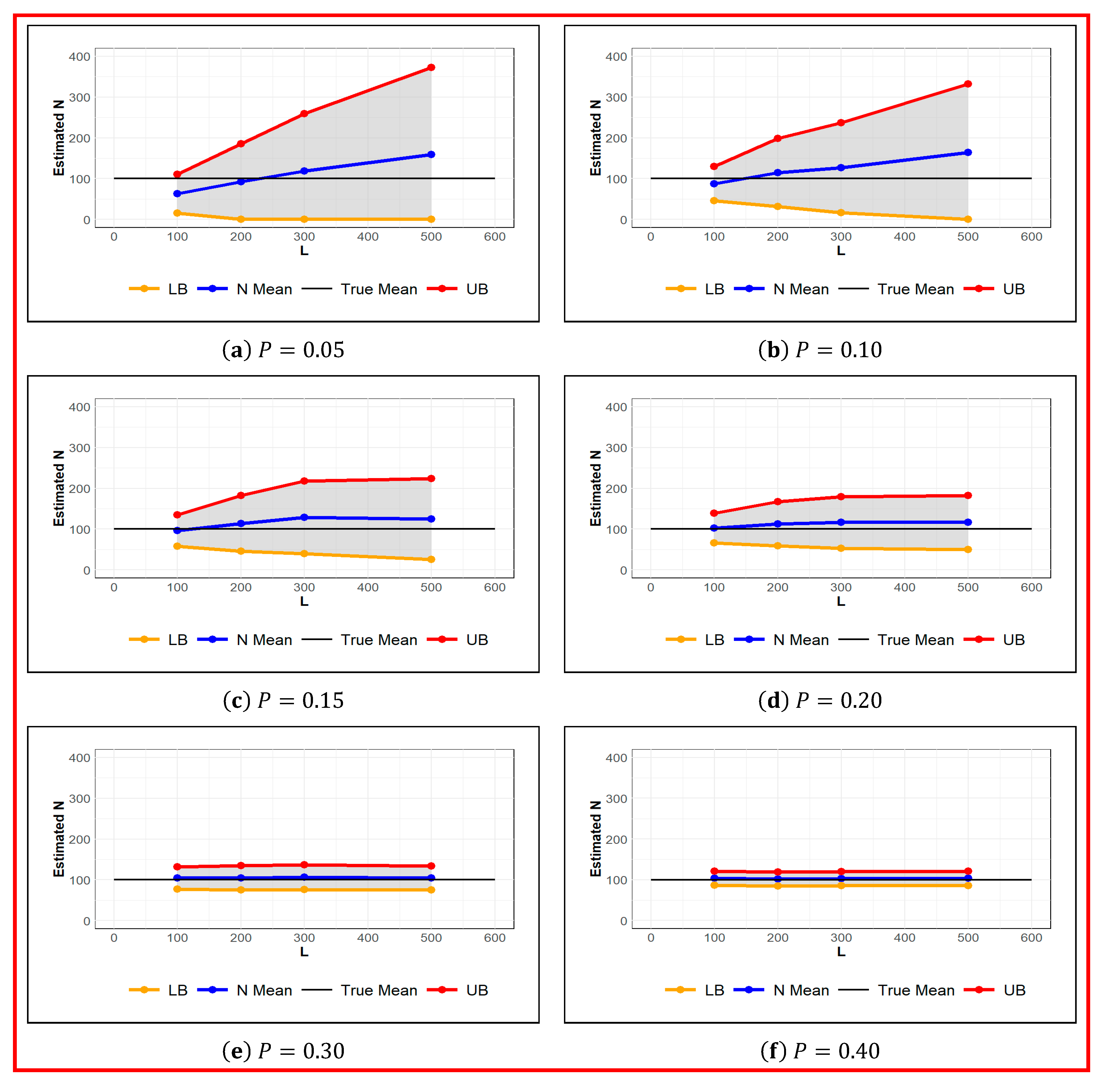
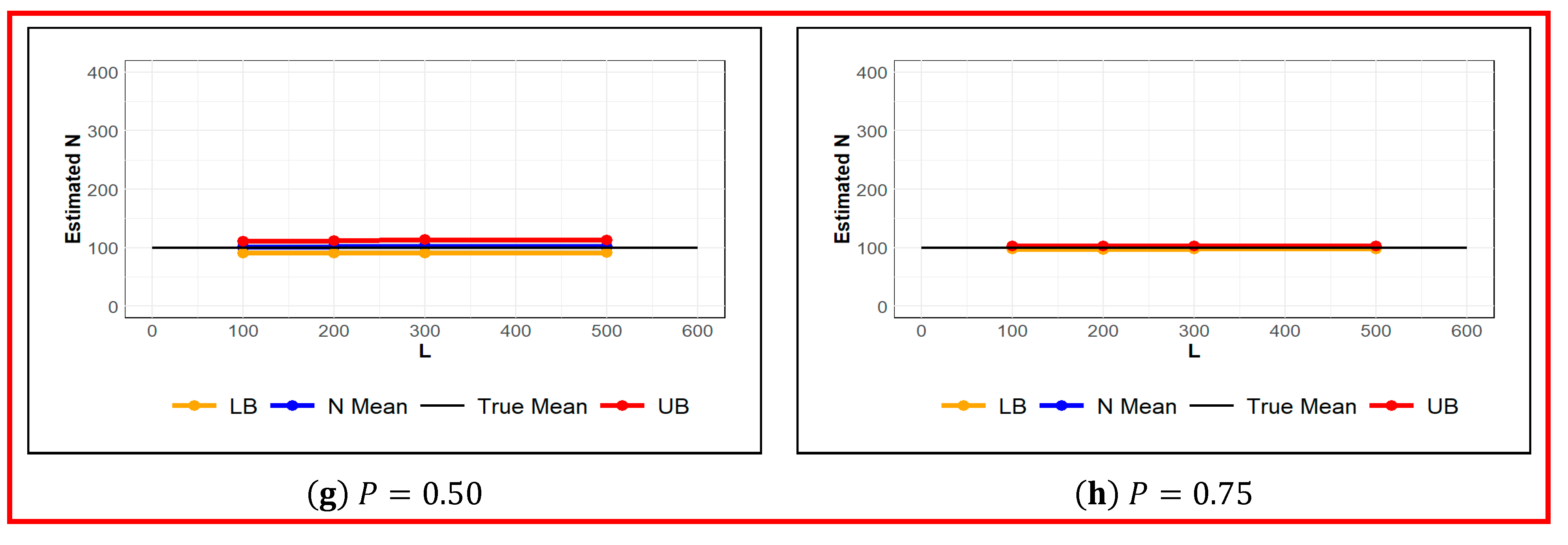
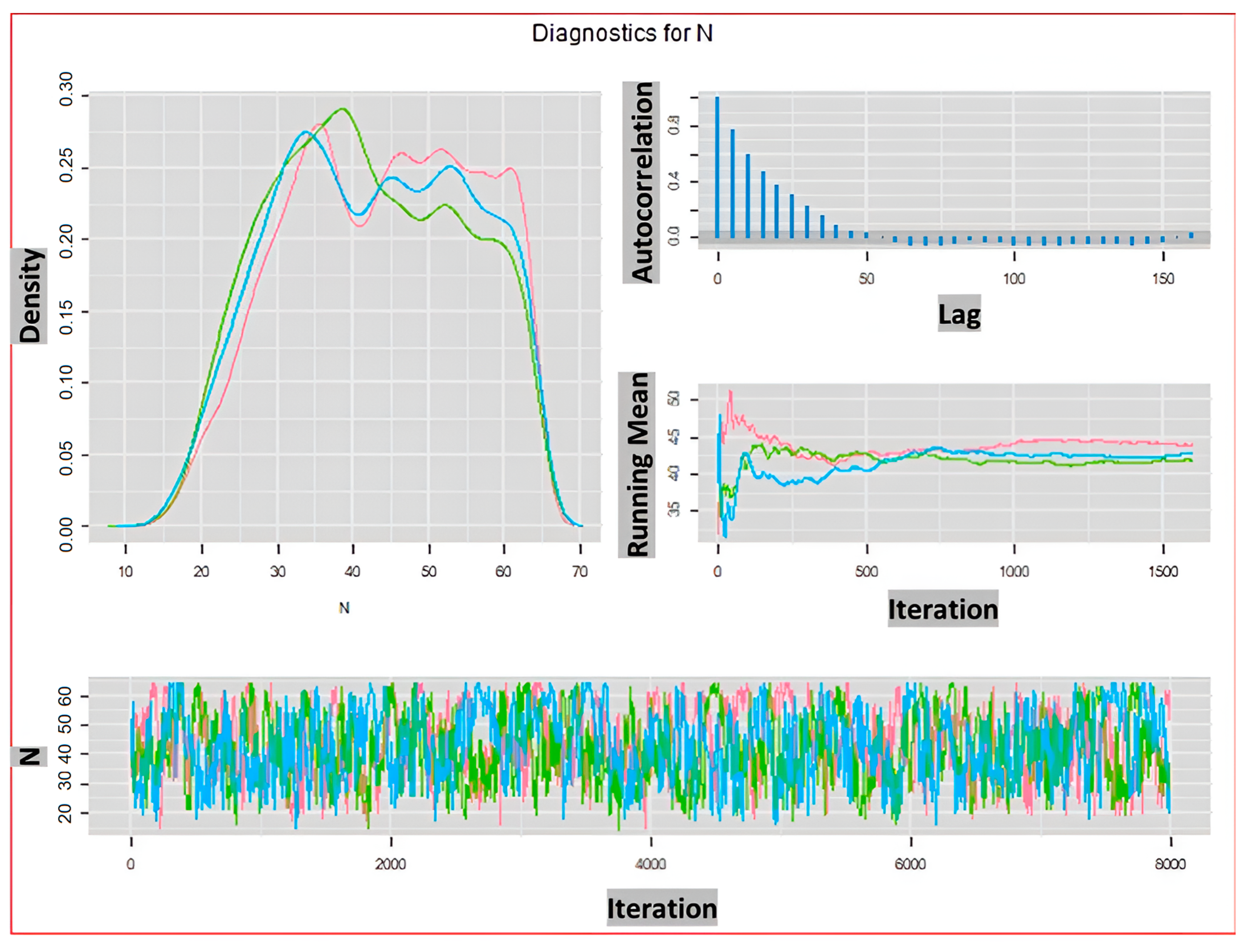
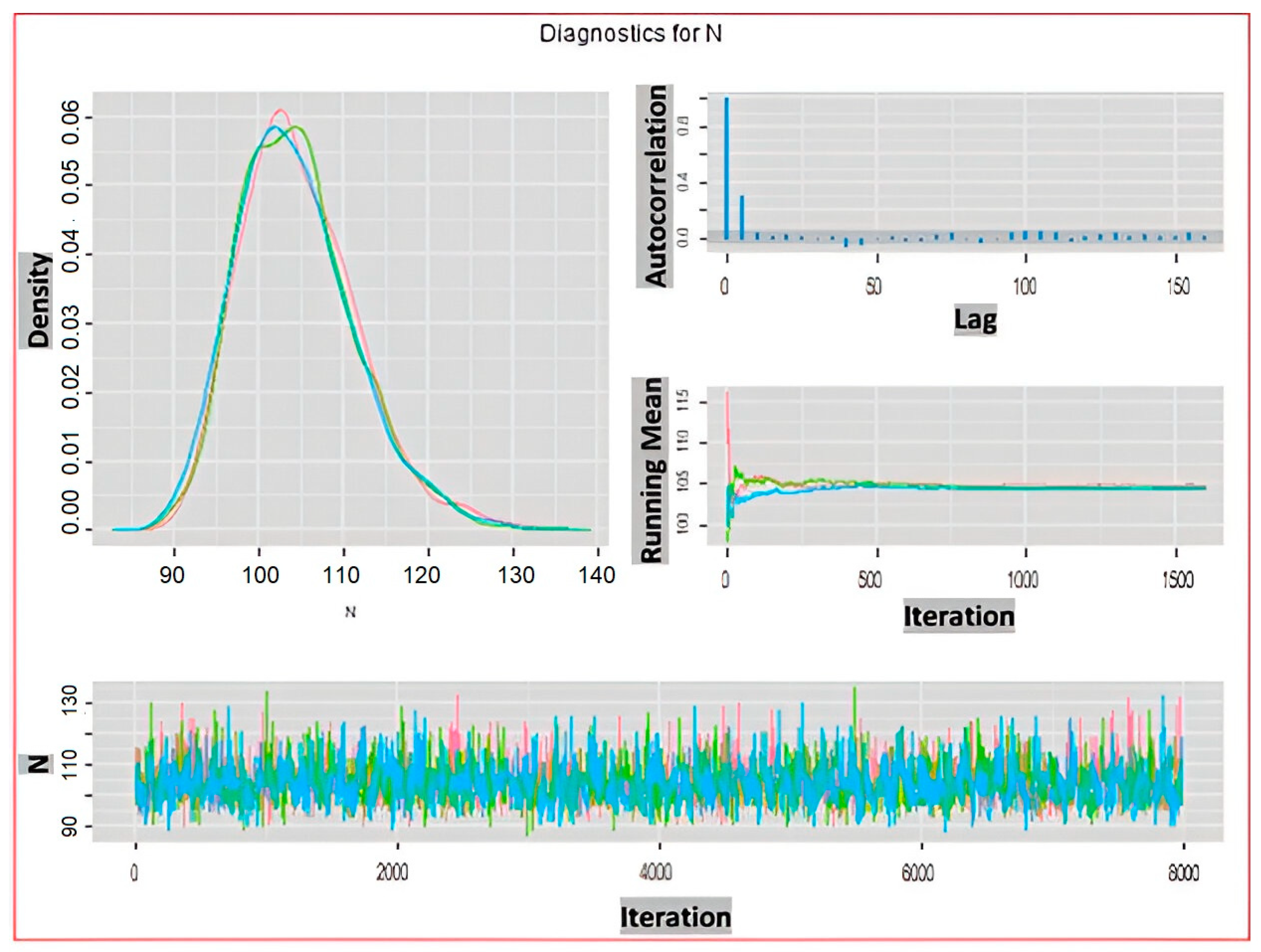
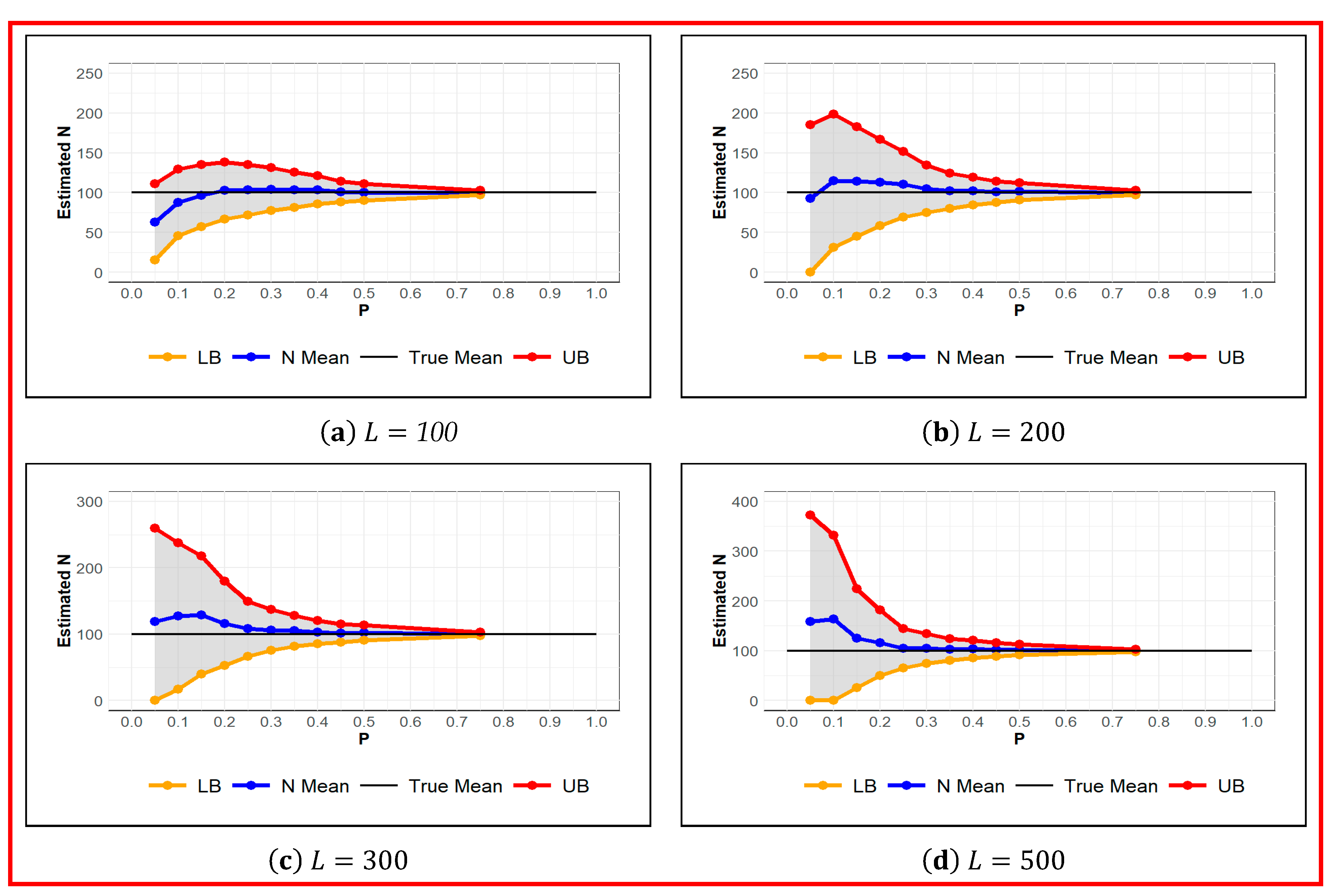
As it is depicted in Figure 1, regardless of the set value for the augmented population parameter, a fair estimate of is obtained for probability of detection of 0.3 or higher. However, based on the estimated values of standard error and the length of confidence interval in Table 1, to achieve an absolute estimation error of 10% or less, the probability of detection should reach 0.5 or higher. The convergence of posterior distributions of and for the probability of detection and are shown in Figure 2 and Figure 3 respectively. We can clearly see in these density plots that Markov chain for converges to almost the same posterior distribution. As it can be observed in Figure 3, all chains are well mixed and the running mean for the first 1500 iterations are almost the same. Moreover, the autocorrelation of the chains for drops considerably faster than that that of .
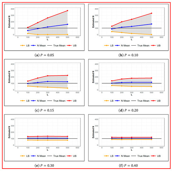
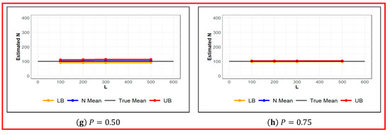
Figure 1.
Estimated for different values of augmented population parameter at set values of probability of detection , given . True (black), Estimated (blue), and Upper and Lower Confidence Bounds (red and orange respectively).
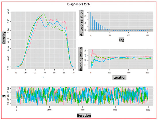
Figure 2.
Diagnostic Plots for estimated with and . Density (top left), Autocorrelation (top right), Ruining mean (middle right), and Trace (bottom). Red, green, and blue show three chains of MCMC.
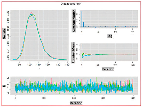
Figure 3.
Diagnostic Plots for estimated with and . Density (top left), Autocorrelation (top right), Ruining mean (middle right), and Trace (bottom). Red, green, and blue show three chains of MCMC.
3.2. Sensitivity of to for Different Values of
Sensitivity of estimated population size is then studied regarding different values for probability of detection at set values of augmented population parameter . As we can see in Figure 4, for , it underestimates the population size for . However, it provides a reasonable and consistent estimate of for . For , it underestimates the population size only for and a satisfactory estimate of is obtained for . For , it overestimates the population size for . The standard error of estimate increases by increasing from 100 to 400. Nevertheless, a standard error of below 10% can be achieved for regardless of value of .
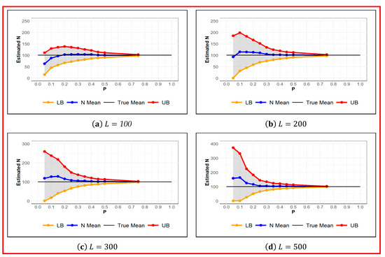
Figure 4.
Estimated for different values of at set values of for given . True (black), Estimated (blue), and Upper and Lower Confidence Interval Limit (red and orange respectively).
3.3. Sensitivity of to for Different Values of
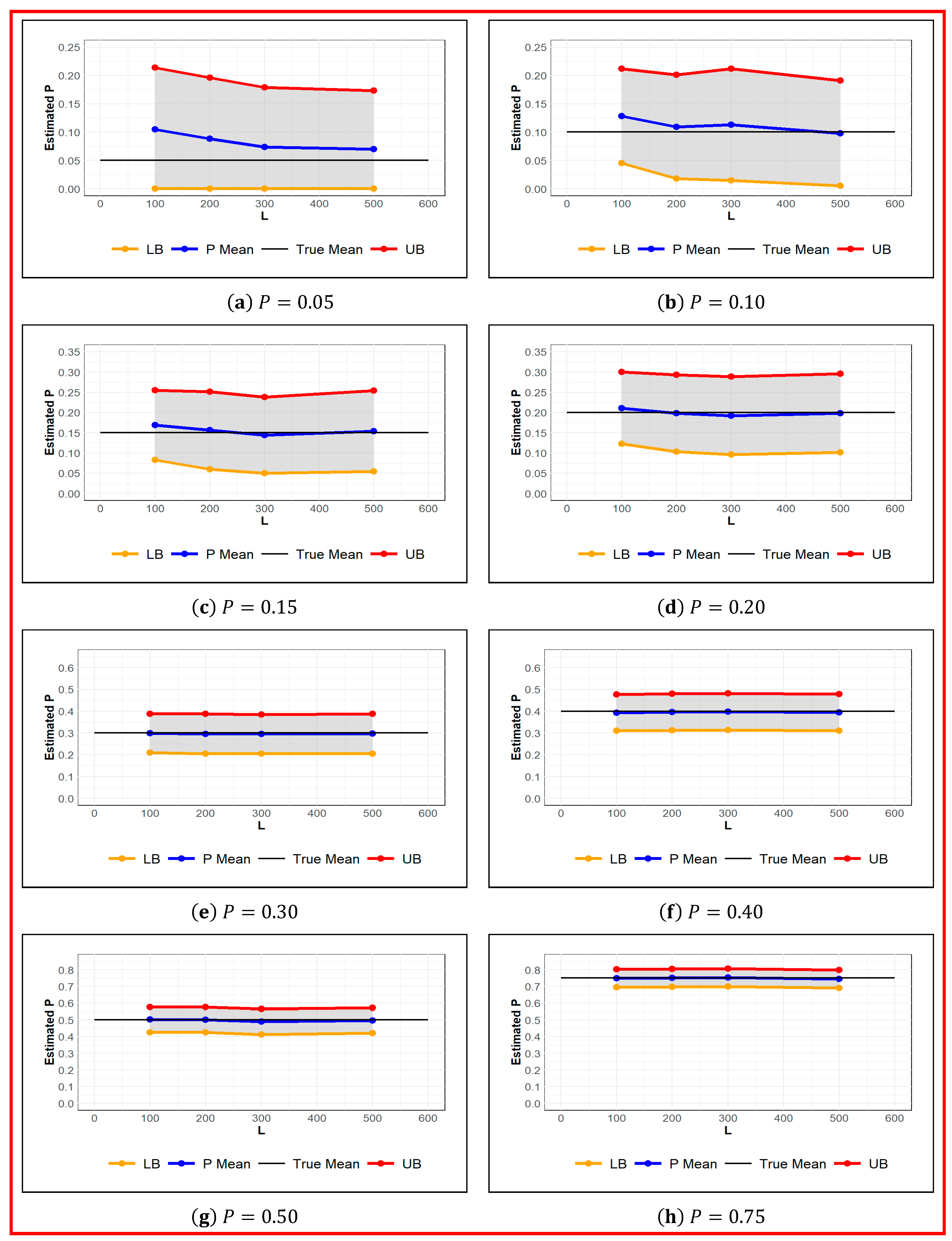
The simulation results demonstrated in Table 2 and depicted in Figure 5, show the estimated value of the probability of detection for different values of augmented population parameter . We can observe that the estimated value of the probability of detection is a fair estimate regardless of given the probability of detection . However, to achieve a standard error of estimate of Overall, the estimated value of the probability of detection is less sensitive to than estimated . Consequently, based on the simulation results, a probability of detection better than 0.25 must be achieved to obtain reliable estimate of the population size . However, to obtain a standard error below 20%, the probability of detection must be 0.4 or higher. Notice that the probability of detection itself is an unknown parameter that depends on the home range of animals. In turn, it is imperative to design the camera grid based on animal home range for sustaining the desired probability of detection .

Table 2.
Estimated Mean of for Different Values of and for Different values of Probability of Detection, along with standard error () and width of credible interval (CI width).
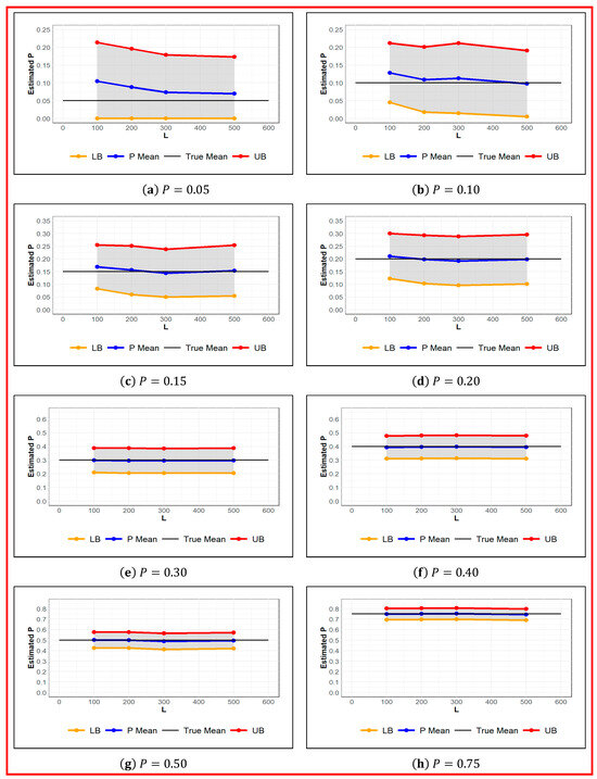
Figure 5.
Estimated Value of for Different Values of at set values of Probability of Detection. True (black), Estimated (blue), Upper and Lower Confidence Interval Limit (red and orange respectively).
3.4. Sensitivity of to for Different Values of
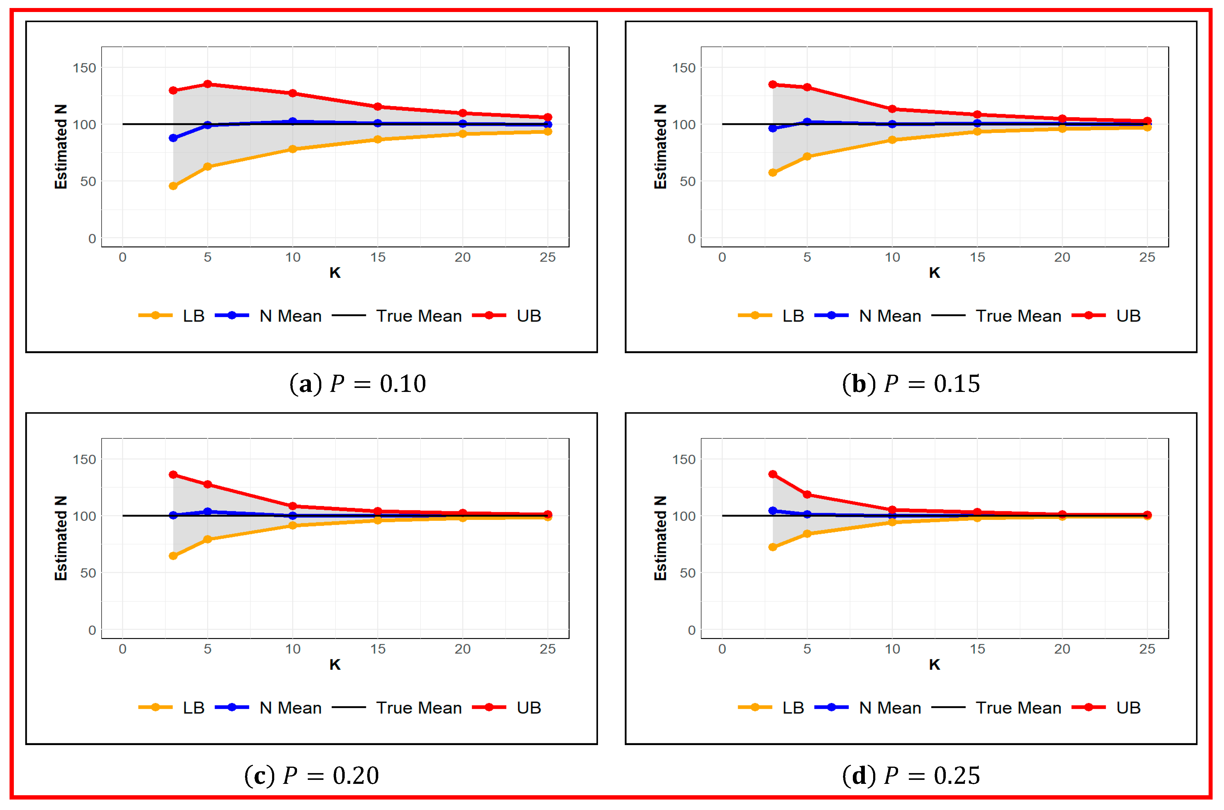
Next, the sensitivity of the estimated population size to the sample size was studied. The sample size depends on the sampling duration or number of occasions. Hence, simulation studies were performed, and the population size and probability of detection were estimated for different number of occasions at set values of probability of detection. From simulation results shown in Table 3 and Figure 6, we can see the impact of the number of occasions on the estimated population size . The estimated ranges from 88 (for and ) to 100 (for and ). Even for small number of occasions (), and low probability of detection (), a reasonable estimate of 88 is obtained. However, the standard error is over 55% for and , and it drops to below 1% for and . Moreover, for a large number of occasions like , the estimated is highly accurate regardless of , such that even for low probability of detection of , the estimation error of is below 7%, while with a moderate probability of detection of , even with , an accurate estimate of with the standard error of below 5% can be achieved. Therefore, if the probability of detection is low, or sufficient information about the abundance of animals is not available, increasing the number of occasions can noticeably improve the accuracy of the estimated population size.

Table 3.
Estimated for Different Number of Occasions and for Different values of Probability of Detection, along with standard error () and width of credible interval (CI width).
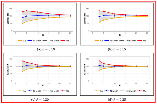
Figure 6.
Estimated Value of for different Number of Occasions for the set values of Probability of Detection . True (black), Estimated (blue), Upper and Lower Confidence Interval Limit (red and orange respectively).
3.5. Sensitivity of to for Different Values of
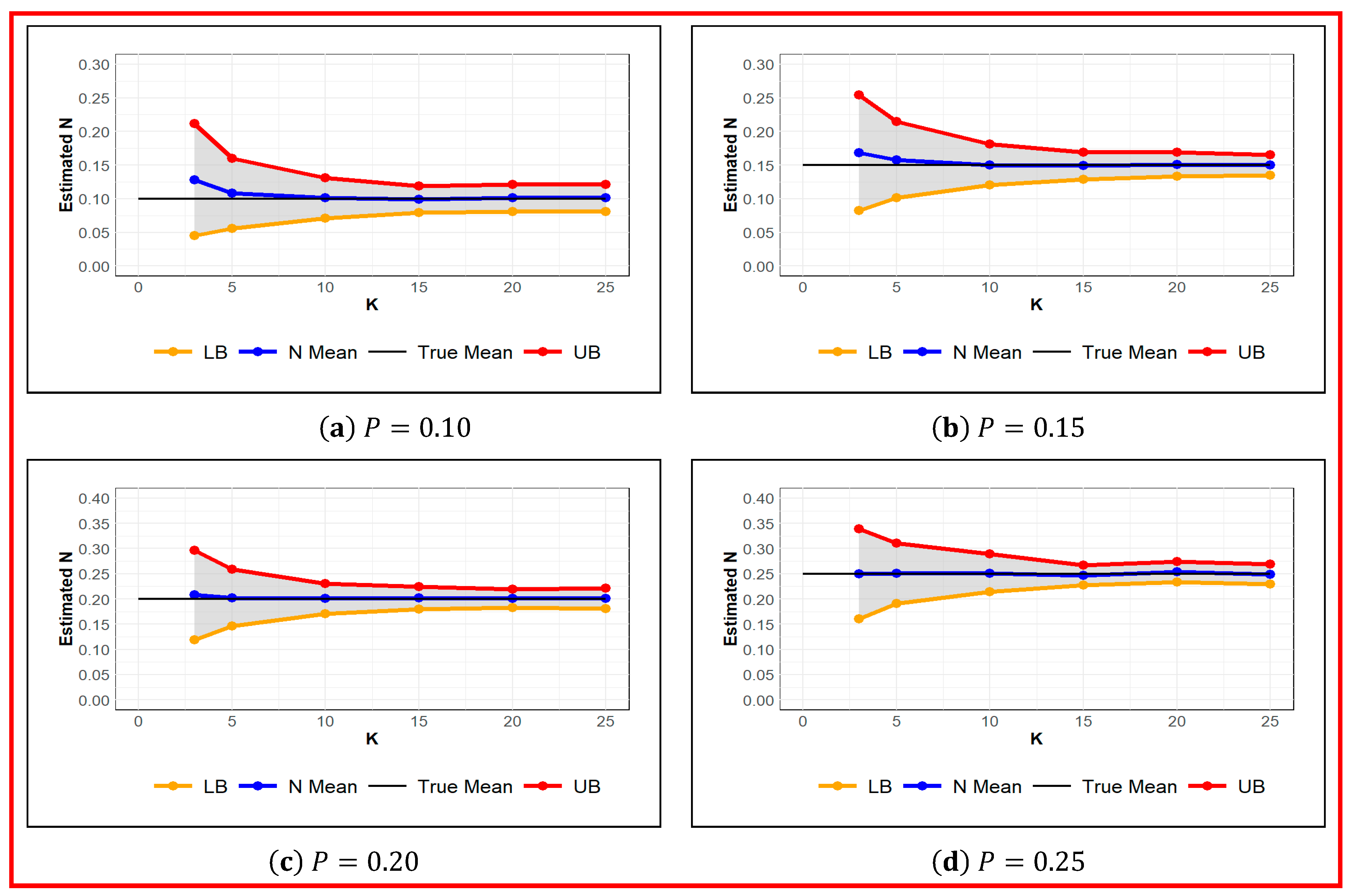
Next, the probability of detection was estimated for different number of occasions at set values of probability of detection. Simulation results in Table 4 and Figure 7 show that the estimated value of the probability of detection is less sensitive to the number of occasions. The absolute error of estimated ranges from zero to 0.028 (or 28%) for and . For a moderate probability of detection of 0.25, the absolute error of is almost zero regardless of the number of occasions. However, with , for a reasonable accuracy with standard error of 15% or higher, must be attained. For a small number of occasions , the standard error ranges from 36% for to 83.5% for . It means even with moderate , if the number of occasions is small (), the estimated has a high standard error. Conversely, with small , a reasonably accurate estimate of with standard error of 15% can be obtained. Therefore, if the probability of detection is low, and/or sufficient information about the abundance of animals is not available, increasing the number of occasions can noticeably improve the accuracy of the estimated population size.

Table 4.
Estimated for Different Number of Occasions and for Different values of Probability of Detections, along with standard error () and width of credible interval (CI width).
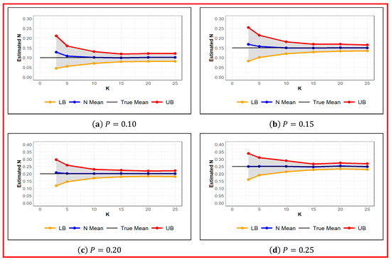
Figure 7.
Estimated Value of for Different values of Probability of Detection and Different Number of Occasions . True (black), Estimated (blue), Upper and Lower Confidence Interval Limit (red and orange respectively).
4. Discussion
The goal of this study was to design a camera grid for stationary wildlife photography to monitor population dynamics. Wildlife population monitoring is essential to manage and control the spatiotemporal variation of population size and density for one or more species. To assess and control a growing population, collected camera encounters will be used to estimate the population size and density. Spatial capture-unmarked, alternatively called capture-unidentified, models are broadly used for population analysis. The sensitivity of these models to the probability of detection was investigated in this study. To do so, unknown probability of detection was sampled using a non-informative prior distribution and randomized camera locations about the center of animals’ home-range. In this way, the likelihood of detecting an individual animal can be calculated using the distance of the camera location from the spatial location of the individual. Hence, the number of cameras and their locations in a camera grid must be carefully chosen to reach an adequate probability of detection based on the random encounters of individual animals with the camera traps.
From the simulation results, it was demonstrated that the standard error of the estimated N depends on the probability of detection. It was verified by simulation that the accuracy of the estimated population size improves by increasing the probability of detection. It was found that a detection probability of at least 0.3 was needed to obtain moderate accuracy for estimating the population size. Furthermore, a standard error of below 10% can be achieved for regardless of value of L. These are notable outcomes of this study which are recommended to ensure a minimum camera coverage for reliable estimation of population size when designing a monitoring system using camera traps.
The estimated population size is also sensitive to the sample size and in turn it depends on the sampling duration. The population size was estimated through numerous simulations with different sampling duration (number of occasions). Yet again, as it was observed for the augmented population parameter L, with a moderate probability of detection , a reasonable estimate of population size can be obtained even with small number of occasions K (shorter sampling duration). It was shown that not only larger values of L could not make up for a poor probability of detection to obtain a reliable estimate of N, but also with a low probability of detection, the accuracy of the estimated N deteriorated by increasing L. In contrast, an accurate estimate of N can be obtained with low probability of detection, contingent on increasing the sampling duration. It was revealed by simulation studies that larger values of K can make up for a poor probability of detection to obtain a reliable estimate of N. Consequently, if the probability of detection is low, or adequate information about the abundance of animals is not available, increasing the number of occasions can noticeably improve the accuracy of the estimated population size.
Here, we studied the impact of detection probability and drove a lower bound for it. However, it must be pointed out that there are several other factors to be considered when designing a camera grid to be able to maintain this recommended lower bound for detection probability for population analysis. There is no single remedy for different scenarios. One such factor is the size of the camera grid, i.e., the number of camera traps utilized and the area that will be surveyed. Because the size of the camera grid has an impact on the detection probability, a sufficient number of cameras is needed in order to achieve the lower-bound detection probability required to obtain an accurate estimate of population size and density [19,20,21].
Another important factor to consider in camera grid design is the placement of the camera traps along specific features, such as roads and trails [21]. There is the potential for significant biases in detection probability with non-random camera trap placements [19,22]. For example, placing camera traps along game trails can significantly increase the detection probability of certain species by up to 33%.
The species being studied must be also considered when designing a camera grid in order to achieve a proper detection probability, as there is significant inter-species variation in detection probability that is influenced by camera trap location [19,23,24]. For example, the number of camera traps required to estimate the population size and density of common species is much smaller than the number of camera traps needed for rare species [20]. A grid where cameras are placed several feet above the ground may capture slow moving or larger species more successfully than faster or smaller species.
Other factors that should be considered for camera trap grid designs are the camera sensing region and the placement of the camera. To meet the lower-bound detection probability, the way an individual is encountered by a camera needs to be considered. In order for an individual to be detected by a camera, that individual must be present in the study area, and it must enter the camera sensing region. This constitutes a true positive detection. However, false positive and negative detections are possible when using camera traps. False positive detections can occur when the camera is triggered but an individual is not present, for example when surrounding vegetation moves by wind or breeze and triggers the motion sensor of a camera. False negative detection occurs when an individual is present in the camera sensing region, but it is not recorded by the camera. In particular false negatives must be considered as they contribute to missing data. This type of detection can occur in many ways, such as when an individual is hidden by the surroundings in the camera sensing region or when an individual passes the camera trap swiftly and is not detected [24]. To reach the recommended lower bound for the detection probability, the false positive and false negative detections must also be taken into account based on the study area [25]. Our future work will be focused to study the sensitivity of the spatiotemporal models to these factors and how these factors can be incorporated into the model to maintain the recommended lower bound for the detection probability.
5. Conclusions
The sensitivity of the model to the augmented population parameter L is more noticeable for low probability of detection. It is important to point out that for low probability of detection , the accuracy of the estimated N decreases with increasing L and the capture-unidentified models tend to noticeably overestimate the population size for large values of the augmented population L. This sounds counterintuitive as it has been recommended to choose large L [14,15] to have accurate estimates of population size. Nevertheless, it was demonstrated in this study that, to maintain reliable estimates of N for large values of L, a probability of detection of or higher must be attained. Moreover, the sensitivity of the estimated N decreases as we increase the probability of detection. Hence, to attenuate the sensitivity of the model to L, a probability of detection of must be reached. Additionally, to obtain a standard error below 15%, the probability of detection of 0.45 or higher must be achieved.
Based on the simulation results, a minimum probability of detection of 0.25 must be attained to obtain consistent estimate of the population size N. However, the probability of detection itself is an unknown parameter due to the random nature of the camera encounters. The probability of detection depends on how often individual animals are captured through camera traps. Consequently, the frequency of the random camera encounters is a function of animal’s home range and its distance from the camera location. Therefore, it is imperative to design the camera grid based on the animal’s home range to attain the desired probability of detection of . Our future work is focused on how to maintain the minimum probability of detection in designing the sampling camera grid.
In the bottom line, we should point out that limited accuracy of the estimated population size [26] is due to intrinsic restrictions of capture-unidentified models. The purpose of this work was to study the sensitivity of capture-unidentified models regarding probability of detection, data augmentation size, and sample size (sampling duration). While it is essential to consider the sensitivity of the model in experiment design to attain a target probability of detection and appropriate sample size, there are other complementary approaches that can potentially improve the estimated population size. Evidently, the implementation of these methods relies on the available resources. For example, marking captured individuals [15] will facilitate their identification, and in turn substantially improves the accuracy of the estimated population size. Another approach to identify the individuals of the population is collecting genetic information using noninvasive methods [27].
Although effective sample size can be quantified in the MCMC method [28], the expected effective sample size must be contemplated during experimental design in association with the probability of detection and augmented population size. In this way, the target probability of detection and appropriate sampling duration can be achieved. Finally, another important aspect of implementing capture-unidentified models using MCMC is the convergence of the Markov Chain [29]. It has been observed in our previous works that the convergence of the Markov Chain (MC) does not necessarily uphold the reliability of the estimated population size [30,31]. Hence, our future research will be conducted to study the sensitivity of MC’s convergence as well as the estimation accuracy of the converged MC, to the augmented population size and the probability of detection.
Author Contributions
Conceptualization, N.N.K.; Methodology, M.J. and N.N.K.; Software, M.J., R.D.B., F.H. and N.N.K.; Validation, M.J., F.H. and N.N.K.; Formal analysis, M.J., R.D.B. and F.H.; Investigation, M.J. and N.N.K.; Resources, N.N.K.; Data curation, R.D.B.; Writing—original draft, M.J., R.D.B., F.H. and N.N.K.; Writing—review & editing, N.N.K.; Visualization, M.J., R.D.B. and F.H.; Supervision, N.N.K.; Project administration, N.N.K. All authors have read and agreed to the published version of the manuscript.
Funding
This research received no external funding.
Data Availability Statement
Data was not collected. The random samples were generated for the simulation studies in this work.
Conflicts of Interest
The authors declare no conflict of interest.
References
- Pollock, K.H. Capture-Recapture Models: A Review of Current Methods, Assumptions and Experimental Design. Available online: https://repository.lib.ncsu.edu/server/api/core/bitstreams/5b4fd48b-48fb-4eba-adf2-1366811bd4f7/content (accessed on 1 January 2023).
- Nichols, J.D. Capture-Recapture Models. BioScience 1992, 42, 94–102. [Google Scholar] [CrossRef]
- Schwarz, C.J.; Seber, G.A. Estimating animal abundance: Review III. Stat. Sci. 1999, 14, 427–456. [Google Scholar] [CrossRef]
- Pollock, K.H. A Capture-Recapture Design Robust to Unequal Probability of Capture. J. Wildl. Manag. 1982, 46, 752–757. [Google Scholar] [CrossRef]
- Pollock, K.H.; Nichols, J.D.; Brownie, C.; Hines, J.E. Statistical Inference for Capture-Recapture Experiments. Wildl. Monogr. 1990, 107, 3–97. [Google Scholar]
- Karanth, K.U. Estimating Tiger Panthera Tigris Populations from Camera-Trap Data Using Capture Recapture Models. Biol. Conserv. 1995, 71, 333–338. [Google Scholar] [CrossRef]
- O’Connell, A.F.; Nichols, J.D.; Karanth, K.U. Camera Traps in Animal Ecology: Methods and Analyses; Springer: Berlin/Heidelberg, Germany, 2011; Volume 271. [Google Scholar]
- Sollmann, R.; Gardner, B.; Belant, J.L. How does spatial study design influence density estimates from spatial capture-recapture models? PLoS ONE 2012, 7, e34575. [Google Scholar] [CrossRef]
- Engeman, R.M.; Massei, G.; Sage, M.; Gentle, M.N. Monitoring Wild Pig Populations: A Review of Methods; USDA National Wildlife Research Center—Staff Publications: Fort Collins, CO, USA, 2013; Paper 1496. [Google Scholar]
- Royle, J.A.; Young, K.V. A Hierarchical Model for Spatial Capture–Recapture Data. Ecology 2008, 89, 2281–2289. [Google Scholar] [CrossRef]
- Royle, J.A.; Karanth, K.U.; Gopalaswamy, A.M.; Kumar, N.S. Bayesian inference in camera trapping studies for a class of spatial capture–recapture models. Ecology 2009, 90, 3233–3244. [Google Scholar] [CrossRef]
- Kery, M.; Gardner, B.; Stoeckle, T.; Weber, D.; Royle, J.A. Use of Spatial Capture-Recapture Modeling and DNA Data to Estimate Densities of Elusive Animals. Conserv. Biol. 2011, 25, 356–364. [Google Scholar] [CrossRef]
- Borchers, D. A non-technical overview of spatially explicit capture–recapture models. J. Ornithol. 2012, 152 (Suppl. S2), S435–S444. [Google Scholar] [CrossRef]
- Royle, J.A.; Chandler, R.B.; Sollmann, R.; Gardner, B. Spatial Capture-Recapture; Academic Press: Cambridge, MA, USA, 2013. [Google Scholar]
- Chandler, R.B.; Royle, J.A. Spatially Explicit Models for Inference About Density in Unmarked or Partially Marked Populations. Ann. Appl. Stat. 2013, 7, 936–954. [Google Scholar] [CrossRef]
- Jaber, M.; Hamad, F.; Breininger, R.D.; Kachouie, N.N. An Enhanced Spatial Capture Model for Population Analysis Using Unidentified Counts through Camera Encounters. Axioms 2023, 12, 1094. [Google Scholar] [CrossRef]
- Royle, J.A.; Dorazio, R.M.; Link, W.A. Analysis of multinomial models with unknown index using data augmentation. J. Comput. Graph. Stat. 2007, 16, 67–85. [Google Scholar] [CrossRef]
- Royle, J.A.; Dorazio, R.M. Parameter-expanded data augmentation for Bayesian analysis of capture–recapture models. J. Ornithol. 2012, 152, 521–537. [Google Scholar] [CrossRef]
- O’Connor, K.M.; Nathan, L.R.; Liberati, M.R.; Tingley, M.W.; Vokoun, J.C.; Rittenhouse, T.A.G. Camera trap arrays improve detection probability of wildlife: Investigating study design considerations using an empirical dataset. PLoS ONE 2017, 12, e0175684. [Google Scholar] [CrossRef]
- Kays, R.; Arbogast, B.S.; Baker-Whatton, M.; Beirne, C.; Boone, H.M.; Bowler, M.; Burneo, S.F.; Cove, M.V.; Ding, P.; Espinosa, S.; et al. An empirical evaluation of camera trap study design: How many, how long and when? Methods Ecol. Evol. 2020, 11, 700–713. [Google Scholar] [CrossRef]
- Hofmeester, T.R.; Cromsigt, J.P.G.M.; Odden, J.; Andrén, H.; Kindberg, J.; Linnel, J.D.C. Framing pictures: A conceptual framework to identify and correct for biases in detection probability of camera traps enabling multi-species comparison. Ecol. Evol. 2019, 9, 2320–2336. [Google Scholar] [CrossRef]
- Kolowski, J.M.; Forrester, T.D. Camera trap placement and the potential for bias due to trails and other features. PLoS ONE 2017, 12, e0186679. [Google Scholar] [CrossRef]
- Mann, G.K.H.; O’Riain, M.J.; Parker, D.M. The road less travelled: Assessing variation in mammal detection probabilities with camera traps in a semi-arid biodiversity hotspot. Biodivers. Conserv. 2015, 24, 531–545. [Google Scholar] [CrossRef]
- Findlay, M.A.; Briers, R.A.; White, P.J.C. Component processes of detection probability in camera-trap studies: Understanding the occurrence of false-negatives. Mammal Res. 2020, 65, 167–180. [Google Scholar] [CrossRef]
- Symington, A.; Waharte, S.; Julier, S.; Trigoni, N. Probabilistic Target Detection by Camera-Equipped UAVs. In Proceedings of the IEEE International Conference on Robotics and Automation, Anchorage, AK, USA, 3–7 May 2010; pp. 4076–4081. [Google Scholar]
- Yamaura, Y.; Kery, M.; Royle, J.A. Study of biological communities subject to imperfect detection: Bias and precision of community N-mixture abundance models in small-sample situations. Ecol. Res. 2016, 31, 289–305. [Google Scholar] [CrossRef]
- Sollmann, R.; Tôrres, N.M.; Furtado, M.M.; Jácomo, A.T.d.A.; Palomares, F.; Roques, S.; Silveira, L. Combining camera-trapping and noninvasive genetic data in a spatial capture–recapture framework improves density estimates for the jaguar. Biol. Conserv. 2013, 167, 242–247. [Google Scholar] [CrossRef]
- Martino, L.; Elvira, V.; Louzada, F. Effective sample size for importance sampling based on discrepancy measures. Signal Process. 2017, 131, 386–401. [Google Scholar] [CrossRef]
- Fabreti, L.G.; Höhna, S. Convergence assessment for Bayesian phylogenetic analysis using MCMC simulation. Methods Ecol. Evol. 2022, 13, 77–90. [Google Scholar] [CrossRef]
- Mohamed, J. A Spatiotemporal Bayesian Model for Population Analysis. Ph.D. Thesis, Florida Institute of Technology, Melbourne, FL, USA, 2022. Available online: https://repository.fit.edu/etd/880 (accessed on 1 January 2023).
- Jaber, M.; Van Woesik, R.; Kachouie, N.N. Probabilistic Detection Model for Population Estimation. In Proceedings of the Second International Conference on Mathematics of Data Science, Old Dominion University, Norfolk, VA, USA; 2018; p. 43. Available online: https://scholar.google.com/citations?user=ghxCwaAeRhoC&hl=en&oi=sra (accessed on 1 January 2023).
Disclaimer/Publisher’s Note: The statements, opinions and data contained in all publications are solely those of the individual author(s) and contributor(s) and not of MDPI and/or the editor(s). MDPI and/or the editor(s) disclaim responsibility for any injury to people or property resulting from any ideas, methods, instructions or products referred to in the content. |
© 2024 by the authors. Licensee MDPI, Basel, Switzerland. This article is an open access article distributed under the terms and conditions of the Creative Commons Attribution (CC BY) license (https://creativecommons.org/licenses/by/4.0/).

