Specification Mining over Temporal Data ^†

Abstract

Current specification mining algorithms for temporal data rely on exhaustive search approaches, which become detrimental in real data settings where a plethora of distinct temporal behaviours are recorded over prolonged observations. This paper proposes a novel algorithm, Bolt2, based on a refined heuristic search of our previous algorithm, Bolt. Our experiments show that the proposed approach not only surpasses exhaustive search methods in terms of running time but also guarantees a minimal description that captures the overall temporal behaviour. This is achieved through a hypothesis lattice search that exploits support metrics. Our novel specification mining algorithm also outperforms the results achieved in our previous contribution.

1. Introduction

Verified artificial intelligence from the perspective of formal methods (Figure 1) concerns the specification, design, and verification of systems represented in mathematical specifications [1]. These all consider a model of the system to be verified $\mathfrak{S}$, a model of the environment $\mathfrak{E}$, and the property to be verified $\mathsf{\Phi }$. When merely focusing on the system to be verified in context-free scenarios, we can also ignore $\mathfrak{E}$ and assume that $\mathfrak{S}$ will contain all the relevant information of interest. The application of such techniques requires the representation of both $\mathfrak{S}$ and $\mathsf{\Phi }$ in a formalism for which efficient decision processes exist, either for verifying the compliance of a system to a specification (formal verification [2], Section 2.3.1) or for producing a system that abides by a given specification (formal synthesis [3,4]). The ability to determine the former also allows us to mine specifications $\mathsf{\Phi }$ from the system represented in our data $\mathfrak{S}$ (specification mining [5], Section 2.3.2). Under these assumptions, formal verification determines whether a system $\mathfrak{S}$ satisfies the property $\mathsf{\Phi }$ through a yes or a no answer ($\mathfrak{S}\vDash \mathsf{\Phi }$). A negative output is accompanied by a counterexample that shows how $\mathsf{\Phi }$ is falsified, while a positive answer also includes a certificate of correctness.

The wide adoption of such techniques makes finding efficient algorithms for solving specification mining tasks more pressing. Relational databases, usually providing more efficient query plans than other NoSQL representations [6], provide suitable representations for storing and querying collections of temporal information, thus including numerical time series [7], temporal updates of entities, and relationships represented in the relational model [8], as well as recording multiple traces as logs. In particular, traces result from observing a completed real-world process, providing a temporally ordered sequence of activities being audited [2,9]. Recent research shows how temporal data can always be represented as traces, as time series segmentations discretise multi-varied time series into discrete, fully observable, linear, and distinct events, identifying the different states in which a system is transiting [10], as well as the variations (increases or decreases) of the values associated with time series [11]. Such a segmentation also allows to optimise pattern searches over temporal processes [10]. In the context of temporal data, long-time proposed declarative languages provide both human-readable representations for temporal behaviours as clauses/templates [12] as well as suitable query languages for expressing formal verification tasks [2,13]. Adopting such languages is extremely beneficial for specification mining tasks, as they fairly restrict the sets of all possible temporal behaviours to certain interesting patterns of interest, thus allowing a restriction of the space search.

Cybersecurity datasets provide ideal use case scenarios for temporal data represented as logs. Those are often represented as a sequence of observable events that are audited while collecting information concerning the attacker’s strategy [2]. As such, sequences are temporal; this makes it the perfect use-case scenario for sequential pattern mining and association rule mining, which then become the basis for attack prediction tasks [14]. This makes them the ideal testbed to verify whether current state-of-the-art specification mining algorithms for temporal data can deal with greater amounts of distinct behaviours and data to be analysed (Section 5.2 vs. Section 5.3). Lagraa et al. [15] show that it is also possible to represent entire malicious log-in sequences as Workflow Nets, a procedural representation of temporal data, mined via sequential process mining algorithms, such as Alpha+++ [16]: Workflow Nets are then used as predictors for malicious log-in attempts through replaying live sequences. Çatak et al. [17,18] also show that it is possible to audit and log malware system call invocations to represent malicious software as a sequence of subsequent instruction invocations. The resulting dataset can then be exploited to train a long short-term memory neural network for distinguishing between eight different types of malware: trojan, backdoor, downloader, worm, spyware, adware, dropper, and virus. The primary distinction between earlier methods and this recent one lies in the resultant specification’s interpretability. While the new approach elucidates the disparities between various malware types post-facto using explainers, such as SHAP [19], the aforementioned approaches inherently extract a white-box classifier. Tools such as Workflow Nets, sequential pattern mining, or association rules deliver explainable results, motivating the rationale behind a specific classification outcome.

Specification mining over logs stipulates the return of temporal behaviour fulfilled by most traces in a log; such a majority constraint is usually assessed through a minimum support threshold $\theta$. This allows the practitioner to impose early stopping conditions to avoid testing underrepresented temporal behaviour. Despite the adoption of such a constraint, state-of-the-art specification mining algorithms [20,21] still test all the traces in the log without using the minimum support threshold as an earlier stopping condition (Section 3.3 and Section 6.3), thus introducing sensible overhead while testing unnecessary temporal behaviour. This is a desired feature when dealing with real data. Furthermore, the aforementioned approaches are hindered by the exhaustive generation and testing of declarative clauses instantiated over each frequently occurring event type [20,21], thus being heavily hindered by the curse of propositionalisation. As a result, existing approaches do not adequately scale up to the size of big and real-world datasets, as the running time becomes quite explosive in the long run (Section 5.3). As the adoption of a declarative language to express the temporal behaviour of interest considerably reduces the space search for the temporal behaviour to be returned as a specification, we can efficiently visit our search space by organising the candidate’s temporal behaviour to be tested as a lattice (Section 2.2 and Section 4.3), where the descent is pruned using the aforementioned $\theta$ as an early stopping condition. As a consequence of the missed opportunity to exploit faster search approaches, current algorithms do not ensure the provision of specifications of compact sizes. This feature is essential due to the profusion of mined declarative clauses which are later utilized as features to describe temporal data sequences in learning tasks [21] (Section 2.1). Such an approach can easily lead to trained models that overfit the training dataset [22], while training data with such an explosive amount of features requires an exponential number of data samples with respect to the number of such features (https://youtu.be/QZ0DtNFdDko, accessed on 10 September 2023).

This paper proposes Bolt2, an extension of our previous specification mining algorithm Bolt [5], which improves the former in terms of specification size reduction, providing a comparable running time to our initial solution. Our controlled experiments show that our heuristic algorithm can find the most specific behaviour with the best support if compared to other algorithms returning all the possible clauses (Section 5.1), while adopting a general-to-specific lattice search to traverse the declarative clause space, combined with pruning and heuristic assumptions for inference, the algorithm significantly surpasses existing exhaustive search methods. This makes it ideal for mining data-sparse real-world temporal datasets (Section 5.2 and Section 5.3). As any mined specification can then be decomposed into minimal features to be fed to a classifier, we postulate that an ideal specification mining algorithm for temporal data shall return a minimal specification that “adequately” describes the temporal data of interest.

2. Related Work

In this section, we use the notation from [23] for uniformly describing data mining and machine learning problems.

2.1. Machine Learning

Machine learning studies systems that enhance their behaviour over time through experience. This experience consists of a set of examples ${\mathcal{L}}_e$ in which we look for regularities or patterns fitting a specific model. Such a set of examples might be labelled with a $f:{\mathcal{L}}_e\to \mathcal{Y}$ function, associating each example to a target classification class $y\in \mathcal{Y}$. We can, therefore, define a (labelled) dataset as a collection of pairs $D=\left\{({\mathbf{x}}_0,y_0),\dots ,({\mathbf{x}}_{m-1},y_{m-1})\right\}$, associating each data point ${\mathbf{x}}_i$ to a class $f\left({\mathbf{x}}_i\right)=y_i\in \mathcal{Y}$. We can define the set of all the possible training outcomes (i.e., hypotheses) as ${\mathcal{L}}_h:={\mathcal{Y}}^{{\mathcal{L}}_e}\equiv \left\{h|h:{\mathcal{L}}_e\to \mathcal{Y}\right\}$, among which, we are interested in a function $\tilde{f}$ that minimises the classification loss when compared to the expected output f. The training problem can then be summarised as follows:

$$ML(\mathit{loss},D,{\mathcal{L}}_h):=\underset{h^{\prime }\in {\mathcal{L}}_h}{arg\; min}\mathit{loss}(h^{\prime },D)$$

When using decision trees [24] as use case examples for explainable machine learning models, each path $\pi :=r\to p_1\to \cdots \to l_n^y$ from the root r toward a leaf $l_n^y$ node associated with a class $y\in \mathcal{Y}$ describe a classification rule $r\wedge {\bigwedge }_{p_i\in \pi }{p}_i\Rightarrow y$, where each predicate might be (or might not be) negated, depending on the direction followed while traversing the learned model. As each branch provides alternative specifications for a class, we can extract an explanation for each class $y\in \mathcal{Y}$ as a finitary disjunction of all the rule tails associated with the same head y.

Deviant model learning (DML) [21] generates specifications (a.k.a. models) that uniquely characterise classes of traces present in a log through a mixture of declarative and procedural (i.e., patterns) features that are mined from the data (Section 2.2). It assumes that the log associates each trace $\sigma$ to a specific class $y_{\sigma }\in \mathcal{Y}$. As the authors represent the presence/absence of a feature in a trace $\sigma$ as a number ${\overrightarrow{x}}_{\sigma }$[ℓ], each trace can be represented as an n-dimensional embedding ${\overrightarrow{x}}_{\sigma }\in {\mathbb{R}}^n$, where n is the overall number of features, e.g., when a Declare clause c_ℓ is chosen as the ℓ-th feature, a value of ${\overrightarrow{x}}_{\sigma }$[ℓ]$=-1/0/n$ denotes that the trace $\sigma$ does not satisfy, vacuously satisfies, or  satisfactorily activates c_ℓ n times. For the features providing declarative characterisations, DML extracts those via the ADM+Specification mining algorithm [21] (Section 2.3.2). Any improvement in the specification mining phase ensuring model minimality will also minimise both the risk of model overfitting and the curse of dimensionality, as discussed in the introduction of this paper. Therefore, we aim to improve the preliminary mining phase before effectively discussing how to cope with the learning phase, which will be part of our future contribution. As the experiments in this paper are biased toward learning descriptions of deviant specifications expressed as conjunctive declarative clauses, no evidence of the possibility of returning specifications in disjunctive normal form is provided.

2.2. Data Mining

Contrary to machine learning algorithms, data mining algorithms do not limit themselves to the provision of one single hypothesis as they rather return all hypotheses that satisfy a quality criterion $\mathcal{Q}$. Given $h\in {\mathcal{L}}_h$ and two classes $\mathcal{Y}=\mathbf{2}\equiv \{0,1\}$, we can define a cover function $\mathbf{co}(h,D)=\{x\in D|h\left(x\right)=1\}$ as the function identifying the set of all items that are covered by the hypothesis h from D. Data mining algorithms are often interested in returning only the hypotheses exhibiting frequent patterns. We can then define the minimum frequency criterion over a minimum threshold $\theta$ as follows:

$${\mathcal{Q}}_{\theta }(h,D):=\left|\mathbf{co}(h,D)\right|\ge \theta$$

We capture all possible data mining algorithms with the following mathematical formulation:

$$DM(\mathcal{Q},D,{\mathcal{L}}_h):=\{h\in {\mathcal{L}}_h|\mathcal{Q}(h,D)\mathrm{holds}\}$$

Under the previous assumptions, one natural way to structure the hypothesis search space is to employ a generality relation ⪯. We state that a hypothesis $h_2$ is more general than $h_1$ if all the examples covered by $h_1$ are also covered by $h_2$, expressed as

$$h_2⪯h_1\iff \mathbf{co}(h_1,D)\subseteq \mathbf{co}(h_2,D)$$

Despite the exhaustive generation of all possible hypotheses in ${\mathcal{L}}_h$ satisfying $\mathcal{Q}$ being inefficient (Algorithm 1), we can enhance efficiency by pruning the majority of non-valid hypotheses. For binary classification problems, the set of all possible hypotheses is ${\mathbf{2}}^{{\mathcal{L}}_e}$, so each possible predicted positive example in $\wp \left({\mathcal{L}}_e\right)$ represents the outcome of one single hypothesis. Given that there is an isomorphism between the set of hypotheses and the set of all possible data subsets $\wp \left({\mathcal{L}}_e\right)$ (Lemma A1 in Appendix A), we can directly search the hypotheses by navigating the lattice space by ⪯ using a general-to-specific visit. After proving that all the generalisations of hypotheses will satisfy the same quality criterion when a minimum-frequency ${\mathcal{Q}}_{\theta }$ is used (Lemma A2), it follows, by duality, that none of the specialized hypotheses not meeting this criterion will satisfy it either.

Algorithm 1 Brute-force hypothesis generation [23]

1: function Enumerate($\mathcal{Q},D,{\mathcal{L}}_h$) 2:     $\mathtt{H}\leftarrow \varnothing$ 3:     for all $h\in {\mathcal{L}}_h$ do if $\mathcal{Q}(h,D)$ then $\mathtt{H}\leftarrow \mathtt{H}\cup \left\{h\right\}$ 4:     return H

While simplistic mining algorithms [20,21,25] enumerate and test all possible hypotheses in ${\mathcal{L}}_h$ (Algorithm 1), more efficient ones [5,26,27] represent the whole hypothesis space as a lattice induced by the ⪯ relationship while traversing from the most general hypothesis (⊤, Algorithm 2 Line 2) toward the most specific ones, while still validating the quality conditions, which are then returned (Line 7). These last solutions require the definition of a specialization operator $\rho$. This operator associates a hypothesis with all other hypotheses that are less general than itself, formulated as $\rho \left(h\right)=\{h^{\prime }\in {\mathcal{L}}_h|h⪯h^{\prime }\}$ (Line 8). For frequent pattern mining, specialisation involves the extension of the set with a new frequent item [26]. For multi-dimensional frequent sub-graph mining, the specialization entails either the specialization of the nodes appearing in a graph pattern with more specific terms according to a taxonomy [27] or the extension of the graph with further edges and nodes [28]. We can always slightly refine this algorithm to return the S-border containing maximally specific solutions within a data mining solution, thus returning the most specific hypotheses that still satisfy the quality criterion:

$$max\left(\mathit{DM}(\mathcal{Q},D,{\mathcal{L}}_h)\right)\mathrm{where}max\left(T\right)=\left\{h\in T|\nexists t\in T.h\prec t\right\}$$

With respect to temporal model mining from linear finite logs of finite traces $\mathfrak{S}$, our previous contribution defined a specialization $\rho$ for declarative dataless clauses through logical entailment [5]. With respect to this, our current contribution relies on a more solid theoretical foundation related to the adequacy of our quality criterion of choice (Section 3.4) and some improved branch-and-bound heuristic conditions (Section 3.3); it is adopted to fasten the search while making more refined assumptions about the data (Section 6.3). To ensure specification size reduction, our aim is to return the S-borders of such clauses rather than return all clauses with different support types that do not use max as a post-processing operator, as in [20]. Moreover, we intend to design a quality criterion. This criterion will ensure that the most refined candidate neither compromises the support of any more general clause nor falls below a specified minimum support threshold.

Algorithm 2 General-to-specific lattice search [23]

1: function GeneralToSpecific${}_{\top \in {\mathcal{L}}_h,\rho }$($\mathcal{Q},D,{\mathcal{L}}_h$) 2:     Queue ⟵ {⊤} 3:     H ⟵ ∅ 4:     while Queue ⟵ ≠ ∅ do 5:         h ⟵ pop(Queue) 6:         if $\mathcal{Q}${h,D} then 7:             H ← H ∪ {h} 8:             Queue ← Queue ∪ ρ (h) 9:         end if 10:    end while 11:    return H

2.2.1. Frequent Pattern Mining

Given a set of all possible transactions T, and a set of occurring items $I={\bigcup }_{t\in T}t$, an itemset is an element of $i\in \wp \left(I\right)$. Support $\varsigma \left(i\right)$ of any itemset i is defined as the ratio between the number of transactions T being supersets of i and the total number of transactions. Given a minimum support threshold $\theta$, an item i is frequent if its support is greater or equal to $\theta$. We can express the representativeness of an itemset in the whole set of transactions as a frequency metric ${\varsigma }^{\prime }\left(i\right)$ defined as the number of traces where i appears:

$${\varsigma }^{\prime }\left(i\right)=|\left\{t\in T|i\subseteq t\right\}|$$

(1)

We denote $\varsigma$ as the normalisation of such support by providing a ratio between ${\varsigma }^{\prime }\left(i\right)$ and the overall number of available transactions $\left|T\right|$.

We focus our attention on two frequent itemset mining algorithms. The Apriori [25] is a brute-force mining algorithm that begins by calculating an ${\mathbf{F}}_1$ table, which associates each item in I with its support, denoted as ${\varsigma }^{\prime }\left(i\right)$. For each i-th iteration step from 1 to $\left|I\right|$, the algorithm prunes each frequent itemset table ${\mathbf{F}}_i$ containing all of the itemsets of length i using a minimum-support threshold $\theta$. If ${\mathbf{F}}_i$ is not empty, we might compute the itemsets of length $i+1$ as ${\mathbf{F}}_{i+1}:={\mathbf{F}}_1\times {\mathbf{F}}_i$. In the worst-case scenario, this algorithm runs in exponential time: $O\left(2^{\left|I\right|}\right)$. FP-Growth [26] improves the time complexity of the former algorithm by merging the itemset generation phase with the itemset pruning via the minimum support threshold, considerably reducing the overall time complexity. This enhancement exploits an item support table and the representation of frequent patterns as a prefix tree. The latter guarantees a compact in-memory representation of the transactions, and offers an efficient general-to-specific approach when generating frequent candidate itemsets.

2.2.2. Association Rule Mining

An association pattern [29] $X\to Y$ states that “if X occurs in the current transaction $t\in T$, then it is likely that Y will occur, too”. We refer to X as the antecedent or tail and to Y as the consequence or head. Each frequent itemset Z can be considered as a rule $\varnothing \to Z$, stating that Z is a possible configuration within our dataset. Association rule mining can be generalised through general-to-specific algorithms [23], refining each possible frequent itemset i expressed as $\varnothing \to i$ to the set of all possible rules $X\to Y$, where $X\cup Y=i$ and $X\cap Y=\varnothing$. In particular, if we perform this for each itemset, we obtain a correct confidence-based pruning algorithm [29] by visiting the lattice of all possible rules descending from i, where $\varnothing \to i$ ($i\to \varnothing$) is its top (bottom). Support and confidence metrics quantify the strengths of such rules from different perspectives. Support s determines how often a rule is “applicable” to the transactions in T, while confidence c determines how frequently items in Y appear in “transactions containing X”. These can be defined as follows:

$$s(\mathsf{X}\to \mathsf{Y})=\frac{{\varsigma }^{\prime }\left(X\cup Y\right)}{\left|T\right|}c(\mathsf{X}\to \mathsf{Y})=\frac{{\varsigma }^{\prime }\left(X\cup Y\right)}{{\varsigma }^{\prime }\left(X\right)}$$

(2)

2.3. Verified Artificial Intelligence for Temporal Data

The present paper concerns specification mining for temporal data, where properties to be verified $\mathsf{\Phi }$ are expressed in linear time logic for finite traces (LTL_f) or the extensions. The LTL_f formalism [3] extends modal logic to include linear, discrete, and future-oriented time, where each event represents a single relevant instant of time. LTL_f quantifies only on events reported in the trace, so each event of interest is fully observable, as the events represented in each trace are totally ordered. The syntax of a well-formed LTL_f formula $\varphi$ is defined as follows:

$$\varphi ::=\mathtt{a}|\neg \varphi |\varphi \vee {\varphi }^{\prime }|\varphi \wedge {\varphi }^{\prime }|{\displaystyle ◯}\varphi |\square \varphi |\diamond \varphi |\varphi \mathcal{U}{\varphi }^{\prime }$$

(3)

where $\mathtt{A}\in I$ represents an atomic proposition, $◯\varphi$ determines that the condition $\varphi$ must hold from the subsequent temporal step, $\square \varphi$ requires that such a condition must always hold from the current instant of time, $\diamond \varphi$ specifies that the current condition must happen at any time in the future, and $\varphi \mathcal{U}{\varphi }^{\prime }$ shows that $\varphi$ must hold until the first occurrence of ${\varphi }^{\prime }$ does. The remainder are interpreted as classical logical connectives, where the implication connective $\varphi \Rightarrow {\varphi }^{\prime }$ can be interpreted as $\neg \varphi \vee (\varphi \wedge {\varphi }^{\prime })$ [30]. The semantics are usually defined in terms of the first-order logic [3] for a given trace ${\sigma }^i$ at a current time j (e.g., for event ${\sigma }_j^i$).

Under the LTL_f framework, any given event in a sequence of interest is immediately followed by a single possible future event. This enforces a specific representation of systems, denoted as $\mathfrak{S}$, as a collection of sequences of distinguishable events ${\sigma }^i\in \mathfrak{S}$ (i.e., a trace) [2]. Each trace ${\sigma }^i$ is a temporally ordered and finite sequence of distinct events ${\sigma }^i={\sigma }_1^i\cdots {\sigma }_n^i$. Each event ${\sigma }_j^i=\langle {\mathtt{A}}_j^i,{\delta }_j^i\rangle$ pairs an activity label ${\mathtt{A}}_j^i\in I$, describing the specific actions performing/occurring in a given event, a payload ${\delta }_j^i$, and a finite function mapping each key to a single value. In this context, the formal verification determines which traces in a log satisfy an LTL_f formula [2] while formal synthesis concerns the generation of traces abiding by an LTL_f formula [4].

A transaction $t\in T$ differs from the trace representation $\sigma$; the former presents items in the form of sets, and the latter captures a sequence of temporally ordered events. Events might still be represented as items through their associated activity labels; therefore, I denotes the set of all activity labels. The conversion of a trace to a transaction comes at the cost of losing temporal information.

2.3.1. Formal Temporal Verification

In the context of LTL_f and temporal data, a counterexample of temporal verification is usually expressed as a non-empty edit sequence for a specific trace invalidating $\mathsf{\Phi }$, thus showing which events have to be removed or added to make a trace compliant to $\mathsf{\Phi }$ [31]. On the other hand, the certificate of correctness associated with traces often reflects the association between the atomic propositions in the formula and the events satisfying such conditions [2,30], and are often referred to as activation B, target B, and correlation $\mathsf{\Theta }$ conditions (see the following paragraph). As the present paper focuses on positive specification mining, we are only going to consider the latter aspect.

‘Declare’ [12] expresses properties $\mathsf{\Phi }$ as conjunctions of clauses providing a specification (or model) $\mathsf{\Phi }$, where each clause is an instantiation of a specific temporal template. A Declare template differs from customary association rules as the latter enforces no temporal occurrence pattern between the conditions at the head and the tail of the rule. Declare can be assessed over a finite multiset of finite traces.

Templates express abstract parameterised temporal properties (first column of  

Table 1. A set of dataless Declare templates considered in the paper. The clauses are marked according to their implementations in the respective Bolt/Bolt2 algorithmic implementations. Surround is our novel clause that, to the best of our knowledge, was first introduced in this paper. To simplify the characterisation of such clauses, we always assume that the first argument of the clause provides its activation A, while the second argument always provides a target B or an alternative activation A’.

Exemplifying Clause (${\mathit{c}}_{\mathit{l}}$)	Natural Language Specification for Traces	LTLf Semantics ($〚{\mathit{c}}_{\mathit{l}}〛$)	Bolt	Bolt2
Init(A)	The trace should start with an activation	A	✓	✓
End(A)	The trace should end with an activation	$Last\left(A\right)$	✓	✓
Exists($A,n$)	Activations should occur at least n times	$\left\{\begin{array}{cc}\diamond (A\wedge ◯(〚\mathsf{Exists}(A,n-1)〛\left)\right)\hfill & n>1\hfill \\ \diamond (A\wedge p)\hfill & n=1\hfill \end{array}\right.$	✓	✓
Absence($A,n+1$)	Activations should occur at most n times	$\neg 〚\mathsf{Exists}$($A,n+1$)〛	✓	✓
Choice($A,A^{\prime }$)	At least one of the two activation conditions must appear.	$\diamond A\vee \diamond A^{\prime }$	✓	✓
ExclChoice($A,A^{\prime }$)	Only one activation condition must happen.	$〚\mathsf{Choice}(\mathtt{A},{\mathtt{A}}^{\prime })〛\wedge 〚\mathsf{NotCoExistence}(\mathtt{A},{\mathtt{A}}^{\prime })〛$	✓	✓
RespExistence($A,B$)	The activation requires the existence of the target.	$\diamond A\Rightarrow \diamond B$	✓	✓
CoExistence($A,B$)	RespExistence, and vice versa.	$〚\mathsf{RespExistence}(\mathtt{A},\mathtt{B})〛\wedge 〚\mathsf{RespExistence}(\mathtt{B},\mathtt{A})〛$	✓	✓
Precedence($A,B$)	Events preceding the activation should not satisfy the target	$\neg B\mathcal{W}A$	✓	✓
ChainPrecedence($A,B$)	The activation is immediately preceded by the target.	$\square (◯\square A\Rightarrow B)$	✓	✓
Response($A,B$)	The activation is either followed by or simultaneous to the target.	$\square (A\Rightarrow \diamond B)$	✓	✓
ChainResponse($A,B$)	The activation is immediately followed by the target.	$\square (A\Rightarrow ◯B)$	✓	✓
Succession($A,B$)	The target should only follow the activation.	$〚\mathsf{Precedence}(\mathtt{A},\mathtt{B})〛\wedge 〚\mathsf{Response}(\mathtt{A},\mathtt{B})〛$	✗	✓
ChainSuccession($A,B$)	Activation immediately follows the target, and the target immediately precedes the activation.	$〚\mathsf{ChainPrecedence}(\mathtt{B},\mathtt{A})〛\wedge 〚\mathsf{ChainResponse}(\mathtt{A},\mathtt{B})〛$	✗	✓
Surround($A,B$)	The activation is immediately followed by, and immediately preceded by, the target.	$〚\mathsf{ChainPrecedence}(\mathtt{A},\mathtt{B})〛\wedge 〚\mathsf{ChainResponse}(\mathtt{A},\mathtt{B})〛$	✗	✓

), where semantics can be expressed in terms of the LTL_f (third column). The provided definitions align with the prevailing literature’s interpretations, subject to $\alpha$-renaming (Section 6.4). We assert that a trace ${\sigma }^i$ satisfies a Declare clause c if it meets the associated semantic representation in LTL_f; we denote this as ${\sigma }^i\vDash \left[\left[c\right]\right]$. We also state that a trace conforms to a (conjunctive) Declare specification (or model) if the trace satisfies each of the clauses $\mathsf{\Phi }={\left\{c_l\right\}}_{l\le n,n\in \mathbb{N}}$ composing the aforementioned specification, i.e., ${\sigma }^i\vDash \mathsf{\Phi }\iff {\sigma }^i\vDash {\bigwedge }_{c_l\in \mathsf{\Phi }}\left[\left[c_l\right]\right]$. This verification process is also referred to as conformance checking in the business process management literature. We also state that an LTL_f formula $\varphi$ implies ${\varphi }^{\prime }$ if all the traces satisfying the former also satisfy the latter. We denote this as $\varphi \Rightarrow {\varphi }^{\prime }$, where we state that ${\varphi }^{\prime }$ is more general than $\varphi$ by interpreting the coverage set as the set of all traces in the log satisfying a given declarative clause (Lemma A3).

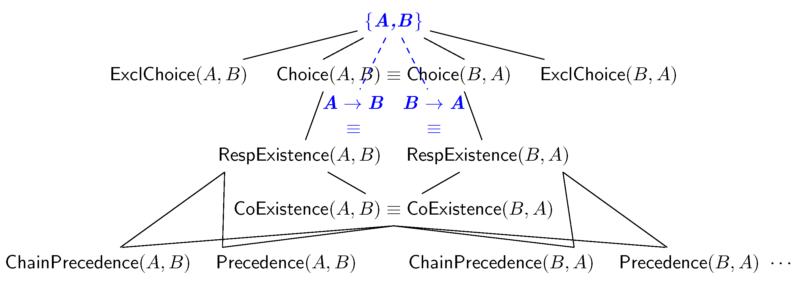
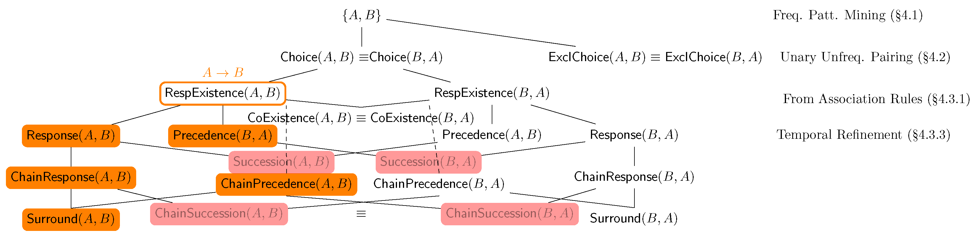
The implication notion can also be extended to declarative clauses in terms of their associated LTL_f semantics;  Figure 2 represents the entailment lattice of such declarative clauses, expressed as a Hasse diagram [32], and depicting the relationship among such clauses under the assumption of non-zero confidence (Section 6.1).

If a Declare specification contains one clause that predicates over event payloads as an activation/target/correlation condition, we refer to this as data-aware specification; otherwise, we refer to this as dataless. We state that the log is dataless if each event has an empty payload, otherwise, it is data-aware. For data-aware specifications, we can identify correlation conditions denoting disjunction conditions across target/activation conditions, as well as correlations between them. In this paper, we only consider dataless specifications and logs; thus, we omit the true data predicates associated with the activation/target conditions and only provide the activity labels. Therefore, throughout the rest of the paper, we denote each event ${\sigma }_j^i$ by only its associated activity label, A when all activity labels are considered as one character, we might represent each trace as a string of activity labels.

Example 1.

Our current logs of interest are dataless; thus, having events that contain empty payload functions ∅, we use ${\sigma }^i=$ ABC as the shorthand for ${\sigma }^i=\langle$ A,∅ 〉 〈 B,∅ 〉 〈 C, ∅〉.

Declarative clauses, therefore, involve the instantiation of declarative templates with activation and target conditions; by restricting our consideration to dataless specifications, such conditions restrict the possible activity label events by the one expressed by the activation (and target) conditions $\mathtt{A}$ (and $\mathtt{B}$). For example, $\mathsf{Precedence}(\mathtt{A},\mathtt{B})$ has A as an activation condition, as an occurrence of the first A requires checking whether no preceding B shall occur. We denote $\mathsf{ActLeaves}\left(c\right)$ as the set of traces containing at least one event satisfying an activation condition in c [2]. The clause activation might require the investigation of a possible target condition, where temporal occurrence is regulated by the template semantics. To demonstrate this, consider the following example: while $\mathsf{Response}(\mathtt{A},\mathtt{B})$ requires that the target conditions always follow the activations, $\mathsf{RespExistence}(\mathtt{A},\mathtt{B})$ only requires its existence across the trace, and holds no temporal constraints as the former. Some of the clauses listed in  Table 1 entail others, due to the stricter variation in the “temporal strictness” or the composition of multiple clauses. The previous example focuses on stricter temporal variation, while $\mathsf{CoExistence}(\mathtt{A},\mathtt{B})$ entails both $\mathsf{RespExistence}(\mathtt{A},\mathtt{B})$ and $\mathsf{RespExistence}(\mathtt{B},\mathtt{A})$.

We state that a trace ${\sigma }^i$ vacuously satisfies a Declare clause c if the trace satisfies such a clause without providing an event that satisfies the clause’s activation condition (i.e., ${\sigma }^i\vDash \left[\left[c\right]\right]\wedge {\sigma }^i\notin \mathsf{ActLeaves}\left(c\right)$). We can similarly frame the concept of vacuous violation. It occurs when a trace fails to satisfy a declarative clause, represented as (${\sigma }^i⊭\left[\left[c\right]\right]\wedge {\sigma }^i\notin \mathsf{ActLeaves}\left(c\right)$).

Declare walks in the footsteps of association rule mining by providing definitions of confidence and support metrics associated with declarative clauses. Still, the current literature provides disparate definitions of those metrics, depending on the specific context of interest [2,20], exploiting different clause “applicability” notions. Our previous work [2] considers “applicability” in terms of mere clause satisfiability, thus considering traces either vacuously or non-vacuously, satisfying a given declarative clause, while straightforwardly considering the traces containing the activation conditions as the denominator for the confidence score:

$${\mathrm{S}\mathrm{UPP}}_{\mathfrak{S}}\left(c\right)=\frac{\left|\{{\sigma }^i\in \mathfrak{S}\mid {\sigma }^i\vDash \left[\left[c\right]\right]\}\right|}{\left|\mathfrak{S}\right|}{\mathrm{C}\mathrm{ONF}}_{\mathfrak{S}}\left(c\right)=\frac{\left|\{{\sigma }^i\in \mathfrak{S}\mid {\sigma }^i\vDash \left[\left[c\right]\right]\}\right|}{\left|\mathsf{ActLeaves}\right(c\left)\right|}$$

(4)

As the notion of Supp is directly related to the satisfiability of a given declarative clause, despite its inclusion of the vacuously satisfied traces, this makes it the ideal candidate for the basis of an anti-monotonic quality criterion (Lemma A4) for implementing the lattice search within a general-to-specific heuristic algorithm for the hypothesis search. Still, this definition of confidence is not normalised between zero and one, as the number of traces potentially satisfying the clause are much larger than the ones satisfying and providing an activation condition to the clause.

By restricting the notion of “applicability” to the sole traces containing activation conditions, we can have the notion of restrictive support and confidence [20], ensuring that the clause will fully represent the data if the evidence for both activation and (possibly) target conditions are given:

$$\mathrm{RS}\mathrm{U}\mathrm{P}{\mathrm{P}}_{\mathfrak{S}}\left(c\right)=\frac{\left|\{{\sigma }^i\in \mathfrak{S}\cap \mathsf{ActLeaves}\left(c\right)\mid {\sigma }^i\vDash \left[\left[c\right]\right]\}\right|}{\left|\mathfrak{S}\right|}$$

(5)

$$\mathrm{RC}\mathrm{O}\mathrm{N}{\mathrm{F}}_{\mathfrak{S}}\left(c\right)=\frac{\left|\{{\sigma }^i\in \mathfrak{S}\cap \mathsf{ActLeaves}\left(c\right)\mid {\sigma }^i\vDash \left[\left[c\right]\right]\}\right|}{\left|\mathsf{ActLeaves}\right(c\left)\right|}$$

(6)

Still, these two definitions each come with an intrinsic limitation. First, we can easily observe that RSupp is not anti-monotonic in the same way as Supp and, therefore, cannot be chosen as a quality criterion candidate for traversing the declarative hypothesis space (Section 6.2). Second, the authors showcasing ${\mathrm{RC}\mathrm{ONF}}_{\mathfrak{S}}$ assumed that, for Precedence(A,B), B should have been an activation condition, while this should have never really been the case, as the clause only postulates that B shall not appear before the first A, but nothing is stated on whether Bs shall occur after an occurrence of A. For this particular clause, there is a requirement for a redefined declarative confidence that ranges between 0 and 1. This new definition aims to provide a more restrictive understanding of confidence, especially in the presence of arbitrary activations or vacuous conditions within the trace. These force us to propose a novel specification of this restrictive confidence, which is a topic we will delve into in Section 3.1.

KnoBAB [2] is a columnar-based relational database, built with the prime purpose of optimizing formal verification for temporal data represented as event logs. This was achieved through the provision of relational semantics to the LTL_f operators, namely xtLTL_f, while providing a one-to-one mapping between the provided temporal operators and the LTL_f logical operators. The encoding of specific temporal operators for the relational model was mainly due to the inadequacy of the relational query plans and physical operators to efficiently compute such tasks over customary relational models [30]. The definition of xtLTL_f operators facilitates the expression of formal verification tasks as relational database queries. These queries not only return the trace that satisfies the specification but also provide details on the events that activate, target, and correlate with one another. xtLTL_f also allows the identification of query plan optimisation strategies. First, we minimise access to the data tables by fusing entire sub-expressions, providing the same temporal behaviour, including the query plan leaf nodes that directly access the temporal information stored as relational tables. Second, we can further pre-process this query plan to achieve trivial intra-query parallelism. As the aforementioned query plan transformation converts an abstract syntax tree into a direct acyclic graph, we can now run a topological sort algorithm to determine the operators’ order of execution after representing them as nodes within the query plan. This allows the additional transformation of the aforementioned direct acyclic graph into a dependency graph, represented as a layered graph. As each node belonging to a given layer shares no computational dependencies with the other, we can also define a scheduling order for the xtLTL_f operators, where the execution can be trivially parallelised, achieving straightforward intra-query parallelism. Third, we guarantee efficient data access through the provision of indexed relational tables containing temporal, payload, and event-counting information. The results provided in our previous research [2] show that the system achieves significant performance gains against state-of-the-art dataless and data-aware temporal formal verification systems, either ad hoc solutions or competing relational representations and queries expressing formal verification tasks directly in SQL.

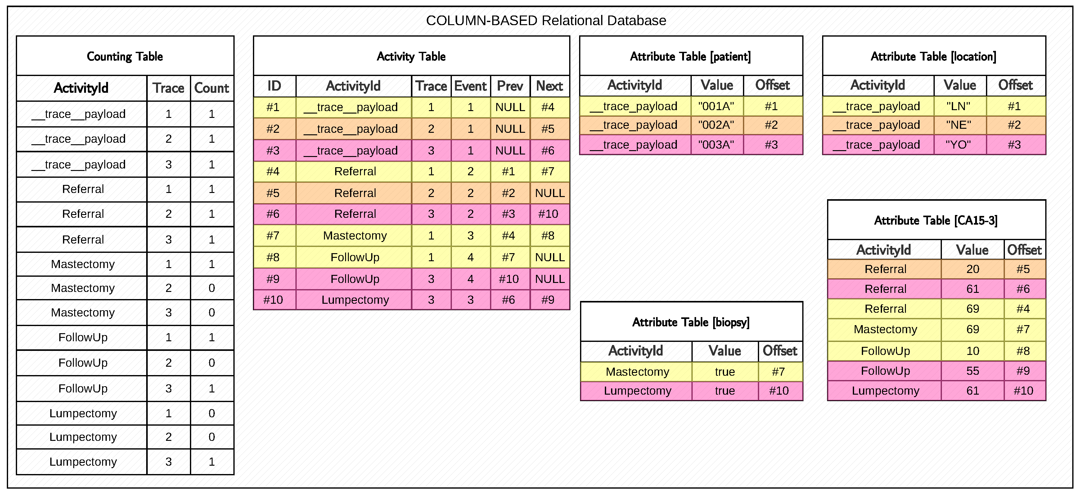
We will now describe in greater detail the relational table being exploited to store the log traces’ temporal behaviour, as both Bolt and the current algorithm leverage such architecture. Temporal data are loaded and processed into three types of tables depicted in Figure 3: ${\mathsf{CountingTable}}_{\mathfrak{S}}$, ${\mathsf{ActivityTable}}_{\mathfrak{S}}$, and ${\mathsf{AttributeTable}}_{\mathfrak{S}}$(s).

The ${\mathsf{CountingTable}}_{\mathfrak{S}}$ compactly stores the number of occurrences ${\#}_{{\sigma }^i}\mathtt{A}$ (count cell) for each activity label A (activityId cell) occurring in a trace ${\sigma }^i$ (trace cell) as a 64-bit unsigned integer, which is also used to sort the tables in ascending order. We also show the absence of events associated with a given activity label by setting the count field for a specific trace to zero. The space complexity associated with this table is $\Theta \left(\right|\Sigma |·|\mathfrak{S}\left|\right)$, while the occurrence count of a given activity for a specific trace can be retrieved in the $O\left(1\right)$ time complexity. This table facilitates the efficient computation of dataless ‘exists’ and ‘absence’ Declare clauses.

Example 2.

With reference to Figure 3 showcasing a KnoBAB relational representation for a healthcare log, determining whether a mastectomy event occurred at least once in ${\sigma }_1$ boils down to checking whether ${\#}_{{\sigma }^1}\mathit{Mastectomy}\ge 1$. As ${\#}_{{\sigma }^1}\mathit{Mastectomy}=1$, the aforementioned trace satisfies the desired condition.

As this table lacks any temporal information, we need to introduce a novel table that preserves this. Each row $\langle \mathtt{A},j,i,q,q^{\prime }\rangle$ in an ${\mathsf{ActivityTable}}_{\mathfrak{S}}$ states that the i-th event of the j-th trace (${\sigma }_i^j=\langle \mathtt{A},\delta \rangle$) is labelled as $\mathtt{A}$, while q (or $q^{\prime }$) is the pointer to the immediately preceding ${\sigma }_{i-1}^j$ (or following, ${\sigma }_{i+1}^j$) event within the trace, if any. NULLs from  Figure 3 in ${\mathsf{ActivityTable}}_{\mathfrak{S}}$  highlight the start (finish) event of each trace, where there is no possible reference to past (future) events. The primary index of the ${\mathsf{ActivityTable}}_{\mathfrak{S}}$  efficiently points to the first and last record associated with a given activity label in the $O\left(1\right)$ time complexity. As the table’s records are sorted by the activity label, trace ID, and event ID by storing them as 64-bit integers, we can retrieve all records containing a given activity across the log. Pointers provide efficient access to the events immediately preceding and following a given event without additional access to the table and a subsequent join across accessed data.

Example 3.

ChainPrecedence(FollowUp,Mastectomy) in our running example requires accessing all the activation conditions through the primary index of such a table, thus obtaining ${\mathit{ActivityTable}}_{\mathfrak{S}}.$ $primary\_index\left(\mathit{FollowUp}\right)=\langle \#8,\#9\rangle$. Now, we can iterate the table’s records, starting from no. 8 until no. 9 included. By exploiting the q Prev  pointers, we can determine that no. 8 has a preceding mastectomy  event while no. 9, also belonging to a different trace, has a preceding lumpectomy  event, thus violating the aforementioned clause. This leads to the main optimisation of mining ChainPrecedence and ChainSuccession clauses This assumption will be used implicitly in the code for mining such clauses in Section 4.3.3.

The secondary index of the ${\mathrm{ActivityTable}}_{\mathfrak{S}}$ maps each trace the ID to the first and last events. This is especially beneficial for declarative mining as we can directly return the first and last events of each trace, and are able to quickly mine Init/End clauses.

Example 4.

With reference to our running example, determining whether End(FollowUp) requires accessing the last event for all traces, as we obtain ${\mathit{ActivityTable}}_{\mathfrak{S}}.$ $secondary\_index\left({\sigma }^1\right)=\langle \#1,\#8\rangle$, ${\mathit{ActivityTable}}_{\mathfrak{S}}.$ $secondary\_index\left({\sigma }^2\right)=\langle \#2,\#5\rangle$, and ${\mathit{ActivityTable}}_{\mathfrak{S}}.$ $secondary\_index$ $\left({\sigma }^3\right)=\langle \#3,\#9\rangle$, only the first and the last events are associated with a FollowUp  event, while the second is a Referral. This leads to the main optimisation associated with Algorithm 5 for mining Init/Ends clauses.

${\mathrm{AttributeTable}}_{\mathfrak{S}}$-s guarantee faithfully reconstructing the entire log information by associating the payload information for each event in the activity table. In particular, we generate one table per key in the data payload. As our current algorithm does not rely on payload information $\delta$ stored in this table, we refer to [2] for further information.

2.3.2. Temporal Specification Mining

In traditional machine learning (Section 2.1), data provide the common specifications from which specifications are extracted. Data points ${\mathbf{x}}_i$ are usually associated with a classification label $y_i$, directly associating the data to the expected class of specifications. This is very different from customary formal methods, where a formula defines the correct expected behaviours over all possible inputs. When we are only interested in distinguishing between behaviour that adheres to a formal specification and that which does not, it is adequate to identify two distinct classes: one for traces conforming to the expected temporal property, and another for those that deviate from it [21]. Still, doing so when data are biased, limited, or labelled from non-experts might be challenging [1]. Specification mining attempts to bridge the gap between specifications and data by inferring the former from the latter.

In business process mining literature, specification mining is often referred to as declarative process (or model) mining. As in specification mining, we are interested in extracting specifications, where the language for the specification is expressed as a Declare clause. Apriori declarative mining (ADM) [20] represents an advancement in state-of-the-art declarative temporal specification mining algorithms [33] by limiting the instantiation of all possible declarative clauses to the itemsets being returned by an Apriori algorithm; such clauses are then further pruned through declarative minimum support thresholds, while prior solutions [33] instantiated every Declare clause with all conceivable templates, leading to a quadratic combination set. This constraint is also evident in the available implementation of Apriori declarative mining + Fisher score (ADM+S) in Python [21], where the actual implementation instantiates all the templates for all the possible activity labels being available on the current data. In fact, both [33] and [21] become easily intractable in real-world logs describing thousands of activities/events. ADM also further creams off infrequent declarative clauses through confidence and support. Notwithstanding the aforementioned improvements for candidate clause pruning, such approaches exploit no efficient heuristics for mining clauses. By only exploiting frequent itemset mining algorithms with support filtering for generating and testing all possible declarative clauses on log traces, the authors achieve suboptimal algorithms that generate and test all the candidate clauses (propositionalisation [23]), which are further creamed off through an additional filtering step.

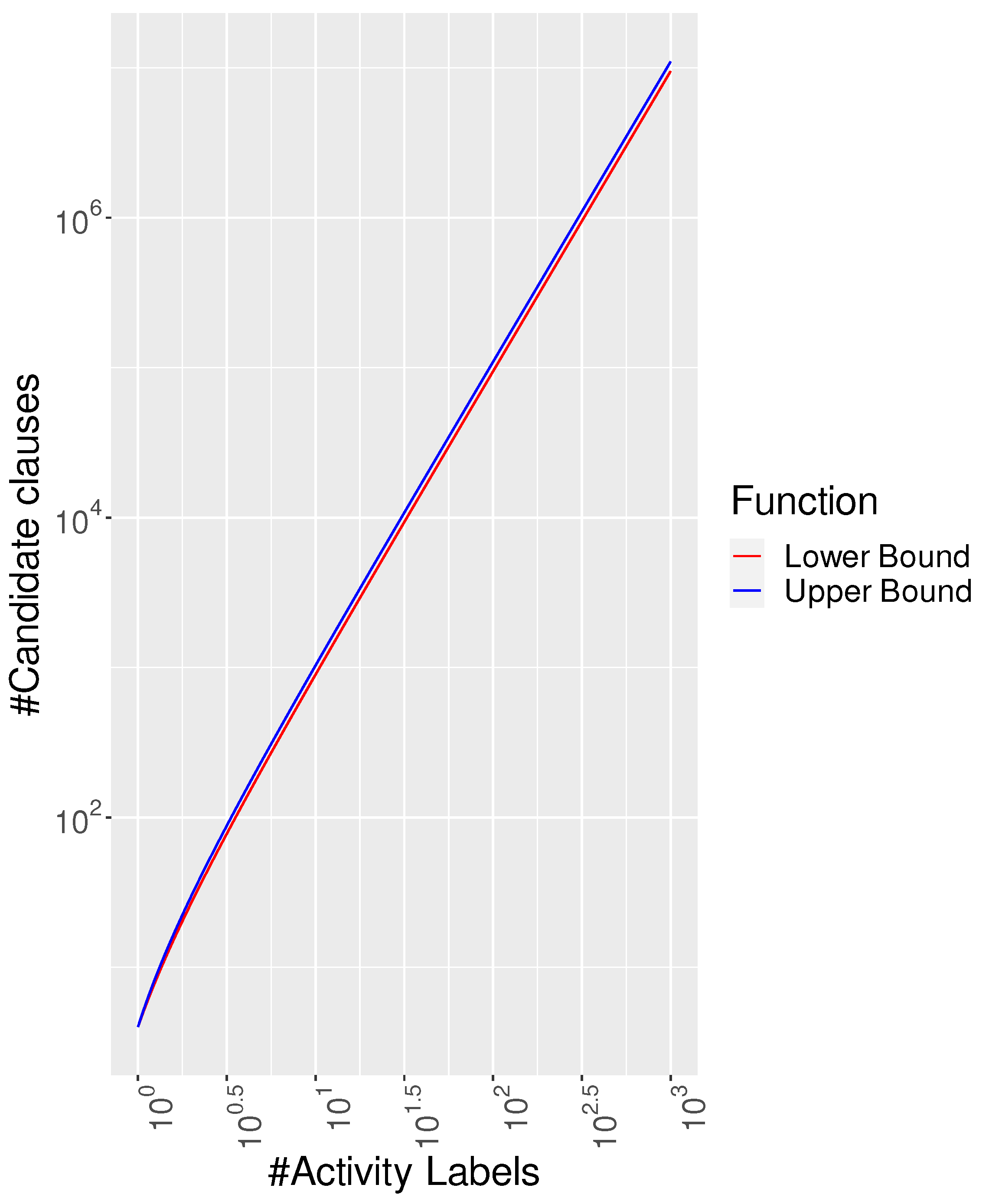
 Figure 4 provides a clear picture concerning the impossibility of generating, testing, and returning all possible clauses for realistic datasets containing many distinct events through exhaustive search and propositionalisation within a reasonable amount of time. As an upper bound to the total number of possible clauses to be returned, we can consider instantiating all possible pairs of activity labels for the 11 binary clauses and instantiating the 4 unary clauses with $n=0$ (Absence) or $n=1$ (Exists), thus obtaining the following:

$$UB\left(I\right)=11·\left(\right|I{|}^2-\left|I\right|)+4|I|$$

(7)

For the lower bound, we can limit the number of clauses for the 3 symmetric clauses of Choice, ExclChoice, and CoExistence to $\raisebox{1ex}{$\left|I\right|\left(\right|I|-1)$}\!\left/ \!\raisebox{-1ex}{$2$}\right.$ combinations, thus obtaining $LB\left(I\right)=\frac{1}{2}{\left(19\right|I|}^2-11\left|I\right|)$. We can easily see that, for hundreds of activity labels, as in realistic cybersecurity datasets, naïve algorithms are required to test an order of one million clauses, which cannot be analysed in a feasible amount of time. This clearly postulates the need for an efficient search algorithm limiting the search to the clauses effectively being representative of the data of interest.

Our previous implementation of dataless declarative process mining, i.e., Bolt [5], was designed to efficiently mine the twelve clauses listed in  Table 1; however, it excluded the two newly introduced clauses, Succession and ChainSuccession, and our novel proposal introduced in the present paper, Surround (Section 3.2). 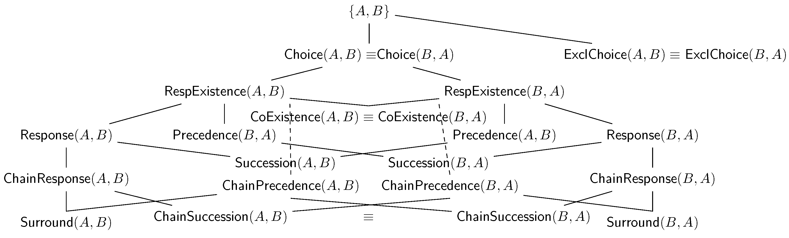Bolt outperforms all state-of-the-art dataless declarative mining competitors by leveraging KnoBAB’s aforementioned indexed tables while avoiding costly formal verification computations by only detecting vacuity and violation conditions without the need for combining multiple xtLTL_f operators, as they can generate considerable overhead due to the intermediate results being generated by the implementation of the relational operators. Moreover, declarative clauses are generated using a general-to-specific search, starting from frequent clauses being directly inferable from association rule mining, such as RespExistence and CoExistence, temporally refining them by starting the visit of the lattice in  Figure 5. To avoid generating uninteresting atemporal behaviour when temporal behaviour might be identified, we generate Choice and ExclChoice clauses by combining unary infrequent patterns. Our current solution further improves this by discarding the return of such clauses if any more informative temporal behaviour is returned (Section 4.3.5).

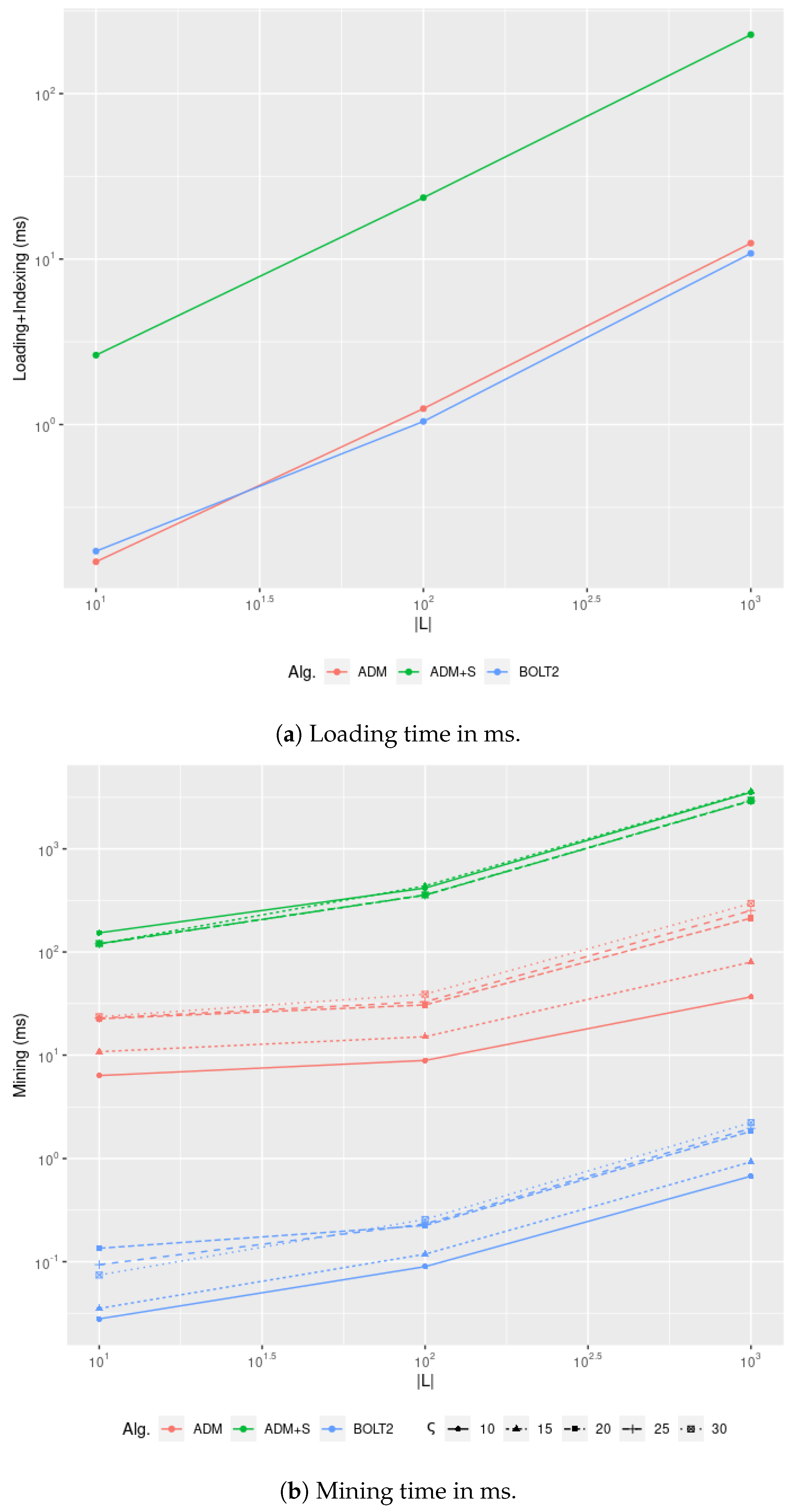
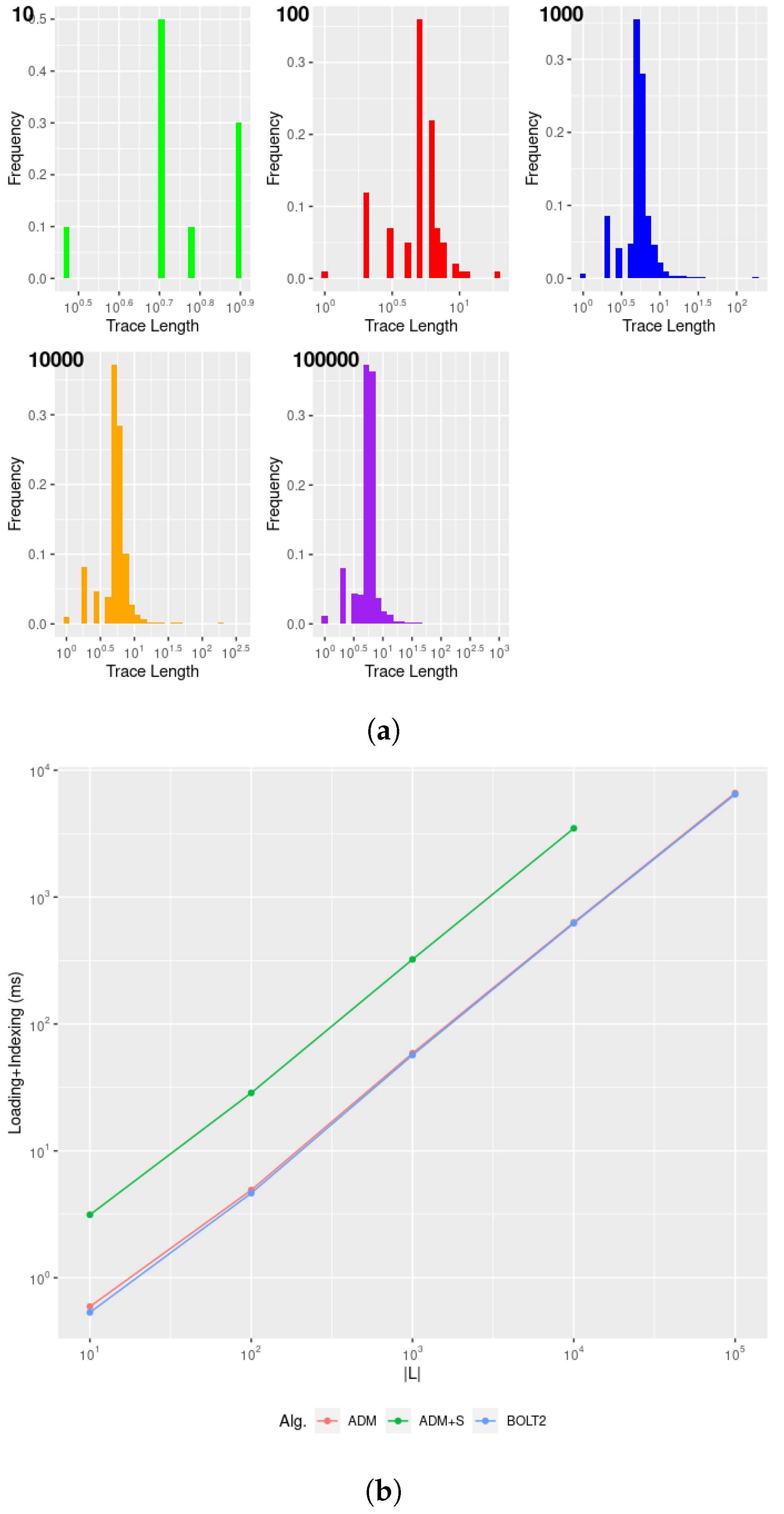
In our previous contribution, we compared our proposed algorithm to [5] TopN Declare  [30] using KnoBAB’s formal verification pipeline, Apriori declarative mining (ADM) after re-implementation on top of KnoBAB [20], and Apriori declarative mining + Fisher score (ADM+S) implemented in Python [21]. Through experiments, we demonstrated that we were both scalable with regard to the trace length and log size, while consistently outperforming the running time for all former competitors. TopN Declare was poor at mining all expected clauses from a log, as just considering all possible pairs among frequently occurring activity labels does not guarantee returning all the relevant clauses, and the others suffered greatly by producing explosive and redundant specifications, achieving hundreds of clauses, even with a strict support threshold $\theta$, as these solutions are affected by the curse of propositionalisation required to instantiate and test all possible clauses that might be generated from some mined binary frequent patterns. Bolt avoids the computational overhead from prior approaches due to the reduction of the specification mining task to a conformance checking one and its associated data allocation footprint by directly scanning relational tables without the need for generating intermediate results, as enforced by the adoption of query operators. Different from previous mining approaches that required instantiating all possible declarative clauses over all possible frequent itemsets through extensive clause propositionalisation, Bolt exploits a preliminary branch-and-bound solution for pruning irrelevant or “redundant” clauses, avoiding testing to abide by some irrelevant clauses that are not represented within the data (Example 13). The frequent support and confidence of itemsets serve as heuristics for determining whether specific clauses are frequent or appear in the specification, thus narrowing down the testing of temporal patterns to only the relevant instances.

Despite Bolt outperforming state-of-the-art temporal specification mining algorithms while mining less superfluous and more descriptive specifications, this approach can still be significantly improved. First, despite Bolt being able to prune many redundant clauses that do not aptly describe the log compared to other solutions, the outputted specification is still far from minimised, as there still exist redundant clauses that imply each other. Improving this requires avoiding returning Choice clauses for temporal declarative clauses that have already been considered if appearing with greater or equal support. Second, this preliminary solution still returns multiple symmetric clauses, which are deemed as equivalent, e.g., $\mathsf{CoExistence}(\mathtt{A},\mathtt{B})$ is completely equivalent to $\mathsf{CoExistence}(\mathtt{B},\mathtt{A})$, as they refer to the same set of log traces. Third, we still return multiple clauses entailing each other, not fully exploiting the lattice descent for ensuring specification size minimality via the computation of an S-border. Any desired improvement of Bolt tackling all these limitations with minimal performance costs will provide specifications returning more specific clauses while being less verbose than Bolt, while outperforming all other competitors by at least one order of magnitude. Our methodology section (Section 4) shows how our novel solution addresses all such limitations.

3. Theoretical Contributions

This section provides preliminary theoretical definitions that are needed before introducing our improved algorithm discussed in the methodology section (Section 4). After enhancing the restrictive definition of confidence (Section 3.1), we describe our newly proposed clause, Surround (Section 3.2), where we envision pruning heuristics jointly with ChainSuccession to avoid costly violation checks (Section 3.3). Finally, we discuss a notion of generality and quality criteria for shaping the S-border to ensure specification minimality (Section 3.4).

Table 2. Table of notation for symbols $\chi \in \mathcal{T}$ defined as ($\chi :=\mathcal{E}$) or characterised by ($\mathcal{E}\left(\chi \right)$) $\mathcal{E}$.

Symbol ($\mathit{\chi }$)	Definition ($\mathcal{E}$)	Type ($\mathcal{T}$)	Comments
Set Theory for Data Mining
∅		Set	An empty set contains no items.
$(⪯,S)$			A partially ordered set (poset) is a relational structure for which ⪯ is a partial ordering over S [32]. ⪯ over S might be represented as a lattice, referred to as the Hasse diagram.
$\complement C$	$\mathcal{U}\setminus C$	Set	Complement set: given a universe $\mathcal{U}$, the complement returns all of the elements that do not belong to C.
$\left|C\right|$	${\sum }_{c\in C}1$	$\mathbb{N}$	The cardinality of a finite set indicates the number of contained items.
$\wp \left(C\right)$	$\left\{T\right|T\subseteq C\}$	Set	The power set of C is the set whose elements are all of the subsets of C.
$Y^X$	$\left\{f\right|f:X\to Y\}$	Set	Set exponentiation.
${\mathbf{1}}_B\left(x\right)$	$\left\{\begin{array}{cc}1\hfill & B\left(x\right)\hfill \\ 0\hfill & \mathrm{oth}.\hfill \end{array}\right.$	$D\to \{0,1\}$	Indicator function.
${⪯}^b$	Def. 2	Relationship	Bolt2 generality relationship.
${\mathcal{Q}}^b$	Def. 3	Predicate	Bolt2 quality criterion.
Frequent Patterns and Association Rules
I		Set	Finite set of occurring atoms, also providing a finite set of activity labels.
i		$\wp \left(I\right)$	A possible itemset (i), or a transaction (t).
T		Set	The set of all possible transactions.
${\varsigma }^{\prime }\left(i\right)$	Equation (1)		Itemset support for i with respect to some transactions T.
$\varsigma \left(i\right)$	$\raisebox{1ex}{${\varsigma }^{\prime }\left(i\right)$}\!\left/ \!\raisebox{-1ex}{$\left|T\right|$}\right.$		Normalised itemset support for i w.r.t some transactions T.
$\mathtt{T}\to \mathtt{H}$		Rule	Binary association rule composed of a tail T and a head H.
$\mathtt{s}(\mathtt{T}\to \mathtt{H})$	Equation (2)		Support for association rule $\mathtt{T}\to \mathtt{H}$.
$\mathtt{c}(\mathtt{T}\to \mathtt{H})$	Equation (2)		Confidence for association rule $\mathtt{T}\to \mathtt{H}$.
LTLf & Declare
${\sigma }_j^i$	$\langle {\mathtt{A}}_j,{\delta }_j\rangle \simeq {\mathtt{A}}_j$	$\mathsf{\Sigma }\times V^K$	Event
${\sigma }^i$	${\sigma }_1^i,\dots ,{\sigma }_n^i$	Sequence	Trace, sequence of temporarily ordered events.
$\mathfrak{S}$	$\{{\sigma }^1,\dots ,{\sigma }^m\}$	Set of traces	System or Log.
⊧			$\mathfrak{S}\vDash \mathsf{\Phi }$ denotes that $\mathsf{\Phi }$ is satisfied for the world/system $\mathfrak{S}$.
Supp${}_{\mathfrak{S}}\left(c\right)$, RSupp${}_{\mathfrak{S}}\left(c\right)$	Equations (4) and (5)		(Restrictive) support for a declarative clause c over a log $\mathfrak{S}$.
Conf${}_{\mathfrak{S}}\left(c\right)$, RConf${}_{\mathfrak{S}}\left(c\right)$	Equations (4) and (6)		(Restrictive) confidence for a declarative clause c over a log $\mathfrak{S}$.
RConf${}_{\mathfrak{S}}^{+}\left(c\right)$	Equation (8)		Enhanced restrictive confidence for a clause c over a log $\mathfrak{S}$.
Pseudocode
↑			Null pointer or terminated iterator.
Next$\left(\mathit{it}\right)$		Pointer	On $\mathit{it}$ non-null, it increments the pointer it to the next element in the stream/sequence
Current$\left(\mathit{it}\right)$		Dereference	Element pointed by the pointer/iterator it.
${\mathit{act}}_{\mathtt{A},\mathtt{B}}^{★}$	$\mathsf{ActLeaves}\left({★}_{\mathtt{A},\mathtt{B}}\right)$	Set	Set of activated traces for the clause $★(\mathtt{A},\mathtt{B})$.
${\mathit{viol}}_{\mathtt{A},\mathtt{B}}^{★}$		Set	Set of traces violating clause $★(\mathtt{A},\mathtt{B})$.
${\mathit{sat}}_{\mathtt{A},\mathtt{B}}^{★}$	$\complement {\mathit{viol}}_{\mathtt{A},\mathtt{B}}^{★}$	Set	Set of traces satisfying clause $★(\mathtt{A},\mathtt{B})$.
${\mathit{vac}}_{\mathtt{A},\mathtt{B}}^{★}$		Set	Set of traces containing no event being activated by A for $★(\mathtt{A},\mathtt{B})$.

summarises the notation used throughout the paper.

3.1. Enhanced Restrictive Confidence

During our extension of the declarative metrics, we found that the definition of restrictive confidence in Section 2.3.1 did not encompass all the possible formulations of activations and targets in Declare clauses. This is mainly due to the semantics of Precedence(A,B), as well as the “correct” interpretation of what an activation for such a clause should be. Here, $\mathtt{A}$ is our activation, as in LTL_f, we need to scan the first $\mathtt{A}$s of each trace and check for $\neg \mathtt{B}$ in the past. Precedence is distinct from the other declarative clauses as the lack of activation does not guarantee vacuous satisfiability because it can be violated without any activation at all via $\square (\neg \mathtt{B})$. By considering this, we obtain our upgraded metric by considering the cases where the trace was either activated or vacuously violated.

Definition 1.

Enhanced restrictive confidence expresses the ratio between traces in $\mathfrak{S}$ both satisfying and activating a declarative clause c of the overall number of traces, either activating the declarative clause (without necessarily satisfying it) or not satisfying the clause at all.

$${\mathrm{RC}\mathrm{ONF}}_{\mathfrak{S}}^{+}\left(c\right)=\frac{\left|\{{\sigma }_i\in \mathfrak{S}\cap \mathit{ActLeaves}\left(c\right)\mid {\sigma }_i\vDash \left[\left[c\right]\right]\}\right|}{|\mathit{ActLeaves}\left(c\right)\cup \{{\sigma }_i\in \mathfrak{S}|{\sigma }_i⊭\left[\left[c\right]\right]\}|}$$

(8)

Example 5.

Consider the log $\mathfrak{S}=\left\{{\sigma }^1,{\sigma }^2,{\sigma }^3\right\}$ with traces ${\sigma }^1=$ ABB, ${\sigma }^2=$ CAA, and ${\sigma }^3=$ CCB. Let c be a clause Precedence(A,B). ${\sigma }^1$ is activated and satisfied with both activation and target conditions, and ${\sigma }^2$ is satisfied, containing an activation only. However, ${\sigma }^3$ provides a case that is not considered by the other clauses; we have no activation, A, but the clause is still violated. We consider ${\sigma }^3$ as vacuously violating c as it violates $\square (\neg \mathit{B})$, while the others are non-vacuously satisfied. For Precedence, we have RConf${}_{\mathfrak{S}}\left(c\right)=1.0$. However, this does not consider the vacuous violation from trace ${\sigma }^3$.

By using the novel formulation above, we obtain the expected RConf${}_{\mathfrak{S}}^{+}\left(c\right)=\frac{2}{3}$.

3.2. Surround

We propose a novel Declare clause, Surround, providing a unique temporal behaviour. We might argue that Surround is not required due to the existence of ChainSuccession, as they both describe similar temporal behaviours. Still, the latter does not prescribe that an event might be both preceded and followed by a given one as the former. $\mathsf{Surround}$ describes the following unique temporal constraint: every activation is immediately preceded by and immediately followed by the target. In the context of data-aware specifications and logs, we can exploit this clause to express the idea that the occurrence of an activation event should not affect the post-conditions of the event that should then match the pre-conditions, thus adequately describing invariant behaviour.

Example 6.

Consider the following log:

$$\mathfrak{S}=\left\{{\sigma }^1,{\sigma }^2,{\sigma }^3\right\}{\sigma }^1=\mathit{CBAB},{\sigma }^2=\mathit{BBD},{\sigma }^3=\mathit{CCBAB}$$

We have that ChainSuccession(A,B) has zero support as all the traces violate the constraint, while Surround(A,B) has a perfect support. In fact, the latter is defined as $\mathit{ChainResponse}(\mathit{A},\mathit{B})\wedge \mathit{ChainPrecedence}(\mathit{A},\mathit{B})$, while the former is defined as $\mathit{ChainResponse}(\mathit{A},\mathit{B})\wedge \mathit{ChainPrecedence}(\mathit{B},\mathit{A})$.

We can formally prove that $\mathsf{ChainSuccession}(\mathtt{A},\mathtt{B})\ne \mathsf{Surround}(\mathtt{A},\mathtt{B})$ by showing that there exists at least one trace differentiating the behaviours of the two clauses (Lemma A5).

3.3. Pruning Heuristics

The following pruning heuristics aim to avoid computing costly trace scanning and testing for specific temporal patterns if we can efficiently test a numerical condition that encompasses the violation of a clause by a substantial number of traces within the log. Formulating such heuristics as conditions to be checked on the ${\mathsf{ActivityTable}}_{\mathfrak{S}}$  will not be deemed as adequately efficient as it would require extra scans that will still boil down to the punctual detection of dissatisfying traces, we aim to determine early stopping conditions on the ${\mathsf{CountingTable}}_{\mathfrak{S}}$  when applicable. We identify two heuristics, one for $\mathsf{ChainSuccession}$ and the other for $\mathsf{Surround}$.

We now discuss the novel improved heuristics, replacing the ones from our previous paper. Any trace satisfying $\mathsf{ChainSuccession}(\mathtt{A},\mathtt{B})$ should have the same number of As as B. However, we also need to consider that B might also occur at the beginning of a trace, for which no $\mathsf{ChainPrecedence}(\mathtt{B},\mathtt{A})$ is activated. This provides a new bound for the number of As within a trace, which should be one less than the number of Bs. This leads to the following lemma:

Lemma 1.

A trace ${\sigma }^i$ violates not-vacuously $\mathit{ChainSuccession}(\mathit{A},\mathit{B})$ upon violation of the following constraint: ${\#}_{{\sigma }^i}\mathit{B}-{\mathbf{1}}_{{\sigma }_1^i=\langle \mathit{B},{\delta }^i\rangle }\le {\#}_{{\sigma }^i}\mathit{A}\le {\#}_{{\sigma }^i}\mathit{B}$.

Consider that ${\mathbf{1}}_P$ is the indicator function returning 1 upon verification of the predicate P, and 0 otherwise. We can infer a similar constraint for $\mathsf{Surround}(\mathtt{B},\mathtt{A})$ in the worst-case scenario, where activation never occurs at the start of a trace, events labelled as B must occur both before and after event A. Conversely, in the best-case scenario, when A occurs at the start of the trace, there is no need for a preceding B event before such A:

Lemma 2.

A trace ${\sigma }^i$ violates non-vacuously $\mathit{Surround}(\mathit{A},\mathit{B})$ upon violation of the following constraint: ${\#}_{{\sigma }^i}\mathit{A}\le {\#}_{{\sigma }^i}\mathit{B}\le 2·{\#}_{{\sigma }^i}\mathit{A}$.

Correctness proofs for both lemmas are presented in Appendix C.

3.4. Clause Generality and Quality Criterion for Mining

The generality relationship of choice for our mining algorithm formalises the notion implicitly provided in our previous paper [5]. This notion is required to guarantee the correctness of our mining algorithm and avoid returning evidence from the data due to vacuous satisfiability.

Definition 2

(Bolt2 Generality). Given a log $\mathfrak{S}$, we state that a declarative clause $c^{\prime }$ is more general than c (and we denote this as $c^{\prime }{⪯}^{b}c$) if c implies $c^{\prime }$, while both are activated by at least one trace in $\mathfrak{S}$:

$$c^{\prime }{⪯}^{b}c\iff c\Rightarrow c^{\prime }\wedge {\mathrm{RC}\mathrm{ONF}}_{\mathfrak{S}}^{+}\left(c\right)>0\wedge {\mathrm{RC}\mathrm{ONF}}_{\mathfrak{S}}^{+}\left(c^{\prime }\right)>0$$

Observe that this definition follows from the correlation between the coverage and clause implication (Lemma A3) while also guaranteeing the usage of the Supp metric as an anti-monotonic metric for general-to-specific algorithms for lattice descent (Lemma A4 and Corollary A1). Due to this, our algorithm is also going to exploit this metric as an early stopping condition, thus avoiding further refining clauses that might provide infrequent support from the data. Furthermore, generating preliminary clauses from non-zero confidence association rules guarantees the generation of refined clauses with non-zero enhanced restrictive support, while also guaranteeing the traversal of the lattice from the most specific hypothesis to a more general one (Section 6.2). This definition enables a specific definition for a refinement function $\rho$ using ${⪯}^b$ as a generality relation.

We then leverage the former definition of generality for specifying our quality criterion for our general-to-specific hypothesis (i.e., clause) search. Before saying so, we want to state that clause c is “stronger” (in our previous paper, this notion was referred to as “consumption”) than $c^{\prime }$ if (i) the coverage of the former is greater than the one of the latter, (ii) all the traces accepted by c are also accepted by $c^{\prime }$ (i.e., $c\Rightarrow c^{\prime }$), and (iii) its support is lower-bounded by a minimum support threshold $\theta$. The first property favours clauses covering most of the traces from the log while still satisfying the minimal quality criterion. Given this requirement, we provide a quality criterion for a clause c over a log $\mathfrak{S}$, dictating that c be stronger than any possible clause $c^{\prime }$ for which c is a refinement.

Definition 3

(Bolt2 quality criterion). A clause c satisfies the quality criterion over a log $\mathfrak{S}$ if this appears stronger than any clause for which it is a direct refinement.

$${\mathcal{Q}}^b(c,\mathfrak{S})\iff (\forall c^{\prime }.c\in \rho \left(c^{\prime }\right)\Rightarrow {\mathrm{S}\mathrm{UPP}}_{\mathfrak{S}}\left(c^{\prime }\right)\le {\mathrm{S}\mathrm{UPP}}_{\mathfrak{S}}\left(c\right))\wedge {\mathrm{S}\mathrm{UPP}}_{\mathfrak{S}}\left(c\right)\ge \theta \wedge {\mathrm{RC}\mathrm{ONF}}_{\mathfrak{S}}^{+}\left(c\right)>0$$

Observe that this quality criterion can also be further simplified after observing that Supp is anti-monotonic (Corollary A2).

Example 7.

By leveraging the same log from Example 6, $\mathrm{S}\mathrm{U}\mathrm{P}\mathrm{P}\left(\mathit{Response}(\mathit{D},\mathit{B})\right)=\frac{2}{3}$, as ${\sigma }^2$ contains no B events following D, and the remaining clauses are vacuously satisfied, while the support of $\mathit{RespExistence}(\mathit{D},\mathit{B})$ is $1.0$ as ${\sigma }^2$ contains a B event as well as a D. In our proposed approach, we advocate returning the latter instead of the former, as it provides better data coverage, thus minimising the risk of returning clauses overfitting the temporal behaviour of traces.

4. Methodology

Our proposed specification mining algorithm Bolt2 (Algorithm 3) can be seen as the repeated application of the general-to-specific hypothesis search (Algorithm 2) for each frequent pair of activity labels $\left\{\mathtt{A},\mathtt{B}\right\}$ frequently occurring in the log that generates binary declarative clauses (Algorithm 6 Line 6), while unary patterns are treated separately (Algorithm 5). We also extend the mining algorithm with pruning and inference heuristics, discarding costly tests of clauses not being representative of the log. This log then describes the data D of interest for the algorithm. At the same time, the hypothesis space ${\mathfrak{L}}_h$ for our declarative clause is derived from the instantiation of all possible templates from  Table 1 with both $\left\{\mathtt{A},\mathtt{B}\right\}$ and $\left\{\mathtt{B},\mathtt{A}\right\}$. The generality relation ${⪯}^b$, essential for the refinement operator $\rho$, as well as the quality criterion ${\mathcal{Q}}^b$, are defined in Section 3.4.

Algorithm 3 Bolt2

1: function Bolt2($\mathfrak{S},\theta$) 2:       $P\leftarrow$GenerateFrequentItemsets($\mathfrak{S},\theta$)                                ▹ Algorithm 4 3:       ChoiceFilter$,{\mathsf{\Phi }}^{\prime }\leftarrow$GenerateUnaryClauses(P)              ▹ Algorithm 5 4:       return ${\mathsf{\Phi }}^{\prime }\cup$BinaryClauseMining($P,\mathtt{ChoiceFilter},\theta$)             ▹ Algorithm 6

We now describe the specific implementation of such an algorithm. This accepts a log $\mathfrak{S}$ loaded and indexed as a knowledge base in KnoBAB, as well as a minimum support threshold $\theta$, and returns a list of declarative clauses to be considered as part of a conjunctive declarative specification $\mathsf{\Phi }$. As with our previous mining algorithm, Bolt  [5], we avoid mining clauses that are completely vacuously satisfied through association rule confidence. This is further enhanced by our notion of Supp while ensuring that at least one trace also activates the associated clause. This is extremely important for ensuring the correctness of our proposed lattice descent and ascent (Section 6.1).

We now motivate the adoption of this novel algorithm in light of the limitations of Bolt, as discussed in Section 2.3.2.

First, regarding Choice and ExclChoice, we generate such clauses by either pairing infrequent unary label with events having other activity labels or by returning a (Excl)Choice clause if no suitable temporal binary clause was not already returned. We also change the policy for returning Init and End clauses by returning them only if they satisfy the whole log.

Second, for symmetrical clauses $\mathsf{c}(\mathtt{A},{\mathtt{A}}^{\prime })\iff \mathsf{c}({\mathtt{A}}^{\prime },\mathtt{A})$, where both arguments are to be considered as activations, such as Choice, ExclChoice, and CoExistence, we also consistently prefer one of the two options by preferring the activity label appearing before the other one as the first argument of the clause.

Third, we further reduce the amount of returned clauses by discarding any Choice clauses if any other more refined clause is returned, as well as using the quality metric discussed in Section 3.4. To achieve this, we strictly abide by the entailment lattice described in  Figure 6. In particular, considering the non-zero support constraint, the general-to-specific traversal of the lattice exploits the refinement relationship $\rho$ using the associated generality relation ${⪯}^b$ from the previous section. Implementation-wise, this is achieved by always preferring the most refined clause at the same support conditions and avoiding returning the more general clauses if a clause with greater support is already returned.

The algorithm proceeds as follows: After generating the frequent itemsets with a maximum size 2 via FPGrowth (Section 4.1), we generate Exists/Absence clauses for certain unary patterns and prepare the generation of binary clauses by combining infrequent unary patterns or directly exploiting the mined binary patterns (Section 4.2). The last phase effectively generates such binary clauses through a preliminary heuristic phase via association rule mining, allowing further pruning of declarative clauses to be tested and considered (Section 4.3). Algorithm 3 shows the mutual dependencies of such tasks regarding input/output parameters.

4.1. Frequent Pattern Mining

In our first step described in Algorithm 4, we transform the temporal data stored in KnoBAB as transactions that are suitable for our implementation of the FPGrowth algorithm. This is rewritten from scratch due to errors in the previous library (https://github.com/integeruser/FP-growth, accessed on 10 August 2023) of choice, where bugs lead to inaccurate support ${\varsigma }^{\prime }$ computations, thus enforcing an estimate of the overall support through approximations. This phase now generates frequent itemsets suitable for the next association rule-mining phase.

Algorithm 4 Running FPGrowth over KnoBAB

1: function GenerateFrequentItemsets($\mathfrak{S},\theta$) 2:       $\varsigma \leftarrow {\left[\mathtt{A}\mapsto \left|\left\{{\sigma }^i|{\#}_{{\sigma }^i}j>0\right\}\right|\right]}_{\mathtt{A}\in I}$ 3:       $T\leftarrow {[i\in I|{\#}_{{\sigma }^j}i>0]}_{{\sigma }^j\in \mathfrak{S}}$ 4:       return FPGrowth($\varsigma$,T,$\theta$,$\mathcal{l}=2$)

As applying the FPGrowth algorithm over a log requires discarding the temporal information associated with a trace, as transactions merely list the occurrence of items/activity labels, we exploit our ${\mathsf{CountingTable}}_{\mathfrak{S}}$ as a transactional representation of our log. Any transaction $t_i$ associated with a temporal trace ${\sigma }^i$ will contain an item j if ${\sigma }^i$ has at least one occurrence of j, i.e., $j\in t_i\iff \left({\#}_{{\sigma }^i}j\right)>0$ (Line 3). Given this correspondence, we can then determine the item frequency table ${\varsigma }^{\prime }$ associated with our log as required by the FPGrowth algorithm by counting the traces containing at least one event with a given activity label A (Line 2). Such an algorithm can then be run with a minimum support threshold $\theta$, consistent with previous literature. As we are only interested in unary and binary clauses, we generate frequent itemsets that have a maximum length of $\mathcal{l}=2$ and support at least $\theta$. The algorithm then returns the frequently mined itemsets ${\pi }_i\in P$ with support ${\varsigma }^{\prime }\left({\pi }_i\right)$ (Line 4).

4.2. Unary Clause Mining and Binary Clauses Pre-Processing

The phase described in Algorithm 5 combines the infrequent unary itemsets in P for later generating Choice and ExclChoice clauses, while directly yielding unary declarative patterns for certain itemsets. The clauses being generated in this phase share the same certain ($100\%$) values for Supp, RSupp, and RConf${}^{+}$.

Algorithm 5 Generating unary clauses

1: function GenerateUnaryClauses(P) 2:       ChoiceFilter$\leftarrow \varnothing$; $\mathsf{\Phi }\leftarrow \varnothing$ 3:       for all $\langle {\pi }_i=\left\{\mathsf{A}\right\},\varsigma \left({\pi }_i\right)\rangle \in P$ do                                                           ▹Certain singlets 4:             if $\varsigma \left({\pi }_i\right)=100\%$ then 5:                  $n\leftarrow {arg\; min}_{{\sigma }^i}{\#}_{{\sigma }^i}\mathtt{A}>0$ 6:                  $N\leftarrow {arg\; max}_{{\sigma }^i}{\#}_{{\sigma }^i}\mathtt{A}>0$ 7:                  $\mathsf{\Phi }\leftarrow \mathsf{\Phi }\cup \{\langle \mathsf{Exists}(\mathsf{A},n),100\%\rangle ,\langle \mathsf{Absence}(\mathsf{A},N+1),100\%\rangle \}$ 8:             else 9:                  ChoiceFilter $\leftarrow \mathtt{ChoiceFilter}\cup \left\{\mathsf{A}\right\}$ 10:            end if 11:      end for 12:      Init$\leftarrow \left\{\right\}$; Ends$\leftarrow \left\{\right\}$ 13:      for all ${\sigma }^i\in \mathfrak{S}$ do 14:            ${\sigma }_1^i=\langle \mathtt{A},\delta \rangle$; ${\sigma }_{|{\sigma }^i|}^i=\langle \mathtt{B},\delta \rangle$        ▹ Retrieving this information through secondary index 15:            Init[A]← Init[A]+1 16:            Ends[B]← Ends[B]+1 17:      end for 18:      for all $\mathtt{A}\in I$ s.t. Init[A] $=\left|\mathfrak{S}\right|$ do 19:            $\mathsf{\Phi }\leftarrow \mathsf{\Phi }\cup \left\{\langle \mathsf{Init}\left(\mathtt{A}\right),100\%\rangle \right\}$ 20:      end for 21:      for all $\mathtt{B}\in I$ s.t. Ends[B] $=\left|\mathfrak{S}\right|$ do 22:            $\mathsf{\Phi }\leftarrow \mathsf{\Phi }\cup \left\{\langle \mathsf{End}\left(\mathtt{B}\right),100\%\rangle \right\}$ 23:      end for 24:      return ChoiceFilter, $\mathsf{\Phi }$

We now consider the unary frequent itemsets ${\pi }_i$ with support $\varsigma \left({\pi }_i\right)$ generated by the FPGrowth algorithm. For the events represented in every trace (Line 4), we perform a linear scan of the ${\mathsf{CountingTable}}_{\mathfrak{S}}$ to obtain the minimum (n) and maximum (N) non-zero occurrences of the event in every single trace, thus guaranteeing that the event will appear in the trace at least n times and shall never occur in the trace more than N times (Line 7). Next, we can easily infer Init and End clauses by scanning the secondary index of the ActivityTable, associating with each trace the starting and ending event in it (Line 13). We then count the number of traces, starting (Line 15) or ending (Line 16) with a specific activity label. We assert that it is likely that traces will start (end) with an activity label of A if all traces do so (Lines 19 and 22). This differs from our previous implementation, where it was sufficient that at least $\theta ·\left|\mathfrak{S}\right|$ traces started (or ended) with a given activity label to return such associated clauses.

For unary patterns that do not occur in all traces, we might observe that they have no strong correlation with any other binary pattern; therefore, we might want to combine those in a later step described in Section 4.3.5, so as to generate Choice and ExclChoice with greater support and confidence than the one associated with each single infrequent unary pattern. This also differs from ADM, where binary clauses are only generated from frequent binary itemsets. As we show in Section 5.1, this is detrimental to the detection of ExclChoice patterns.

4.3. Binary Clause Mining

The generation of binary declarative clauses from frequent binary itemsets can be summarised as follows: (i) after inferring some candidate association rules from each item (Section 4.3.1), (ii) we run the pruning heuristics (Section 3.3), determining whether we can avoid the testing of time-consuming clauses (Section 4.3.2). After this, (iii) we attempt to refine the mined clauses with other ones that provide stricter temporal behaviours (Section 4.3.3). (iv) If none of these more refined clauses has greater or equal support than the one associated with the association rules in (i), we return the latter or we further relax them, as (Excl)Choice (Section 4.3.4). This algorithm mainly differs from Bolt in these two last points, as this does not extensively exploit the notions of generality and quality for the lattice descent. (v) Last, we generate distinct (Excl)Choice clauses through a combination of pairs of infrequent unary patterns not being represented in any of the clauses being generated in the previous steps (Section 4.3.5). All these steps are summarised in Algorithm 6.

Algorithm 6 Binary clause mining, except from (Excl)Choice

1: $\mathtt{CSviol}(i;\mathtt{A},\mathtt{B})\leftarrow {\#}_{{\sigma }^i}\mathtt{B}-{\mathbf{1}}_{{\sigma }_1^i=\langle \mathtt{B},{\delta }^i\rangle }>{\#}_{{\sigma }^i}\mathtt{A}\vee {\#}_{{\sigma }^i}\mathtt{B}<{\#}_{{\sigma }^i}\mathtt{A}$ 2: $\mathtt{Sviol}(i;\mathtt{A},\mathtt{B})\leftarrow {\#}_{{\sigma }^i}\mathtt{A}>{\#}_{{\sigma }^i}\mathtt{B}\vee 2·{\#}_{{\sigma }^i}\mathtt{A}<{\#}_{{\sigma }^i}\mathtt{B}$ 3: function BinaryClauseMining($P,\mathtt{ChoiceFilter},\mathtt{Beginnings},\theta$)       ⊳Cross-Branch Entailment (ChainSuccession) 4:       Beginnings $\leftarrow [\mathtt{A}\mapsto |\{{\sigma }^i\in \mathfrak{S}|{\sigma }_1^i=\langle \mathtt{A},\delta \rangle \}{\left|\right]}_{\mathtt{A}\in I}$ 5:       $\mathsf{\Phi }\leftarrow \varnothing$ 6:       for all $\langle {\pi }_i=\{\mathtt{A},\mathtt{B}\},\varsigma \left({\pi }_i\right)\rangle \in P$ do         ▹$\mathsf{\Phi }\leftarrow \mathsf{\Phi }\cup max\left(\mathit{DM}({\mathcal{Q}}^b,\mathcal{L},{\mathfrak{L}}_h)\right)$              ⊳ (i) Algorithm 7 7:              $c,r,{\theta }^{\prime },\langle {\mathtt{A}}^{\prime },{\mathtt{B}}^{\prime }\rangle \leftarrow$AssociationRulesForDeclare($\langle \mathtt{A},\mathtt{B}\rangle ,\mathtt{Beginnings},\theta$)              ⊳(ii) Computing Pruning Heuristics 8:              global notChainSucc${}_{\mathtt{A},\mathtt{B}}\leftarrow 1-\frac{{\sum }_{{\sigma }^i\in \mathfrak{S}}{\mathbf{1}}_{\mathtt{CSviol}(i;\mathtt{A},\mathtt{B})}}{\left|\mathfrak{S}\right|}<{\theta }^{\prime }$ 9:              global notChainSucc${}_{\mathtt{B},\mathtt{A}}\leftarrow 1-\frac{{\sum }_{{\sigma }^i\in \mathfrak{S}}{\mathbf{1}}_{\mathtt{CSviol}(i;\mathtt{B},\mathtt{A})}}{\left|\mathfrak{S}\right|}<{\theta }^{\prime }$ 10:            global notSurr${}_{\mathtt{A},\mathtt{B}}\leftarrow 1-\frac{{\sum }_{{\sigma }^i\in \mathfrak{S}}{\mathbf{1}}_{\mathtt{CSviol}(i;\mathtt{A},\mathtt{B})}}{\left|\mathfrak{S}\right|}<{\theta }^{\prime }$ 11:            global notSurr${}_{\mathtt{B},\mathtt{A}}\leftarrow 1-\frac{{\sum }_{{\sigma }^i\in \mathfrak{S}}{\mathbf{1}}_{\mathtt{CSviol}(i;\mathtt{B},\mathtt{A})}}{\left|\mathfrak{S}\right|}<{\theta }^{\prime }$            ⊳(iii) Algorithm 8 12:            ${\mathsf{\Phi }}^{\prime }\leftarrow$TemporalRefinement($r,\mathfrak{S},{\theta }^{\prime }$)            ⊳(iv) Post-TemporalRefinement (with Algorithm 14) 13:            if ${\mathsf{\Phi }}^{\prime }=\varnothing$ and ($\theta +ϵ\ge 1$ or not SingleChoiceExclGen($\langle A,B\rangle ,\mu ,{\mu }^{-1},\theta$)) then 14:                 $\mathsf{\Phi }\leftarrow \mathsf{\Phi }\cup \left\{c\right\}$ 15:            else 16:                 $\mathsf{\Phi }\leftarrow \mathsf{\Phi }\cup {\mathsf{\Phi }}^{\prime }$ 17:            end if 18:     end for     ⊳(v) Algorithm 14 19:     return ChoiceExclGen($\mathsf{\Phi },\mathtt{ChoiceFilter},\theta$)

4.3.1. Association Rule Mining for Declarative Clauses

Algorithm 7 runs a simplified version of the association rule mining algorithm for each binary pattern $\langle \mathtt{A},\mathtt{B}\rangle$ generated by Algorithm 4. This step provides a heuristic inference for determining what clauses need to be mined as a refinement of the RespExistence(A,B) representing an association rule $\mathtt{A}\to \mathtt{B}$, as inferred from $\langle \mathtt{A},\mathtt{B}\rangle$.

Algorithm 7 Determining declarative clauses from association rule mining

1: function AssociationRulesForDeclare($\langle \mathtt{A},\mathtt{B}\rangle ,\theta$) 2:       $\mathtt{p}\leftarrow \langle \mathtt{A},\mathtt{B}\rangle$ 3:       if $c(\mathtt{A}\to \mathtt{B})>c(\mathtt{B}\to \mathtt{A})$ and $c(\mathtt{A}\to \mathtt{B})\ge \theta$ then 4:             $c\leftarrow \mathsf{RespExistence}(\mathtt{A},\mathtt{B})$; $r\leftarrow \{\mathtt{A}\to \mathtt{B}\}$ 5:             ${\theta }^{\prime }\leftarrow max\{\theta ,\mathrm{S}\mathrm{UPP}\left(\mathsf{RespExistence}(\mathtt{A},\mathtt{B})\right)\}$ 6:       else if $c(\mathtt{A}\to \mathtt{B})<c(\mathtt{B}\to \mathtt{A})$ and $c(\mathtt{B}\to \mathtt{A})\ge \theta$ then 7:             $c\leftarrow \mathsf{RespExistence}(\mathtt{B},\mathtt{A})$; $r\leftarrow \{\mathtt{B}\to \mathtt{A}\}$ 8:             ${\theta }^{\prime }\leftarrow max\{\theta ,\mathrm{S}\mathrm{UPP}\left(\mathsf{RespExistence}(\mathtt{B},\mathtt{A})\right)\}$ 9:             $\mathtt{p}\leftarrow \langle \mathtt{B},\mathtt{A}\rangle$ 10:     else if $c(\mathtt{A}\to \mathtt{B})=c(\mathtt{B}\to \mathtt{A})\ge \theta$ then 11:           $c\leftarrow \mathsf{CoExistence}(\mathtt{A},\mathtt{B})$; $r\leftarrow \{\mathtt{B}\to \mathtt{A},\mathtt{A}\to \mathtt{B}\}$ 12:           ${\theta }^{\prime }\leftarrow max\{\theta ,min\{\mathrm{S}\mathrm{UPP}\left(\mathsf{RespExistence}(\mathtt{A},\mathtt{B})\right),\mathrm{S}\mathrm{UPP}\left(\mathsf{RespExistence}(\mathtt{B},\mathtt{A})\right)\}\}$ 13:     end if 14:     ⊳ Cross-Branch Entailment (ChainSuccession) 15:     if $r=\{\mathtt{T}\to \mathtt{H}\}$ and Beginnings[H]$>0$ then 16:           $r\leftarrow \{\mathtt{A}\to \mathtt{B},\mathtt{B}\to \mathtt{A}\}$ 17:     end if 18:     return $c,r,{\theta }^{\prime },\mathtt{p}$

We compute the strengths of two candidate association rules, $\mathtt{A}\to \mathtt{B}$ and $\mathtt{B}\to \mathtt{A}$, in terms of their confidence. If the confidence of one dominates the other, we choose the strongest, either $\mathtt{A}\to \mathtt{B}$ (Line 4) or $\mathtt{B}\to \mathtt{A}$ (Line 7). As such rules entail that the existence of the antecedent requires the consequent, this associative rule immediately represents a RespExistence. Different from our previous algorithm, this candidate clause is generated but not yielded yet as returning this clause requires ensuring that no “stronger” clause exists. Still, this candidate clause restricts the generation of subsequent candidate declarative rules, as highlighted in  Figure 6. This also differs from our previous implementation where we always assumed that the rule’s antecedent will always correspond to an activation and the consequence is always a target, as now $\mathtt{A}\to \mathtt{B}$ is associated with a Precedence(B,A) clause (Section 6.3). If, on the other hand, no rule dominates the other (Line 11), we can only assume that both the activation and target coexist while we assess declarative rules, where one of the two appears to be an activation and the other is a target, thus entailing an $A\leftrightarrow B$ pattern representing a CoExistence and two association rules: $\mathtt{A}\to \mathtt{B}$ and $\mathtt{B}\to \mathtt{A}$.

The generation of a candidate clause enforces the update of the minimum support threshold $\theta$ as ${\theta }^{\prime }$, as we later want to return more refined clauses than the ones described here only if they have declarative support that is at least equal to one of the clauses that are mined; ${\theta }^{\prime }$ is set to the maximum between our previous $\theta$ and the support of the currently mined clause (Lines 5 and 8). As the subsequent refinement step (Algorithm 8, Section 4.3.3) will separately consider two distinct interpretations of RespExistence jointly with their associated threshold, we always consider the support of the two associated RespExistence clauses rather than the one from CoExistence (Line 12). This differs from our previous implementation, where we only considered $\theta$ as a minimum support threshold in the subsequent refinement step. This restriction will allow us to avoid further undesired behaviour being mined.

Still, we can observe that the heuristic approach described so far without considering the relaxation proposed in Line 15 can be too strict and might discard some relevant declarative clauses:

Example 8.

Let us consider the following log:

$$\mathfrak{S}=\left\{{\sigma }^1,{\sigma }^2,{\sigma }^3\right\}{\sigma }^1=\mathit{AB},{\sigma }^2=\mathit{BD},{\sigma }^3=\mathit{CABAB}$$

FPGrowth can yield the frequent itemset $\{\mathit{A},\mathit{B}\}$; we now want to generate some association rules. As the confidence of $\mathit{A}\to \mathit{B}$ is greater than the one for $\mathit{B}\to \mathit{A}$, we might return only the former, thus potentially returning only a ChainResponse(A,B) clause. Still, we can observe that ${\sigma }^2$ vacuously satisfies both ChainResponse(A,B) and ChainPrecedence(B,A). The vacuousness of the former is already encompassed by the other traces satisfying both ChainResponse(A,B) and contributing to the support of $\mathit{A}\to \mathit{B}$; the vacuousness of the latter implies an absence of A event being labelled in the data. This prevents us from mining $\mathit{B}\to \mathit{A}$ and returning a ChainSuccession(A,B).

To alleviate the aforementioned issue, we, therefore, consider both possible association rules for adequately mining the ChainSuccession clauses from the data if there exists at least one trace in the log starting with the activity label associated with the rule’s head (Line 15).

As this step avoids the immediate return of either RespExisteince or CoExsitence, we need to first check if any refined clauses stronger than these can be returned instead; this helps reduce the specification size.

4.3.2. Computation of Pruning Heuristics

Before refining the clauses mined in the previous stage, we want to compute the pruning heuristics in Section 3.3 to avoid time-consuming checks required by ChainSuccession and Surround in Algorithm 10 by merely exploiting the ${\mathsf{CountingTable}}_{\mathfrak{S}}$. ${\theta }^{\prime }$ reflects the minimum tolerated number of traces for any candidate stronger than c from Line 7 in Algorithm 6 should satisfy, as any refinement of c having more violations than c cannot be deemed as a clause stronger than c and, therefore, shall not be considered in the final mined specification. Upon violating the heuristic constraints of a specific trace, we can infer that either ChainSuccession (Line 1) or Succession (Line 2) is violated for a specific trace in the log; to compute the number of non-violating clauses, we decrease one by the ratio of the number of violating clauses on the overall number of traces within the log. We can then determine that ChainSuccession$(\mathtt{A},\mathtt{B})$ shall never be returned as a clause consuming c if the aforementioned value is strictly less than ${\theta }^{\prime }$ (Line 8). Similar considerations can be performed for Surround clauses (Lines 10 and 11) and ChainSuccession(B,A) (Line 9).

This phase significantly differs from our previous implementation, as the heuristics are now computed before attempting to refine the clause while also considering Surround.

4.3.3. Temporal Refinements

Algorithm 8 describes the attempt to refine either RespExistence or CoExistence with more precise temporal behaviour. For each association rule $\mathtt{A}\to \mathtt{B}$, we attempt to descend the lattice from RespExistence(A,B) (Line 6), irrespective of this being associated with a CoExistence(A,B). We exploit the quality criterion in Definition 3 for the lattice descent.

Algorithm 8 Lattice descent for the mined association rules in r

1: procedure AssociationRuleRefinement(A,B,${\theta }^{\prime }$) 2:       PrecedenceResponse(A,B,${\theta }^{\prime }$)                                                                                ▹ Algorithm 9 3:       ChainPrecedenceResponse(A,B,${\theta }^{\prime }$)                                                                    ▹ Algorithm 10 4: function TemporalRefinement($r,\mathfrak{S},{\theta }^{\prime }$) 5:       for all $\mathtt{Tail}\to \mathtt{Head}\in r$ do 6:            AssociationRuleRefinement($\mathtt{Tail}$,Head,${\theta }^{\prime }$) 7:            if $\left|r\right|=1$ then return SingleBranchMining(A’,B’,$\mathfrak{S}$,${\theta }^{\prime }$)                       ▹ Algorithm 11 8:       end for 9:       $⊳r=\{{\mathtt{A}}^{\prime }\to {\mathtt{B}}^{\prime },{\mathtt{B}}^{\prime }\to {\mathtt{A}}^{\prime }\}$ 10:     $\mathcal{C}\leftarrow$SingleBranchMining(A’,B’,$\mathfrak{S}$,${\theta }^{\prime }$) 11:     return CrossBranchEntailment($\mathcal{C}$; B’,A’,$\mathfrak{S}$,${\theta }^{\prime }$)                                          ▹ Algorithm 12

Algorithm 9 Scanning Precedence(B,A) and Response(A,B) for association rule $\mathtt{A}\to \mathtt{B}$

1: procedure PrecedenceResponse(A, B, ${\theta }^{\prime }$)                          ▹ 2:     ${\mathit{it}}_a\leftarrow \mathrm{S}\mathrm{O}\mathrm{R}{\mathrm{T}}_{i,j}\left(\{{\sigma }_j^i\mid {\sigma }_j^i\in {\sigma }^i,{\sigma }^i\in \mathfrak{S},{\sigma }_j^i=\mathtt{A}\}\right)$; ${\sigma }_j^i\leftarrow \mathrm{C}\mathrm{U}\mathrm{R}\mathrm{R}\mathrm{E}\mathrm{N}\mathrm{T}\left({\mathit{it}}_a\right)$ 3:     ${\mathit{it}}_b\leftarrow \mathrm{S}\mathrm{O}\mathrm{R}{\mathrm{T}}_{i,j}\left(\{{\sigma }_j^i\mid {\sigma }_j^i\in {\sigma }^i,{\sigma }^i\in \mathfrak{S},{\sigma }_j^i=\mathtt{B}\}\right)$; ${\sigma }_{\kappa }^{\iota }\leftarrow \mathrm{C}\mathrm{U}\mathrm{R}\mathrm{R}\mathrm{E}\mathrm{N}\mathrm{T}\left({\mathit{it}}_b\right)$ 4:     $\mathit{retain}\leftarrow \mathbf{false}$; ${\mathit{retain}}_a\leftarrow -1$ 5:     ${\mathit{vac}}_{\mathtt{A},\mathtt{B}}^r\leftarrow \{1,\dots ,i-1\}$; ${\mathtt{p}}_a\leftarrow i$ 6:     while ${\sigma }_j^i\ne \uparrow$do                  ▹ Start scanning from the first A event in trace ${\sigma }^i$ 7:         if $1-|{\mathit{viol}}_{\mathtt{B},\mathtt{A}}^p|/|\mathfrak{S}|<{\theta }^{\prime }$and $1-|{\mathit{viol}}_{\mathtt{A},\mathtt{B}}^r|/|\mathfrak{S}|<{\theta }^{\prime }$ and 8:             $1-|{\mathit{viol}}_{\mathtt{A},\mathtt{B}}^p\cup {\mathit{viol}}_{\mathtt{A},\mathtt{B}}^r|/|\mathfrak{S}|<{\theta }^{\prime }$and $1-|{\mathit{viol}}_{\mathtt{B},\mathtt{A}}^p\cup {\mathit{viol}}_{\mathtt{B},\mathtt{A}}^r|/|\mathfrak{S}|<{\theta }^{\prime }$ then break 9:         if retain and (${\sigma }_{\kappa }^{\iota }=\uparrow$ or $\iota \ge {\mathit{retain}}_a$) then 10:            $\mathit{retain}\leftarrow \mathbf{false}$; ${\mathit{retain}}_a\leftarrow -1$ 11:         end if 12:         if ${\mathtt{p}}_a\ne i$  then 13:            ${\mathit{vac}}_{\mathtt{A},\mathtt{B}}^r\leftarrow {\mathit{vac}}_{\mathtt{A},\mathtt{B}}^r\cup \{{\mathtt{p}}_a+1,\dots ,i-1\}$; ${\mathtt{p}}_a\leftarrow i$ 14:         end if 15:         if ${\sigma }_{\kappa }^{\iota }=\uparrow$  or  $i<\iota$  then                          ▹A-s on their own 16:            ${\mathit{act}}_{\mathtt{A},\mathtt{B}}^r\leftarrow {\mathit{act}}_{\mathtt{A},\mathtt{B}}^r\cup \left\{i\right\}$; ${\mathit{viol}}_{\mathtt{A},\mathtt{B}}^r\leftarrow {\mathit{viol}}_{\mathtt{A},\mathtt{B}}^r\cup \left\{i\right\}$; 17:            ${\mathit{act}}_{\mathtt{A},\mathtt{B}}^p\leftarrow {\mathit{act}}_{\mathtt{A},\mathtt{B}}^p\cup \left\{i\right\}$; ${\mathit{viol}}_{\mathtt{B},\mathtt{A}}^p\leftarrow {\mathit{viol}}_{\mathtt{B},\mathtt{A}}^p\cup \left\{i\right\}$; 18:            if not retain then 19:                ${\mathit{retain}}_a\leftarrow i$; 20:                retain$\leftarrow \mathbf{true}$ 21:                if ${\sigma }_{\kappa }^{\iota }=\uparrow$ then 22:                    ${\mathit{vac}}_{\mathtt{B},\mathtt{A}}^p\leftarrow {\mathit{vac}}_{\mathtt{B},\mathtt{A}}^p\cup \{i+1,\dots ,|\mathfrak{S}\left|\right\}$ 23:                else 24:                    ${\mathit{vac}}_{\mathtt{B},\mathtt{A}}^p\leftarrow {\mathit{vac}}_{\mathtt{B},\mathtt{A}}^p\cup \{i+1,\dots ,\iota -1\})$ 25:                end if 26:            end if 27:            ${\mathtt{p}}_a\leftarrow i$; do $\mathrm{N}\mathrm{E}\mathrm{X}\mathrm{T}\left({\mathit{it}}_a\right)$; ${\sigma }_j^i\leftarrow \mathrm{C}\mathrm{U}\mathrm{R}\mathrm{R}\mathrm{E}\mathrm{N}\mathrm{T}\left({\mathit{it}}_a\right)$ while ${\mathtt{p}}_a\ne i$ 28:         else if ${\sigma }_j^i=\uparrow$  or  $i>\iota$ then                       ▹B-s on their own 29:            ${\mathit{act}}_{\mathtt{B},\mathtt{A}}^r\leftarrow {\mathit{act}}_{\mathtt{B},\mathtt{A}}^r\cup \left\{i\right\}$; ${\mathit{act}}_{\mathtt{B},\mathtt{A}}^p\leftarrow {\mathit{act}}_{\mathtt{B},\mathtt{A}}^p\cup \left\{i\right\}$; 30:            if ${\sigma }_j^i=\uparrow$ then 31:                ${\mathit{vac}}_{\mathtt{B},\mathtt{A}}^p\leftarrow {\mathit{vac}}_{\mathtt{B},\mathtt{A}}^p\cup \{\alpha \mid \iota \le \alpha \le \left|\mathfrak{S}\right|,{\#}_{{\sigma }^{\alpha }}\mathtt{B}=0\}$ 32:            else 33:                ${\mathit{vac}}_{\mathtt{B},\mathtt{A}}^p\leftarrow {\mathit{vac}}_{\mathtt{B},\mathtt{A}}^p\cup \{\alpha \mid \iota \le \alpha <i,{\#}_{{\sigma }^{\alpha }}\mathtt{B}=0\}$ 34:            end if 35:            do $\mathrm{N}\mathrm{E}\mathrm{X}\mathrm{T}\left({\mathit{it}}_b\right)$; ${\sigma }_{\kappa }^{\iota }\leftarrow \mathrm{C}\mathrm{U}\mathrm{R}\mathrm{R}\mathrm{E}\mathrm{N}\mathrm{T}\left({\mathit{it}}_b\right)$ while $\iota <i$ 36:         else                                 ▹ Presence of both 37:            ${\mathit{act}}_{\mathtt{A},\mathtt{B}}^r\leftarrow {\mathit{act}}_{\mathtt{A},\mathtt{B}}^r\cup \left\{i\right\}$; ${\mathit{act}}_{\mathtt{B},\mathtt{A}}^r\leftarrow {\mathit{act}}_{\mathtt{B},\mathtt{A}}^r\cup \left\{i\right\}$; 38:            ${\mathit{act}}_{\mathtt{B},\mathtt{A}}^p\leftarrow {\mathit{act}}_{\mathtt{B},\mathtt{A}}^p\cup \left\{i\right\}$; ${\mathit{act}}_{\mathtt{A},\mathtt{B}}^p\leftarrow {\mathit{act}}_{\mathtt{A},\mathtt{B}}^p\cup \left\{i\right\}$; 39:            if $\kappa >j$ then ${\mathit{viol}}_{\mathtt{B},\mathtt{A}}^p\leftarrow {\mathit{viol}}_{\mathtt{B},\mathtt{A}}^p\cup \left\{i\right\}$ 40:            for all ${\sigma }_{j^{\prime }}^i$  s.t.  $j^{\prime }\ge j$ do 41:                while $\kappa <j$ and $i=\iota$ do Next(${\mathit{it}}_b$); ${\sigma }_{\kappa }^{\iota }\leftarrow \mathrm{C}\mathrm{U}\mathrm{R}\mathrm{R}\mathrm{E}\mathrm{N}\mathrm{T}\left({\mathit{it}}_b\right)$ endwhile 42:                if ${\sigma }_{\kappa }^{\iota }=\uparrow$  or  $\iota \ne i$  or  $\kappa \le j$ then 43:                    ${\mathit{viol}}_{\mathtt{A},\mathtt{B}}^r\leftarrow {\mathit{viol}}_{\mathtt{A},\mathtt{B}}^r\cup \left\{i\right\}$; break 44:                end if 45:            end for 46:         end if 47:         ${\mathtt{p}}_a\leftarrow i$; do $\mathrm{N}\mathrm{E}\mathrm{X}\mathrm{T}\left({\mathit{it}}_a\right)$; ${\sigma }_j^i\leftarrow \mathrm{C}\mathrm{U}\mathrm{R}\mathrm{R}\mathrm{E}\mathrm{N}\mathrm{T}\left({\mathit{it}}_a\right)$ while ${\mathtt{p}}_a\ne i$ 48:         do $\mathrm{N}\mathrm{E}\mathrm{X}\mathrm{T}\left({\mathit{it}}_b\right)$; ${\sigma }_{\kappa }^{\iota }\leftarrow \mathrm{C}\mathrm{U}\mathrm{R}\mathrm{R}\mathrm{E}\mathrm{N}\mathrm{T}\left({\mathit{it}}_b\right)$ while ${\mathtt{p}}_a\ne \iota$ 49:     end while 50:     ${\mathit{vac}}_{\mathtt{A},\mathtt{B}}^r\leftarrow {\mathit{vac}}_{\mathtt{A},\mathtt{B}}^r\cup \{{\mathtt{p}}_a+1,\dots ,\left|\mathfrak{S}\right|\}$

For the clauses built upon refinements of RespExistence(A,B) for the association rule $\mathtt{A}\to \mathtt{B}$ are Response(A,B) and Precedence(B,A) (both on Line 2), as well as ChainResponse(A,B) and ChainPrecedence(A,B) (both computed on Line 3), we can restrict the computations of the activated (${\mathit{act}}_{\mathtt{A},\mathtt{B}}^{★}$), violated (${\mathit{viol}}_{\mathtt{A},\mathtt{B}}^{★}$), and vacuous traces (${\mathit{vac}}_{\mathtt{A},\mathtt{B}}^{★}$) to only the aforementioned clauses ★. Observe that all satisfying traces constitute the complement of the violating traces (${\mathit{sat}}_{\mathtt{A},\mathtt{B}}^{★}=\complement {\mathit{viol}}_{\mathtt{A},\mathtt{B}}^{★}$). This is different from ADM+S [21], where such sets are computed all the time for all clauses, and not only the basic building blocks, thus providing significant space and time overheads.

After this, we can then express the scoring functions for the declarative clauses as follows:

$$\mathrm{S}\mathrm{U}\mathrm{P}{\mathrm{P}}_{\mathfrak{S}}(★(\mathtt{A},\mathtt{B}))=\frac{|{\mathit{sat}}_{\mathtt{A},\mathtt{B}}^{★}|}{\left|\mathfrak{S}\right|}\mathrm{R}\mathrm{S}\mathrm{U}\mathrm{P}{\mathrm{P}}_{\mathfrak{S}}(★(\mathtt{A},\mathtt{B}))=\frac{|{\mathit{sat}}_{\mathtt{A},\mathtt{B}}^{★}\cap {\mathit{act}}_{\mathtt{A},\mathtt{B}}^{★}|}{\left|\mathfrak{S}\right|}$$

$$\mathrm{R}\mathrm{C}\mathrm{O}\mathrm{N}{\mathrm{F}}_{\mathfrak{S}}^{+}(★(\mathtt{A},\mathtt{B}))=\frac{|{\mathit{sat}}_{\mathtt{A},\mathtt{B}}^{★}\cap {\mathit{act}}_{\mathtt{A},\mathtt{B}}^{★}|}{|{\mathit{act}}_{\mathtt{A},\mathtt{B}}^{★}\cup {\mathit{viol}}_{\mathtt{A},\mathtt{B}}^{★}|}$$

If the mining heuristic only provides one association rule $\mathtt{Tail}\to \mathtt{Head}$, we only perform the lattice descent for the rules that are derivable from this (Line 7). Otherwise, after caching the clauses associated with the $\mathtt{Tail}\to \mathtt{Head}$ rule in $\mathcal{C}$ (Line 10), we finalise the lattice descent for the other $\mathtt{Heat}\to \mathtt{Tail}$ rule while testing descendant clauses across all its specialisations (Line 11).

This mining step provides the following improvements when compared to the existing competing approaches:

(a)

We exploit early stopping conditions via both pruning heuristics, as in Section 3.3 and Section 4.3.2, as well as testing how many traces violate the condition associated with a specific declarative clause ★. For the latter, if we know that at least $\overline{c}$ traces violate ★, such that $1-\frac{\overline{c}}{\left|\mathfrak{S}\right|}<{\theta }^{\prime }$, we can stop testing the remaining traces as we have already found a violation to the minimum support threshold ${\theta }^{\prime }$. This is one of the main differences with the algorithms reducing specification mining to formal verifications with an exhaustive search, as they test all the traces without any stopping condition, either because they still test one trace at a time (ADM+S  [21]) or because multiple traces are assessed from the log by design (xtLTL_f-based algorithms, re-implementation of ADM  [20], or TopN Declare  [2]).

(b)

We test multiple clauses for each trace by merging compatible clause-testing conditions, minimising both data access and testing for violations, activations, and vacuity conditions. Different from our temporal formal verification pipeline [2], and only ensuring this for declarative clauses that share common sub-expressions, we show that we can further improve this by merging clauses that also have fairly distinct temporal behaviour (Precedence and Response). We further enhance the computations of ChainPrecedence and ChainResponse clauses by accessing the immediately preceding or following events through the ${\mathsf{ActivityTable}}_{\mathfrak{S}}$’s Prev and Next pointers without the need to use an $◯\varphi$ operator, thus further reducing the data access to the knowledge base. Observe that other algorithmic implementations for formal verification, such as ADM+S  [21], do not offer even the basic optimizations that our temporal verification pipeline does [2].

When compared to our previous heuristic algorithm Bolt  [5], this phase mainly differs in the following aspects:

(c)

We interpret Precedence(A,B) as a candidate clause for association rule $\mathtt{B}\to \mathtt{A}$ rather than one for $\mathtt{A}\to \mathtt{B}$ (see the discussion in Section 6.3).

(d)

We refine the (Chain)PrecedenceResponse to better take into account the vacuous conditions associated with ChainPrecedence for events occurring at the beginning of the trace.

(e)

Different from our preliminary implementation, where the non-vacuity is heuristically enforced by non-zero support thresholds and the generation of clauses stemming from mined association rules, this implementation tests the non-vacuity satisfaction jointly with the consumption quality constraint.

The following paragraphs detail each subroutine required to yield the overall mined clauses pertaining to a specific frequent itemset.

Precedence ($★=p$) and Response ($★=r$). Despite the temporal semantics of Precedence(B,A) and Response(A,B) significantly differing, the former requires that there exists a first occurrence of a B-labelled event, requiring that no preceding event must correspond to A-labelled one or that no A-labelled event shall occur in the trace. In contrast, the latter requires that each occurrence of A needs a future presence of a B; we can test for traces activating, violating, and vacuously satisfying/violating either of the two clauses within the same Algorithm 9. Similar to the implementation of our xtLTL_f operators [2], we access the ${\mathsf{Activity\; Table}}_{\mathfrak{S}}$ for returning all the events associated with the activity labels A (Line 2) and B (Line 3), pre-sorted by trace and event in lexicographical order during the indexing phase. We extensively check for all such events in a trace until both clauses are violated (Lines 7 and 8). When this occurs, we skip to the following trace containing candidate-activating events (Lines 47 and 48). To show the correctness of our approach, we discuss how each condition is collected for each trace ${\sigma }^i$ in our log.

Activation detection

We can easily determine that the presence of A-s is the minimum requirement for the activation of Response(A,B); this encompasses traces containing either just A-labelled events (Line 16) or those alongside B-labelled ones (Line 37). Similarly, Precedence(B,A) is activated when at least one B appears in the trace; this encompasses traces containing only B-labelled events (Line 29) as well as ones containing both types of labels (Line 38). Observe that a clause’s activation does not necessarily entail its satisfaction.

Violation detection

As the traces violating a clause complement the traces satisfying it, we collect only violating traces. A trace containing only A events provides a violation for both clauses of interest, Response(A,B) and Precedence(B,A), as the former contains no B events of interest (Line 16) while the latter violates the requirements that no A-s must occur if no B is present in the trace (Line 17). A trace containing both types of events violates Precedence(B,A) if the first occurring $\mathtt{B}\equiv {\sigma }_{\kappa }^{\iota }$ occurs after the first existing $\mathtt{A}\equiv {\sigma }_j^i$, violating $\neg \mathtt{B}\mathcal{U}\mathtt{A}$ (Line 39), while Response(A,B) is violated the first time (break) we cannot find a B-labelled ${\sigma }_{\kappa }^{\iota }$ event occurring after the current A-labelled event ${\sigma }_j^i$ of interest (Line 43), even after proactively scanning for such a desired B event, as in Line 42.

Vacuity detection

While scanning all the A-labelled events sorted by trace and event IDs, the traces vacuously satisfying Response(A,B) are the ones where no A appears, which are all the traces preceding the traces containing the first occurrences of such event types (Line 5), the ones after the last trace where A occurs (Line 50), as well as all the traces occurring between the previous (${\mathtt{p}}_a$) and current (i) traces containing A-labelled events (Line 13). Regarding Precedence(B,A), we shall have either vacuously satisfied or vacuously violated traces if we detect no B events within the trace. This includes all traces between the current one containing only A (i) and the next one containing at least one B ($\iota$, Line 21); when we observe a trace $\iota$ containing all B-labelled events, all remaining traces $\alpha$ up to a subsequent trace containing at least one event A (if any), should not have any B-labelled events (${\#}_{{\sigma }^{\alpha }}\mathtt{B}=0$, Line 33). For efficiency purposes, in the first scenario, we avoid inserting these values multiple times by detecting whether some vacuous traces are already retained in the past.

Algorithm 10 Scanning ChainPrecedence(B,A) and ChainResponse(A,B) for rule $\mathtt{A}\to \mathtt{B}$

1: procedure ChainPrecedenceResponse(A, B, ${\theta }^{\prime }$) 2:     ${\mathit{it}}_a\leftarrow \mathrm{S}\mathrm{O}\mathrm{R}{\mathrm{T}}_{i,j}\left(\{{\sigma }_j^i\mid {\sigma }_j^i\in {\sigma }^i,{\sigma }^i\in \mathfrak{S},{\sigma }_j^i=\mathtt{A}\}\right)$; ${\sigma }_j^i\leftarrow \mathrm{C}\mathrm{U}\mathrm{R}\mathrm{R}\mathrm{E}\mathrm{N}\mathrm{T}\left({\mathit{it}}_a\right)$ 3:     ${\mathtt{forward}}_r\leftarrow \mathbf{false}$; ${\mathtt{forward}}_p\leftarrow \mathbf{false}$; ${\mathtt{p}}_a\leftarrow -1$ 4:     $\mathtt{start}\leftarrow {\sigma }_j^i$ 5:     ${\mathit{vac}}_{\mathtt{A},\mathtt{B}}^{cr}\leftarrow {\mathit{vac}}_{\mathtt{A},\mathtt{B}}^r$;${\mathit{vac}}_{\mathtt{A},\mathtt{B}}^{cp}\leftarrow {\mathit{vac}}_{\mathtt{A},\mathtt{B}}^r$ 6:     while ${\sigma }_j^i\ne \uparrow$ do                                ▹ Start scanning from the first A event in trace ${\sigma }^i$ 7:         if $1-|{\mathit{viol}}_{\mathtt{B},\mathtt{A}}^{cp}|/|\mathfrak{S}|<{\theta }^{\prime }$and $1-|{\mathit{viol}}_{\mathtt{A},\mathtt{B}}^{cr}|/|\mathfrak{S}|<{\theta }^{\prime }$ and notSurr${}_{\mathtt{A},\mathtt{B}}$ and 8:             (notChainSucc${}_{\mathtt{A}},\mathtt{B}$or$1-|{\mathit{viol}}_{\mathtt{A},\mathtt{B}}^{cp}\cup {\mathit{viol}}_{\mathtt{A},\mathtt{B}}^{cr}|/|\mathfrak{S}|<{\theta }^{\prime }$) and 9:             (notChainSucc${}_{\mathtt{B}},\mathtt{A}$or$1-|{\mathit{viol}}_{\mathtt{B},\mathtt{A}}^{cp}\cup {\mathit{viol}}_{\mathtt{B},\mathtt{A}}^{cr}|/|\mathfrak{S}|<{\theta }^{\prime }$) then break 10:         if $i\ne {\mathtt{p}}_a$ then 11:            ${\mathtt{forward}}_r\leftarrow \mathbf{false}$; ${\mathtt{forward}}_p\leftarrow \mathbf{false}$; ${\mathtt{p}}_a\leftarrow i$ 12:         end if 13:         if not ${\mathtt{forward}}_r$ and ($j=|{\sigma }^i|$ or ${\sigma }_{j+1}^i\ne \mathtt{B}$) then 14:            ${\mathit{viol}}_{\mathtt{A},\mathtt{B}}^{cr}\leftarrow {\mathit{viol}}_{\mathtt{A},\mathtt{B}}^{cr}\cup \left\{i\right\}$; ${\mathtt{forward}}_r\leftarrow \mathbf{true}$ 15:         end if 16:         if not ${\mathtt{forward}}_p$  and  $j>1$  and  ${\sigma }_{j-1}^i\ne \mathtt{B}$ then 17:            ${\mathit{viol}}_{\mathtt{A},\mathtt{B}}^{cp}\leftarrow {\mathit{viol}}_{\mathtt{A},\mathtt{B}}^{cp}\cup \left\{i\right\}$; ${\mathtt{forward}}_p\leftarrow \mathbf{true}$ 18:         end if 19:         if ${\sigma }_j^i=\mathtt{start}$ or (${\sigma }_{\kappa }^{\iota }\leftarrow \mathrm{P}\mathrm{R}\mathrm{E}\mathrm{V}\left({\mathit{it}}_a\right)$ and $\iota \ne i$) then 20:            ${\mathit{act}}_{\mathtt{A},\mathtt{B}}^{cr}\leftarrow {\mathit{act}}_{\mathtt{A},\mathtt{B}}^{cr}\cup \left\{i\right\}$ 21:            if $j>1$  or  ${\#}_{{\sigma }^i}\mathtt{A}>1$ then 22:                ${\mathit{act}}_{\mathtt{A},\mathtt{B}}^{cp}\leftarrow {\mathit{act}}_{\mathtt{A},\mathtt{B}}^{cp}\cup \left\{i\right\}$ 23:            else if $j=1$  and  ${\#}_{{\sigma }^i}\mathtt{A}=1$ then 24:                ${\mathit{vac}}_{\mathtt{A},\mathtt{B}}^{cp}\leftarrow {\mathit{vac}}_{\mathtt{A},\mathtt{B}}^{cp}\cup \left\{i\right\}$ 25:            end if 26:         end if 27:         ${\mathtt{p}}_a\leftarrow i$; $\mathrm{N}\mathrm{E}\mathrm{X}\mathrm{T}\left({\mathit{it}}_a\right)$; ${\sigma }_j^i\leftarrow \mathrm{C}\mathrm{U}\mathrm{R}\mathrm{R}\mathrm{E}\mathrm{N}\mathrm{T}\left({\mathit{it}}_a\right)$ 28:         while ${\mathtt{forward}}_r$ and ${\mathtt{forward}}_p$ and ${\mathtt{p}}_a\ne \iota$ do $\mathrm{N}\mathrm{E}\mathrm{X}\mathrm{T}\left({\mathit{it}}_a\right)$; ${\sigma }_j^i\leftarrow \mathrm{C}\mathrm{U}\mathrm{R}\mathrm{R}\mathrm{E}\mathrm{N}\mathrm{T}\left({\mathit{it}}_a\right)$ endwhile 29:     end while

ChainPrecedence ($★=cp$) and ChainResponse ($★=cr$). Algorithm 10 determines the coverage of both ChainPrecedence and ChainResponse over our log of interest. This leverages the following main optimisations: The use of pruning heuristics to avoid costly trace and log scans (Lines 7–9) and extend vacuously satisfied conditions from the previous algorithm to minimise the memory footprint (Line 5 vs. 24). Unlike the last step, we only scan the events associated with the activation conditions for both clauses while accessing the immediately preceding and following events to test the satisfaction of the target condition. While iterating over all A-labelled events as candidate activation conditions for both clauses, we extensively check for all such events in a trace (Line 27) until both clauses are violated. When this occurs, we skip to the following trace containing candidate-activating events (Line 28).

Similar to the previous step, we show the correctness of such an algorithm by explaining our rationale for detecting trace activating, violating, or vacuous satisfying of each clause.

Activation detection

We determine the presence of activations at each first occurrence of A-labelled event ${\sigma }_j^i$ per trace ${\sigma }^i$. As any occurrence of A in a trace is a valid activation for a ChainResponse, we add it straight away (Line 19). Concerning activations for ChainPrecedence(A,B), ${\sigma }_j^i$ is a plausible candidate activation if it occurs after the first event of the trace ($j>1$); otherwise, if this is the first event of the trace ($j=1$), trace ${\sigma }^i$ can have a future activation only if there are further A-labelled events in ${\sigma }^i$ (${\#}_{{\sigma }^i}\mathtt{A}>1$, Line 22).

Violation detection

A trace ${\sigma }^i$ violates the ChainResponse(A,B) whenever we find A-labelled event at the end of the trace ($j=|{\sigma }^i|$) or that does not have the following B-labelled event (Line 14); once a violation in the trace is detected, we can skip testing for further violations. Similarly, a trace will violate the ChainPrecedence(A,B) if we find an event occurring after the first event with a non-B-labelled event, as a preceding one (Line 17). We also test these conditions for each new trace of interest (Line 11).

Vacuity detection

As previously mentioned, this step inherits all vacuous traces being computed for the previous set of clauses, Precedence and Response. While ChainResponse(A,B) shares the same set of vacuously satisfying traces as Response(A,B), ChainPrecedence(A,B) extends the former by adding all the traces, starting with the sole occurrence of an A-labelled event (Line 24).

Algorithm 11 Single-branch mining

1: function SingleBranchMining($\mathtt{A},\mathtt{B},\mathfrak{S},{\theta }^{\prime }$) 2:     if $|{\mathit{sat}}_{\mathtt{A},\mathtt{B}}^r|\ge {\theta }^{\prime }\left|\mathfrak{S}\right|$or$|{\mathit{sat}}_{\mathtt{B},\mathtt{A}}^p|\ge {\theta }^{\prime }\left|\mathfrak{S}\right|$ then 3:         if $|{\mathit{sat}}_{\mathtt{A},\mathtt{B}}^r|\ge {\theta }^{\prime }\left|\mathfrak{S}\right|$ then 4:            if $|{\mathit{sat}}_{\mathtt{A},\mathtt{B}}^{cr}|\ge {\theta }^{\prime }\left|\mathfrak{S}\right|$ and $|{\mathit{sat}}_{\mathtt{A},\mathtt{B}}^{cr}|\ge |{\mathit{sat}}_{\mathtt{A},\mathtt{B}}^r|$ and              ${\mathit{act}}_{\mathtt{A},\mathtt{B}}^{cr}\ne \varnothing$  and  ${\mathit{sat}}_{\mathtt{A},\mathtt{B}}^{cr}\cap {\mathit{act}}_{\mathtt{A},\mathtt{B}}^{cr}\ne \varnothing$         then 5:                yield ChainResponse(A,B) 6:            else if ${\mathit{act}}_{\mathtt{A},\mathtt{B}}^r\ne \varnothing$  and  ${\mathit{sat}}_{\mathtt{A},\mathtt{B}}^r\cap {\mathit{act}}_{\mathtt{A},\mathtt{B}}^r\ne \varnothing$ then 7:                yield Response(A,B) 8:            end if 9:         end if 10:         if $|{\mathit{sat}}_{\mathtt{B},\mathtt{A}}^p|\ge {\theta }^{\prime }\left|\mathfrak{S}\right|$  and  ${\mathit{act}}_{\mathtt{B},\mathtt{A}}^p\ne \varnothing$  and  ${\mathit{sat}}_{\mathtt{B},\mathtt{A}}^p\cap {\mathit{act}}_{\mathtt{B},\mathtt{A}}^p\ne \varnothing$ then 11:            yield Precedence(B,A) 12:         end if 13:     end if 14:     if $|{\mathit{sat}}_{\mathtt{A},\mathtt{B}}^{cp}|\ge {\theta }^{\prime }\left|\mathfrak{S}\right|$  and  ${\mathit{act}}_{\mathtt{A},\mathtt{B}}^{cp}\ne \varnothing$  and  ${\mathit{sat}}_{\mathtt{A},\mathtt{B}}^{cp}\cap {\mathit{act}}_{\mathtt{A},\mathtt{B}}^{cp}\ne \varnothing$ then 15:          ${\mathit{act}}_{\mathtt{A},\mathtt{B}}^{sr}\leftarrow {\mathit{act}}_{\mathtt{A},\mathtt{B}}^{cr}\cup {\mathit{act}}_{\mathtt{A},\mathtt{B}}^{cp}$;${\mathit{sat}}_{\mathtt{A},\mathtt{B}}^{sr}\leftarrow {\mathit{sat}}_{\mathtt{A},\mathtt{B}}^{cr}\cap {\mathit{sat}}_{\mathtt{A},\mathtt{B}}^{cp}$                                ▹ Surround 16:         if $|{\mathit{sat}}_{\mathtt{A},\mathtt{B}}^{sr}|\ge |{\mathit{sat}}_{\mathtt{A},\mathtt{B}}^{cr}|$ and $|{\mathit{sat}}_{\mathtt{A},\mathtt{B}}^{sr}|\ge |{\mathit{sat}}_{\mathtt{A},\mathtt{B}}^{cp}|$ and             ${\mathit{act}}_{\mathtt{A},\mathtt{B}}^{sr}\ne \varnothing$ and ${\mathit{sat}}_{\mathtt{A},\mathtt{B}}^{sr}\setminus \complement {\mathit{act}}_{\mathtt{A},\mathtt{B}}^{sr}\ne \varnothing$                then 17:                yield Surround(A,B) 18:         else 19:                yield ChainPrecedence(A,B) 20:         end if 21:     end if

Single-branch mining. We collected all relevant information (${\mathit{vac}}_{\mathtt{A},\mathtt{B}}^{★}$, ${\mathit{viol}}_{\mathtt{A},\mathtt{B}}^{★}$, and ${\mathit{act}}_{\mathtt{A},\mathtt{B}}^{★}$) associated with the basic constituent clauses ★; we will now discuss the subroutine in Algorithm 11 to determine the insertion of each clause in the final specification. When dealing with one single association rule per frequent itemset (e.g., either $\mathtt{A}\to \mathtt{B}$ or $\mathtt{B}\to \mathtt{A}$ for a frequent itemset $\{\mathtt{A},\mathtt{B}\}$), we return neither Succession nor ChainSuccession clauses, as they require the return of both association rules to be returned. As ChainResponse entails Response, we can avoid testing the return of the former if the latter violates the quality criterion (Line 3). Moreover, we produce the former only if its support is at least equal to the one of the latter (Line 5); otherwise, the latter is returned instead (Line 7). We produce a Precedence if, as per the previous cases, this has support greater or equal to the given minimum threshold ${\theta }^{\prime }$, while guaranteeing that this clause is not vacuously satisfied for all traces in the log (Line 11). Finally, we return a Surround clause, if this support is not less than one of the associated ChainResponse and ChainPrecedence clauses (Line 17); otherwise, ChainPrecedence is returned (Line 19) alongside ChainResponse, as per previous testing.

Cross-branch entailment. Cross-branch entailment is triggered by the co-presence of two specular association rules for a single frequent itemset. In this scenario, we might have a descendant clause stronger than the ancestor ones stemming from different association rules. We cannot simply add clauses to the specification upon the first refinement attempt, and we need to retain the information of all descendants to compute the metrics of the entailing clause correctly.

Algorithm 12 Cross-branch entailment (1/2)

1: function CrossBranchEntailment($\mathcal{C}$; $\mathtt{B},\mathtt{A},\mathfrak{S},{\theta }^{\prime }$) 2:     if $|{\mathit{sat}}_{\mathtt{B},\mathtt{A}}^r|<{\theta }^{\prime }\left|\mathfrak{S}\right|$  and  $|{\mathit{sat}}_{\mathtt{A},\mathtt{B}}^p|<{\theta }^{\prime }\left|\mathfrak{S}\right|$  and  $|{\mathit{sat}}_{\mathtt{B},\mathtt{A}}^{cr}|<{\theta }^{\prime }\left|\mathfrak{S}\right|$  and  $|{\mathit{sat}}_{\mathtt{B},\mathtt{A}}^{cp}|<{\theta }^{\prime }\left|\mathfrak{S}\right|$ then 3:           return $\mathcal{C}$ 4:     end if 5:     $\mathit{surrYield}\leftarrow \mathbf{false}$ 6:     if $|{\mathit{sat}}_{\mathtt{B},\mathtt{A}}^{cp}|\ge {\theta }^{\prime }\left|\mathfrak{S}\right|$  and  ${\mathit{act}}_{\mathtt{B},\mathtt{A}}^{cp}\ne \varnothing$  and  ${\mathit{sat}}_{\mathtt{B},\mathtt{A}}^{cp}\cap {\mathit{act}}_{\mathtt{B},\mathtt{A}}^{cp}\ne \varnothing$ then 7:           ${\mathit{act}}_{\mathtt{B},\mathtt{A}}^{sr}\leftarrow {\mathit{act}}_{\mathtt{B},\mathtt{A}}^{cr}\cup {\mathit{act}}_{\mathtt{B},\mathtt{A}}^{cp}$;${\mathit{sat}}_{\mathtt{B},\mathtt{A}}^{sr}\leftarrow {\mathit{sat}}_{\mathtt{B},\mathtt{A}}^{cr}\cap {\mathit{sat}}_{\mathtt{B},\mathtt{A}}^{cp}$                                          ▹ Surround 8:           if $|{\mathit{sat}}_{\mathtt{B},\mathtt{A}}^{sr}|\ge |{\mathit{sat}}_{\mathtt{B},\mathtt{A}}^{cr}|$ and $|{\mathit{sat}}_{\mathtt{B},\mathtt{A}}^{sr}|\ge |{\mathit{sat}}_{\mathtt{B},\mathtt{A}}^{cp}|$ and                ${\mathit{act}}_{\mathtt{B},\mathtt{A}}^{sr}\ne \varnothing$ and ${\mathit{sat}}_{\mathtt{B},\mathtt{A}}^{sr}\setminus \complement {\mathit{act}}_{\mathtt{B},\mathtt{A}}^{sr}\ne \varnothing$                then 9:                 yield Surround(B,A) 10:               $\mathit{surrYield}\leftarrow \mathbf{true}$ 11:           end if 12:           ${\mathit{act}}_{\mathtt{A},\mathtt{B}}^{cs}\leftarrow {\mathit{act}}_{\mathtt{A},\mathtt{B}}^{cr}\cup {\mathit{act}}_{\mathtt{B},\mathtt{A}}^{cp}$;${\mathit{sat}}_{\mathtt{A},\mathtt{B}}^{cs}\leftarrow {\mathit{sat}}_{\mathtt{A},\mathtt{B}}^{cr}\cap {\mathit{sat}}_{\mathtt{B},\mathtt{A}}^{cp}$                              ▹ ChainSucc.(A,B) 13:           if $|{\mathit{act}}_{\mathtt{A},\mathtt{B}}^{cs}|\ge {\theta }^{\prime }\mathfrak{S}$ and $|{\mathit{act}}_{\mathtt{A},\mathtt{B}}^{cs}|\ge |{\mathit{act}}_{\mathtt{A},\mathtt{B}}^{cr}|$ and $|{\mathit{act}}_{\mathtt{A},\mathtt{B}}^{cs}|\ge |{\mathit{act}}_{\mathtt{B},\mathtt{A}}^{cp}|$ and               ${\mathit{act}}_{\mathtt{A},\mathtt{B}}^{cs}\ne \varnothing$ and ${\mathit{sat}}_{\mathtt{A},\mathtt{B}}^{cs}\setminus \complement {\mathit{act}}_{\mathtt{A},\mathtt{B}}^{sr}\ne \varnothing$                        then 14:                 yield ChainSuccession(A,B) 15:           else 16:                 if not surrYield then 17:                     yield ChainPrecedence(B,A) 18:                 end if 19:                 if $\mathsf{Surround}(\mathtt{A},\mathtt{B})\notin \mathcal{C}$ and $\mathsf{ChainResponse}(\mathtt{A},\mathtt{B})\in \mathcal{C}$ then 20:                     yield ChainResponse(A,B) 21:                 end if 22:           end if 23:     end if

Example  9.

Consider the following log:

$$\mathfrak{S}=\left\{{\sigma }^1,{\sigma }^2,{\sigma }^3\right\}{\sigma }^1=\mathit{C}\mathit{B}\mathit{A}\mathit{B},{\sigma }^2=\mathit{B}\mathit{B}\mathit{A}\mathit{B},{\sigma }^3=\mathit{B}\mathit{A}\mathit{B}\mathit{B}$$

ChainResponse(A,B), satisfying all the traces in the log, is a constituent of both Surround(A,B) and ChainSuccession(A,B). As Surround also requires the verification of ChainPrecedence(A,B), the inclusion in the final specification of the former can be determined while running TemporalRefimenent (A,B,${\theta }^{\prime }$) for $\mathit{A}\to \mathit{B}$, while determining this for ChainSuccession(A,B) requires also invoking TemporalRefimenent(B,A,${\theta }^{\prime }$), as its other constituent clause (ChainPrecedence(B,A)) can only be determined in this additional step. Furthermore, the provision of ChainSuccession(A,B) in the final specification requires the mining of both association rules $\mathit{A}\to \mathit{B}$ and $\mathit{B}\to \mathit{A}$, to activate both refining steps. Observe that this is also the case in the current example, as both association rules share the same confidence score.

The resulting procedure is described in Algorithms 12 and 13. This works as follows: if the candidate clauses that are mined from the second association rule yield no additional clause, we then return all the clauses that are preemptively cached in $\mathcal{C}$ (Line 3). Otherwise, we extend the former algorithm for single-branch mining to finally return the clauses from either the cache or the newly visited branch. We produce the specular (but not symmetric) Surround clause (Surround(B,A)) similar to the previous branch (Line 9), while remembering whether this was inserted so as to avoid the return of duplicate Chain clauses (Line 10). We can return ChainSuccession(A,B) (and ChainSuccession(B,A)) if such a clause is at least non-vacuously satisfied by at least one trace in the log, and has support that is greater or equal to one of the constituent clauses (Lines 14 and 29, respectively). If this condition is not met, we can return each constituent if and only if corresponding Surround clauses are not previously returned in both branches (Line 17 or 20, and Line 32 or 32) or the other constituent delivered from the first lattice visit is actually cached in $\mathcal{C}$ (Line 20 and 35). Similarly, we can return Succession(B,A) (or Succession(A,B)) only if this clause is non-vacuously supported by at least one trace in the log and its associated support is greater or equal to each one of its constituents (Line 41 or 53). Otherwise, we return each constituent if either are mined in the current step (Lines 43 or 55) or were already cached in the previous step (Line 55 or 57). We can easily observe that this algorithm considers all possible combinations from the lattice represented in  Figure 2.

4.3.4. Temporal Refinement Post-processing

Despite the previous attempt at refining the clauses initialised in Section 4.3.1, we might not have found an adequate refinement. In this situation, we want to add RespExistence or a CoExistence instead if and only if a (Excl)Choice clause has better support (i.e., strictly greater) than the previous. Although this condition might seem to contradict the assumptions of the S-border, please consider that we start directly with the lattice descent from the RespExistence and CoExistence clauses and not from the top of the lattice, represented by (Excl)Choice clauses. Furthermore, the price we are willing to pay for discarding RespExistence in favour of a more general clause that doesn’t offer entailment information, such as Choice, is only increased data coverage. Lines 13–17 in Algorithm 6 describe this second last step.

Example 10.

Let us consider the following log:

$$\mathfrak{S}=\left\{{\sigma }^1,{\sigma }^2,{\sigma }^3,{\sigma }^4,{\sigma }^5\right\}{\sigma }^1=\mathit{B}\mathit{A},{\sigma }^2=\mathit{A}\mathit{B},{\sigma }^3=\mathit{A},{\sigma }^4={\sigma }^5=\mathit{B}$$

After mining an $\mathit{A}\to \mathit{B}$ as $\mathtt{c}(\mathit{A}\to \mathit{B})>\mathtt{c}(\mathit{B}\to \mathit{A})$, we generate  RespExistence(A,B) with support of 0.8. However,  Choice(A,B) has greater support than the previous clause, as this one is satisfied by each trace in the log. So, we can consider generating this last clause instead of considering  RespExistence(A,B).

4.3.5. (Excl)Choice Generation

Finally, we generate further declarative clauses from the paring non-certain unary patterns if they do not lead to the generation of other declarative clauses. The steps for achieving this are summarised in Algorithm 14. We first collect all distinct pairs of activity labels that occur in any of the mined clauses (Line 12) while ensuring that only one instance between $\langle \mathtt{A},\mathtt{B}\rangle$ and $\langle \mathtt{B},\mathtt{A}\rangle$ is retained using a non-symmetric predicate ⊏ (e.g., a string lexicographical order on the activity labels). For each pair $\langle \mathtt{A},\mathtt{B}\rangle$ (Line 15), we preliminary generate a candidate declarative clause if the ratio between the number of traces of either A or B on the overall log size is greater or equal to the mining parameter $\theta$ (Line 3). We return a simple Choice clause if there exists at least one clause sharing both event IDs and ExclChoice if all traces containing A-labelled events do not contain B-s, and vice-versa. We then populate a global map M associating the currently mined clausal support and the first activation of the mined clause (e.g., A) to the clauses exhibiting such value. Map M was preliminarily filled by the post-TemporalRefinement phase (Algorithm 6 Line 13).

Algorithm 13 Cross-branch entailment (2/2)

24:     if $|{\mathit{sat}}_{\mathtt{B},\mathtt{A}}^r|\ge {\theta }^{\prime }\left|\mathfrak{S}\right|$ or $|{\mathit{sat}}_{\mathtt{A},\mathtt{B}}^p|\ge {\theta }^{\prime }\left|\mathfrak{S}\right|$ then 25:         if $|{\mathit{sat}}_{\mathtt{B},\mathtt{B}}^r|\ge {\theta }^{\prime }\left|\mathfrak{S}\right|$ then 26:            if $|{\mathit{sat}}_{\mathtt{B},\mathtt{A}}^{cr}|\ge {\theta }^{\prime }\left|\mathfrak{S}\right|$ and $|{\mathit{sat}}_{\mathtt{B},\mathtt{A}}^{cr}|\ge |{\mathit{sat}}_{\mathtt{B},\mathtt{A}}^r|$ and                 ${\mathit{act}}_{\mathtt{B},\mathtt{A}}^{cr}\ne \varnothing$  and  ${\mathit{sat}}_{\mathtt{B},\mathtt{A}}^{cr}\cap {\mathit{act}}_{\mathtt{B},\mathtt{A}}^{cr}\ne \varnothing$      then 27:                  ${\mathit{act}}_{\mathtt{B},\mathtt{A}}^{cs}\leftarrow {\mathit{act}}_{\mathtt{B},\mathtt{A}}^{cr}\cup {\mathit{act}}_{\mathtt{A},\mathtt{B}}^{cp}$;${\mathit{sat}}_{\mathtt{B},\mathtt{A}}^{cs}\leftarrow {\mathit{sat}}_{\mathtt{B},\mathtt{A}}^{cr}\cap {\mathit{sat}}_{\mathtt{A},\mathtt{B}}^{cp}$               ▹ ChainSucc.(B,A) 28:                  if $|{\mathit{act}}_{\mathtt{B},\mathtt{A}}^{cs}|\ge {\theta }^{\prime }\mathfrak{S}$  and  $|{\mathit{act}}_{\mathtt{B},\mathtt{A}}^{cs}|\ge |{\mathit{act}}_{\mathtt{B},\mathtt{A}}^{cr}|$  and  $|{\mathit{act}}_{\mathtt{B},\mathtt{A}}^{cs}|\ge |{\mathit{act}}_{\mathtt{A},\mathtt{B}}^{cp}|$  and                    ${\mathit{act}}_{\mathtt{B},\mathtt{A}}^{cs}\ne \varnothing$  and  ${\mathit{sat}}_{\mathtt{B},\mathtt{A}}^{cs}\setminus \complement {\mathit{act}}_{\mathtt{B},\mathtt{A}}^{sr}\ne \varnothing$                               then 29:                       yield ChainSuccession(B,A) 30:                  else 31:                       if not surrYield then 32:                           yield ChainResponse(B,A) 33:                       end if 34:                       if $\mathsf{Surround}(\mathtt{A},\mathtt{B})\notin \mathcal{C}$  and  $\mathsf{ChainPrecedence}(\mathtt{A},\mathtt{B})\in \mathcal{C}$ then 35:                           yield ChainPrecedence(A,B) 36:                       end if 37:                  end if 38:            else if ${\mathit{act}}_{\mathtt{B},\mathtt{A}}^r\ne \varnothing$  and  ${\mathit{sat}}_{\mathtt{B},\mathtt{A}}^r\cap {\mathit{act}}_{\mathtt{A},\mathtt{B}}^r\ne \varnothing$  then 39:                  ${\mathit{act}}_{\mathtt{B},\mathtt{A}}^s\leftarrow {\mathit{act}}_{\mathtt{B},\mathtt{A}}^r\cup {\mathit{act}}_{\mathtt{B},\mathtt{A}}^p$;${\mathit{sat}}_{\mathtt{B},\mathtt{A}}^s\leftarrow {\mathit{sat}}_{\mathtt{B},\mathtt{A}}^r\cap {\mathit{sat}}_{\mathtt{B},\mathtt{A}}^p$                           ▹ Succ.(B,A) 40:                  if $|{\mathit{act}}_{\mathtt{B},\mathtt{A}}^s|\ge {\theta }^{\prime }\mathfrak{S}$  and  $|{\mathit{act}}_{\mathtt{B},\mathtt{A}}^s|\ge |{\mathit{act}}_{\mathtt{B},\mathtt{A}}^r|$  and  $|{\mathit{act}}_{\mathtt{B},\mathtt{A}}^s|\ge |{\mathit{act}}_{\mathtt{A},\mathtt{B}}^p|$  and                    ${\mathit{act}}_{\mathtt{B},\mathtt{A}}^s\ne \varnothing$  and  ${\mathit{sat}}_{\mathtt{B},\mathtt{A}}^s\setminus \complement {\mathit{act}}_{\mathtt{B},\mathtt{A}}^{sr}\ne \varnothing$                               then 41:                       yield Succession(B,A) 42:                  else 43:                       yield Response(B,A) 44:                       if $\mathsf{Precedence}(\mathtt{B},\mathtt{A})\in \mathcal{C}$ then 45:                             yield Precedence(B,A) 46:                       end if 47:                  end if 48:            end if 49:         end if 50:         if $|{\mathit{sat}}_{\mathtt{A},\mathtt{B}}^p|\ge {\theta }^{\prime }\left|\mathfrak{S}\right|$  and  ${\mathit{act}}_{\mathtt{A},\mathtt{B}}^p\ne \varnothing$  and  ${\mathit{sat}}_{\mathtt{A},\mathtt{B}}^p\cap {\mathit{act}}_{\mathtt{A},\mathtt{B}}^p\ne \varnothing$ then 51:            ${\mathit{act}}_{\mathtt{A},\mathtt{B}}^s\leftarrow {\mathit{act}}_{\mathtt{A},\mathtt{B}}^r\cup {\mathit{act}}_{\mathtt{A},\mathtt{B}}^p$;${\mathit{sat}}_{\mathtt{A},\mathtt{B}}^s\leftarrow {\mathit{sat}}_{\mathtt{A},\mathtt{B}}^r\cap {\mathit{sat}}_{\mathtt{A},\mathtt{B}}^p$                                 ▹ Succ.(A,B) 52:            if $|{\mathit{act}}_{\mathtt{A},\mathtt{B}}^s|\ge {\theta }^{\prime }\mathfrak{S}$ and $|{\mathit{act}}_{\mathtt{A},\mathtt{B}}^s|\ge |{\mathit{act}}_{\mathtt{A},\mathtt{B}}^r|$ and $|{\mathit{act}}_{\mathtt{A},\mathtt{B}}^s|\ge |{\mathit{act}}_{\mathtt{A},\mathtt{B}}^p|$ and              ${\mathit{act}}_{\mathtt{A},\mathtt{B}}^s\ne \varnothing$ and ${\mathit{sat}}_{\mathtt{A},\mathtt{B}}^s\setminus \complement {\mathit{act}}_{\mathtt{A},\mathtt{B}}^{sr}\ne \varnothing$                                 then 53:                yield Succession(A,B) 54:            else 55:                  yield Precedence(A,B) 56:                  if $\mathsf{Response}(\mathtt{B},\mathtt{A})\in \mathcal{C}$ then 57:                     yield Response(B,A) 58:                  end if 59:            end if 60:         end if 61:     end if

Algorithm 14 Generating (Excl)Choice from pair-wise infrequent behaviour

1: function SingleChoiceExclGen($\langle A,B\rangle ,\mu ,{\mu }^{-1},\theta$) 2:     $s\leftarrow rs\leftarrow r{c}^{+}\leftarrow \frac{\left|\mu \right(\mathtt{A})\cup \mu (\mathtt{B}\left)\right|}{\left|\mathcal{L}\right|}$ 3:     if $s\ge \theta$ then 4:         if $\mu \left(\mathtt{A}\right)\cap \mu \left(\mathtt{B}\right)=\varnothing$ then 5:            $M\left[\mathtt{A}\right]\left[s\right]\leftarrow M\left[\mathtt{A}\right]\left[s\right]\cup \langle \mathsf{ExclChoice}(\mathtt{A},\mathtt{B}),s,rs,r{c}^{+}\rangle$ 6:         else 7:            $M\left[\mathtt{A}\right]\left[s\right]\leftarrow M\left[\mathtt{A}\right]\left[s\right]\cup \langle \mathsf{Choice}(\mathtt{A},\mathtt{B}),s,rs,r{c}^{+}\rangle$ 8:         end if 9:     end if 10:    return $s\ge \theta$ 11: function ChoiceExclGen($\Phi ,C,\theta$) 12:     $\mathtt{Considered}\leftarrow \left\{\langle \mathtt{A},\mathtt{B}\rangle \in C\times C|\mathtt{A}⊏\mathtt{B},\mathsf{c}(\mathtt{A},\mathtt{B})\notin \Phi \right\}$ 13:     $\mu \leftarrow {[\mathtt{A}\mapsto \left\{i\right|\exists j.{\sigma }_j^i=\langle \mathtt{A},\delta \rangle \wedge {\sigma }^i\in \mathcal{L}\}]}_{\mathtt{A}\in I}$ 14:     ${\mu }^{-1}\leftarrow {[i\mapsto \{\mathtt{A}\in I|{\#}_{{\sigma }^i}\mathtt{A}>0\}]}_{{\sigma }^i\in \mathcal{L}}$ 15:     for all $\langle \mathtt{A},\mathtt{B}\rangle \in \mathtt{Considered}$ do SingleChoiceExclGen($\langle \mathtt{A},\mathtt{B}\rangle ,\mu ,{\mu }^{-1},\theta$) 16:     for all $\langle A,M_2\rangle \in M$ do 17:         if $M_2\left[1.0\right]\ne \varnothing$ then 18:            for all $\langle \mathsf{c}(\mathtt{A},\mathtt{B}),s,rs,r{c}^{+}\rangle \in M_2\left[1.0\right]$s.t.$\langle \mathtt{A},\mathtt{B}\rangle \notin \mathtt{Considered}$ do 19:                $\mathtt{Considered}\leftarrow \mathtt{Considered}\cup \{\mathtt{A},\mathtt{B}\}$ 20:                $\Phi \leftarrow \Phi \cup \left\{\langle \mathsf{c}(\mathtt{A},\mathtt{B}),s,rs,r{c}^{+}\rangle \right\}$ 21:            end for 22:         else 23:            for all $\langle \mathsf{c}(\mathtt{A},\mathtt{B}),s,rs,r{c}^{+}\rangle \in M_2\left[s\right]$s.t.$\langle \mathtt{A},\mathtt{B}\rangle \notin \mathtt{Considered}\wedge M_2\left[s\right]\ne \varnothing$ do 24:                $\mathtt{Considered}\leftarrow \mathtt{Considered}\cup \{\mathtt{A},\mathtt{B}\}$ 25:                $\Phi \leftarrow \Phi \cup \left\{\langle \mathsf{c}(\mathtt{A},\mathtt{B}),s,rs,r{c}^{+}\rangle \right\}$ 26:            end for 27:         end if 28:     end for 29:     return $\Phi$

After fully populating M, we now return some of the clauses collected in M for the final specification; we prefer returning (Excl)Choice clauses with perfect (1.0) support associated with a given activity label A, if any (Line 18); if not, we resort to returning those with non-perfect support (Line 23).

After this final step, we directly return the conjunctive declarative specification to the user with the novel (Excl)Choice clauses that are mined (Algorithm 6 Line 19, Algorithm 3 Line 4).

Note that this is different from our previous Bolt, as at this stage, we add any (Excl)Choice clause without evaluating their quality. Furthermore, we do not abstain from including these if another temporally superior clause with the same activity label is presented as an alternative.

5. Results

Given the competing approaches (ADM, ADM+S, and TopN Declare), all rely on propositionalisation for generating declarative clauses for a conjunctive specification; we completely rerun these algorithms under the same circumstances as the previous paper [5]. As Bolt2 supports more declarative clauses than our predecessor, Bolt, we extend our prior re-implementation of the aforementioned competing algorithms to keep all the declarative clauses supported by Bolt2, such as ChainSuccession, Succession and Surround. In ADM+S, we also implement the CoExistence clause, as this was not considered in our previous implementation or benchmark [5] As in our previous contribution, we upgrade ADM to compute declarative clause support through KnoBAB, thus requiring the need to load the entire log in KnoBAB. For ADM+S, we upgrade the original Python codebase while keeping the original trace representation format, where each trace in the log is a dictionary that maps each activity label to the event ID where a given activity label occurs. For all candidates, we retain the $\theta$ frequent itemset support as well as declarative support Supp, as our algorithm exploits Supp for its lattice descent and, thus, tests all algorithms under the same conditions.

For algorithm validation, we repeat our experiments alongside state-of-the-art specification mining algorithms for temporal data. Additionally, we compare them with our prior algorithm, Bolt, thus showing how the enhanced temporal specification mining algorithm provides greater specification size reduction when compared to our previous heuristic solution (Section 5.1). After this, we provide loading and mining time benchmarks on datasets designed for Declare process mining and compact trace sizes (Section 5.2), as well as real data sequences containing considerable amounts of events within each trace (Section 5.3).

Our benchmarks were conducted on a Dell Precision mobile workstation 5760 running Ubuntu 22.04. The specifications of the machine include an Intel^® Xeon(R) W-11955M CPU @ 2.60GHz × 16, 64GB DDR4 3200MHz RAM, with 500 GB of free disk space.

5.1. Algorithm Validation

To make a fair comparison, we benchmark Bolt2 as well as all competing approaches using the same dataset provided in our previous paper [5]. We use a synthetic dataset (https://osf.io/nsqcd/, accessed on 10 September 2023) generated through the ground-truth specification ${\mathsf{\Phi }}^{*}$, described in the first column of  

Table 3. Mined specifications with frequent itemset support $\theta =0.1$ on the same Synthetic Data, where all algorithms, except our previous Bolt, support ChainSuccession, Succession, Surround, and CoExistence. ${\mathsf{\Phi }}^{*}$ denotes the expected specification.

Log Gen. Spec., $\mathsf{\Phi }$*	TopN [2]	Bolt [5]	Bolt2	ADM [20]	ADM+S [21]
ChainPrecedence(b,c)	✗	✓	✓	✓(+Choice,CoExist.)	✓(+Choice,CoExist.)
ChainResponse(d,e)	✗	✓	✓	✓(+Choice,CoExist.)	✓(+Choice,CoExist.)
Choice(f,g)	✓(+Choice(g,f))	RespExistence(g,f)	RespExistence(g,f)	✓(+Choice(g,f))	✓(+Choice(g,f))
ExclChoice(h,a)	✗	✓	✓	✗	✓(+ ExclChoice(a,h))
Exists(b,1)	✗	✓	✓	✓	✓
Init(e)	✓	✓	✓	✓	✓
Precedence(c,b)	✗	✓	✓	✓(+Choice,RespEx.,CoEx.)	✓(+Choice,RespEx.)
RespExistence(h,i)	✗	CoExistence(h,i)	CoExistence(i,h)	✓(+ CoExistence(h,i))	✓(+ CoExistence(h,i))
RespExistence(i,h)	✗			✓(+ CoExistence(i,h))	✓(+ CoExistence(i,h))
RespExistence(e,f)	✓	Response(e,f)	Succession(e,f)	✓	✓
Response(e,f)	+RespExistence(e,f)			✓(+RespExistence(e,f))	✓(+RespExistence(e,f))
$|{\mathsf{\Phi }}_{\theta }|$	36	179	46	704	828
$|{\mathsf{\Phi }}_{\ge 0.999}|$	148	46	40	120	137
Mining time (ms)	5.95 × 101	2.11 × 100	2.03 × 100	1.98 × 102	3.55 × 103

, thus ensuring that all traces abide by the specification requested by ${\mathsf{\Phi }}^{*}$ and that the whole resulting log will contain, at most, $\left|I\right|=9$ activity labels. The resulting dataset is composed of 1000 traces containing 10 events each; we mine the clauses with minimum support of $\theta =0.1$, thus obtaining a conjunctive specification ${\mathsf{\Phi }}_{\theta }$ of all clauses with minimum declarative support of $\theta$. In ${\mathsf{\Phi }}_{\ge 0.999}$, we keep the ones whose declarative support is at least $0.999$ to mitigate the effect of inaccuracies from our previous implementations; this discards any infrequent behaviour not expressed in all traces. To better test the ability of the algorithm to generate compact specifications, no subsequent metric, such as the Fisher score to further prune the mined clauses, is considered.

Table 3 presents the results of the comparison; ticks (and crosses) denote the (missed) return of a declarative clause expected from the original specification, and “stronger” clauses with non-zero confidence are returned alongside expected clauses. Such results show that the current implementation (Bolt2) further improves the specification size reduction results from our previous heuristic search (Bolt) by slightly reducing the number of clauses in ${\mathsf{\Phi }}_{\ge 0.999}$, while the size of the entire specification is a quarter of the one provided by Bolt. This also comes to a comparable mining time. This shows that the restrictions and additional tests described in Section 4.3 for reducing the specification size are effective and do not come at the cost of an increased running time. Furthermore, Bolt2 returns a Succession clause that is “stronger” than both Responseand RespExistence; on the other hand, this clause is not currently supported by Bolt. Given our previous considerations, as well as the fact that our previous implementation is less expressive in terms of declarative templates being instantiated as clauses, we retain Bolt2 and discard Bolt in all following experiments. While TopN Declare’s specification size is less than both Bolt and Bolt2, the former fails at providing most of the expected behaviour while also being less performant than Bolt. Due to this, we discard TopN Declare from all following benchmarks.

We now compare our best implementation, Bolt2, with the remaining two competitors, ADM and ADM+S. While the previous exploits pair candidate pruning using the Apriori algorithm, while avoiding any lattice descent algorithm by simply instantiating all possible pairs with all available declarative templates, the latter simply instantiates all declarative clauses over all possible pairs. This is shown by the fact that ADM+S returns a total number of clauses that is exactly $UB\left(I\right)$ (see Equation (7)), i.e., the maximum number of expected clauses that an algorithm can return. This is motivated by the fact that this algorithm still tests all the clauses and uses $\theta$ as a mere post-processing step for creaming off the final clauses. While the latter approach ensures the generation of all possible candidates to be tested, the former discards infrequent behaviour. In fact, satisfying an ExclChoice(h,a) clause essentially demands the absence of any frequent pair $\langle h,a\rangle$, as the declarative pattern stipulates that a and h should not co-occur in the same trace. On the other hand, both Bolt and Bolt2 mitigate this problem by generating pairs for (Excl)Choice clauses, merging frequent unary patterns that infrequently occur from the data. Furthermore, we show that both competitors return very large specifications with many uncertain behaviours, while our lattice descent algorithm, along with the adoption of a quality criterion, ensures the return of the most general clause providing the best support. This allows the reduction of the overall specification size, to become as close as possible to the number of expected clauses with perfect support. On the other hand, competing approaches do not exploit this principle within the specification mining algorithm, thus returning an explosive amount of clauses. This is also reflected in the number of clauses with perfect support, where the considerable size can be explained in terms of the provision of both implying and being-implied clauses. This adversely affects the overall running time, which is substantially prolonged due to unnecessary candidate testing. This delay can be mitigated through early stopping conditions, such as heuristic computations, as well as leveraging efficient lattice descent to avoid testing clauses whose support is anticipated to be lower than the ones currently under consideration.

By comparing these results with the ones where ChainSuccession, Succession, and Surround are not included among the Declare templates to be tested, ADM generates 512 clauses, of which, 119 have perfect support in $1.22\times {10}^2$ ms, while ADM+S generates 612 clauses, of which, 450 have exact support in $1.67\times {10}^2$ ms. The decreased running time in comparison with the ones provided in  Table 3 clearly shows that an increased amount of clauses to be tested leads to an increase in running time. Furthermore, while the running time increase for ADM is almost negligible, the running time for ADM+S is almost tripled; this is in line with our previous observations [2], where an optimised query plan eases the running time for formal verification by avoiding recomputing multiple sub-expressions to be tested in the mining phase. This cannot be leveraged by the ADM+S pipeline, as each clause has to be computed separately. This consideration is further leveraged in the implementation of Bolt2, where some clauses are also tested within the same for loop, despite not formally sharing any LTL_f sub-expression similar to Algorithms 9 and 10.

This final comparison strengthens our previous considerations in [5], showing how the curse of propositionalisation affects both the running time and the specification size by leading to an increase in mined clauses and the overall running time.

5.2. Mining and Loading Times for Process Mining Datasets

We now want to test the execution times of the mining algorithms under the same boundary conditions assumed by the original authors of these state-of-the-art algorithms, i.e., a rather limited total number of distinct activity labels (at most, in the order of 50). We restrict our analysis to Bolt2, ADM, and ADM+S. We also consider some datasets from our previous paper (https://osf.io/nsqcd/, accessed on 10 September 2023), where we considered both a synthetic dataset generated from the same declarative specification (i.e., model) ${\mathsf{\Phi }}^{*}$, and a real-world process mining dataset that described the purchase order handling process for some of the 60 subsidiaries part of a large multinational company (BPIC2019 [34]). To conduct mining benchmarks, while considering the log size as a dimension of our analysis, we sample both datasets, generating three and five sub-datasets, respectively. This downsizing strategy generates some possible subsets ${\mathfrak{S}}_i^s\in \wp \left(\mathfrak{S}\right)$ of $\mathfrak{S}$ of increasing size $|{\mathfrak{S}}_i^s| ={10}^i$:

$$\forall 1\le i\le (N-1).{\mathfrak{S}}_i^s\subseteq {\mathfrak{S}}_{i+1}^s\mathrm{where}N=\lfloor {log}_{10}\mathfrak{S}\rfloor$$

We start our analysis by describing a controlled experiment from the synthetic dataset, where we set up both the maximum log size and ensure that all traces have the same length. In particular, we return logs of 1000 traces, where trace lengths are in $\varsigma \in \{10,15,20,25,30\}$. We run the algorithms on different log sizes ${\mathfrak{S}}_i^s$ (x-axis) and trace lengths $\varsigma$ (symbol shape and line type) while keeping a minimum support threshold of $\theta =0.9$. Figure 7a shows the running time for loading and indexing data for Bolt2, ADM is implemented on top of KnoBAB, and ADM+S. As we can see, both Bolt2 and ADM exhibit similar loading times as they both use KnoBAB as a knowledge base for storing temporal data while also exploiting the same physical representations for both datasets. Despite ADM+S not relying on sophisticated data representations, we observe that this is slower than loading data when compared to KnoBAB by at least one order of magnitude. After further investigation, we find that the main issue is related to the Python library for parsing XES data and OpyenXES (https://github.com/OpyenXES/OpyenXES, accessed on 10 September 2023), while KnoBAB relies on a customary parser and lexer generated by ANTLR4 (https://github.com/antlr/antlr4, accessed on 10 September 2023) [35] from the given grammar in the Backus–Naur form. By comparing this plot with the mining times in Figure 7b, we note that Bolt2’s data loading time dominates its mining time, while for the competing approaches, we can provide the opposite consideration.

Concerning the mining times in Figure 7b, our proposed solution is, at most, three orders of magnitude more efficient than our slowest competitor (ADM+S over $\left|\mathfrak{S}\right|={10}^1$ and $\varsigma =10$) and at least one-and-a-half orders of magnitude more efficient than our fastest competitor (ADM over $\left|\mathfrak{S}\right|={10}^3$ and $\varsigma =10$). All algorithms exhibit polynomial time complexity with respect to the log size, mainly because the log (in the worst-case scenario) needs to be accessed to test each binary itemset, leading to the generation of a declarative clause. ADM+S, while able to prune potential candidates, tests each declarative clause per trace; furthermore, it cannot leverage efficient data scanning operations via an indexed relational database. The main difference comes from large additive constants that heavily affect the computation time. Such experiments show that our previous solution to lower the testing times of declarative clauses against a log via query plans [2] can only be lapped by ad hoc heuristics further pruning redundant or infrequent clauses, as well as promptly yielding, clauses without the need for “intermediate results”, leading to allocation overhead.

We now discuss our experiments on the BPIC2019 dataset. Figure 8a shows the overall trace length distribution for each sample. We can observe that the logs contain fairly short traces; there are few traces with a length of 10³, and the majority of traces have, at most, 100 events. The biggest sample ($|{\mathfrak{S}}_4^s| ={10}^4$) contains, at most, 41 distinct activity labels, requiring testing of, at most, UB(I) = 18.204 clauses, while the smallest ($|{\mathfrak{S}}_1^s| =10$) contains 10 distinct activity labels, where we can test, at most, UB(I) = 1030 clauses. The resulting data are also provided (https://osf.io/nsqcd/, accessed on 10 September 2023) in the aforementioned dataset. For this, we also consider variations of the minimum support threshold (θ ∈ {0.1, 0.25, 0.5, 0.9}) as customary for mining algorithms benchmarks. Data loading times in Figure 8b show similar data loading trends to those presented in our previous experimental setting, where loading times across OpyenXES and KnoBAB solutions mainly differed by one order of magnitude. These results do not consider θ thresholds, as this only affects the mining algorithm. Mining times in Figure 8c show that all algorithms exploiting the minimum support threshold for candidate pruning through a frequent itemset algorithm (ADM and Bolt2) exhibit an inverse correlation between the minimum support threshold θ and mining time, as a lesser mining time requires the identification of a great number of items leading to the subsequent generation of declarative clauses. The experiments clearly show that ADM+S exploits θ only as a post-processing feature by filtering out all the clauses appearing as infrequent after generating all the possible patterns, as θ does not affect the running time at all. Despite ADM+S exhibiting a linear time complexity, its running time consistently upper-bounds the running times of the two other competing algorithms exhibiting polynomial time complexities; among these, Bolt2 consistently provides the fastest running time, being two orders of magnitude less than the slowest competitor (ADM).

For datasets with $|{\mathfrak{S}}_i^s| >{10}^4$, ADM+S exceeds the 64 GB of available primary memory and fails without yielding results, after running for about 3 h and 15 min. This shows the inadequacy of ADM+S when testing several clauses from relatively compact sizes of activity labels. ADM+S utilises the pandas Python library for data-frame representation, where combinations of candidates are represented in a sparse matrix to be more efficiently held in memory and reduce the overall memory footprint. Even so, the memory required to store the embedding information is insufficient.

5.3. Real-World Datasets

We now test our algorithm alongside competing approaches at their boundaries, by increasing the total number of distinct activity labels as well as the total trace lengths. Both parameters, in the worst-case scenario, lead to an increase in the number of clauses to be tested. The former is directly dependent on the size of I and the frequent patterns that can be mined from the data due to $UB$, while the latter will require a longer time to effectively test all the clauses being considered. Usual business process management datasets contain restricted amounts of distinct activity labels, while temporal datasets from the artificial intelligence field, such as the ones for cybersecurity, contain larger varieties of distinct possible activities I. GNU/Linux systems can have between 300 and 500 system calls, requiring the testing of just under $3\times {10}^6$ clauses, while other operative systems, such as Windows, provide 2000 possible system calls (https://www.knowledgehut.com/blog/web-development/system-calls-in-os (last accessed: 14 March 2023)), requiring the testing of several clauses in the order of $5\times {10}^7$. Considering that cybersecurity datasets often track and audit a significantly larger number of operations compared to typical business process scenarios, it becomes evident that testing and generating all possible clauses in a reasonable timeframe is nearly unfeasible. This further motivates our approach advocating for testing only the clauses that are considered the most representative and are supported by existing data.

For this, we consider a cybersecurity dataset [18] that represents malware in terms of a sequence of Windows operating system API calls being invoked. The authors distinguish between eight main types of malware: trojan, backdoor, downloader, worm, spyware, adware, dropper, and virus. Each trace is then associated with a specific label identifying the specific class to which the malware belongs. The authors represent the dataset as a tab-separated file. The data loading phase in KnoBAB potentially supports the loading of logs serialized in multiple formats, including the tab-separated (TAB, .tab) format for this dataset and the de facto log standard extensible event stream (XES, .xes) used for the previous datasets. We use different data parsers, which are still linked to the same data loading primitives; thus, the main differences in loading times are related to the parsing times, and not to the loading and indexing times. For this reason, we discard the data loading analysis for this dataset.

Even in this scenario, we sample (https://osf.io/69q8h/, accessed on 10 September 2023) the original dataset in different logs. We consider logs with increasing sizes of $|{\mathfrak{S}}_i^s| =9^i$. Figure 9a represents the trace length distribution for each sampled dataset. Different from the previous ones, this exhibits longer traces that appear more frequently for each subsample, as the longest trace contains more than ${10}^6$ events; while sampling the logs, we also attempt to guarantee that each log has a similar trace length distribution despite the skewed trace length distribution. The biggest sample ($|{\mathfrak{S}}_4^s| =6552$) contains 278 distinct activity labels, while the smallest ($|{\mathfrak{S}}_1^s| =9$) contains 132 distinct activity labels. Therefore, the data pose major challenges for both ADM and ADM+S algorithms, which heavily rely on propositionalisation approaches to generate all of the possible declarative candidates for the given candidate itemsets of choice. We run the following algorithms with a minimum support threshold of $\theta =0.9$.

By comparing the mining times from Figure 9b with our previous experiments, we observe that the combined provision of longer traces and longer traces overall affects the running times of both ADM and ADM+S, as they are now at least four orders of magnitude less efficient than our mining algorithm, Bolt2. Despite our implementation of ADM being exploited, the optimised conformance-checking algorithm for formal verification, as discussed in [2], makes this implementation more competitive than ADM+S in terms of running time; both implementations run out of memory in the third sample ($|{\mathfrak{S}}_s^i| =9^3$), showing the inadequacy of directly exploiting current formal temporal verification algorithms, such as conformance checking for specification mining. For ADM, this is mainly due to the amount of intermediate results associated with multiple events being considered, while for the latter, this can be ascribed to the wasteful memory representation provided by pandas. Concerning Bolt2, the running time plateau between the two last samples can be partially ascribed to a lesser variation in the number of distinct activity labels (258 vs. 278) and partially to the effectiveness of the candidate-pruning algorithm, as well as the early stopping conditions, avoiding testing unnecessary clauses that are not representative of the data. This last stress test shows the effectiveness of the envisioned heuristic search algorithm for dealing with big data scenarios when compared to competing solutions, as our mining algorithm consistently takes less than one second of mining time when compared to existing solutions that take more than 15 min to compute before running out of memory.

We now conduct a complete series of benchmarks over Bolt2, where we vary the log size and the minimum support threshold to empirically asses the properties of our novel proposed approach. Figure 10a,b show that Bolt2 is not significantly affected by the variations of log and minimum support threshold sizes, as in all such circumstances, our algorithm mines a specification without running out of memory (while doing so in a reasonable amount of time). In Figure 10a, we observe that the aforementioned running time plateau is only observable for $\theta \in \{0.9,0.5\}$, while this effect is less evident for lower minimum support thresholds. This shows the effectiveness of the early stopping conditions, avoiding testing for further clauses through the provided heuristics; it clearly shows that no further temporal behaviour is actually tested. For the remaining minimum support values, we register a decrease in the running time as it deviates from the initial polynomial time trend.

By correlating these results with the size of the mined specification reported in Figure 10c, we observe that these running times are not necessarily correlated with a decreased amount of clauses being collected (please refer to the Pearson correlation coefficient in the Figure). In fact, for $\theta =0.9$, we can still observe an increase in running time per log size, which is then reflected in an overall decrease in the number of clauses being returned, thus showing that the running time has a stronger correlation with the size of the log while having the strongest inverse correlation with the minimum support threshold, as per expectations. However, the constant decline in the number of clauses returned, despite the use of logs providing a constant increase in $\left|I\right|$, should not arouse particular suspicions in the reader. On the contrary, these highlight the fact that, for sufficiently high support values, we attempt to obtain clauses that maximise trace coverage. This tendency, especially when considering traces with significantly varied behaviour, often leads to the exclusion of numerous clauses not supported across all traces.

These results suggest to practitioners that to retrieve a larger number of clauses supporting the majority of instances within a log, one could partition the aforementioned log into sub-logs. By then running Bolt2 for each of these sub-logs, we can merge all the clauses mined for each bin in a single conjunctive specification. This is still a viable solution, as the presented algorithm is quite efficient even for considerably small values of the minimum support value.

6. Discussion

In the subsequent section, following our discussions on the reasons why Bolt2 can be considered as faster than competing approaches, this second-last section discusses some of the assumptions that we adopted in the ideation of our specification mining algorithm (see Section 6.1 and Section 6.2); we provide disambiguations between similar concepts that might be easily confused (see Section 6.3 and Section 6.4). Finally, we postulate some future works, addressing the current limitations of deviant model learning algorithms and discussing how we aim to overcome these limitations within our present framework (Section 6.5).

6.1. Non-Zero Confidence and Activated Traces

Observe that our lattice described in  Figure 2 works if and only if we consider that all the clauses tested or returned by the algorithm anytime are always activated at least once in our dataset. This is ensured from the very beginning by the adoption of association rule mining, as the provision of an $X\to Y$ rule entails the presence of an event X in at least one trace, evaluating these rules by their confidence scores. This ensures that RespExistence (or CoExistence) is non-vacuously satisfied by at least one trace in the log.

RespExistence(A,B) does not generally imply Choice(A,B). In particular, the only case where RespExistence(A,B) is satisfied but Choice(A,B) is not is when neither A nor B are in the trace. But, if we return RespExistence(A,B), as per our mining algorithm, it is because A appears in the trace at least once, and that is because we are generating such clauses from the frequent itemsets through the confidence measure as discussed in the previous paragraph. So, in these scenarios, returning a RespExistence(A,B) from a mined rule (A → B) entails the satisfaction of Choice(A,B) by at least one trace in the specification. This can be shown as follows:

$$\begin{array}{ll}\mathtt{c}(A\to B)>0& \iff \frac{{\varsigma }^{\prime }(A\cup B)}{{\varsigma }^{\prime }\left(A\right)}>0\\ & \iff {\varsigma }^{\prime }\left(A\right)>0\wedge {\varsigma }^{\prime }(A\cup B)>0\\ & \iff \{{\sigma }^i\in \mathfrak{S}|{\#}_{{\sigma }^i}A>0\}\ne \varnothing \wedge \{{\sigma }^i\in \mathfrak{S}|{\#}_{{\sigma }^i}A>0\wedge {\#}_{{\sigma }^i}B>0\}\ne \varnothing \\ & \Rightarrow \{{\sigma }^i\in \mathfrak{S}|{\#}_{{\sigma }^i}A>0\vee {\#}_{{\sigma }^i}B>0\}\ne \varnothing \\ & \iff \{{\sigma }^i\in \mathfrak{S}|{\sigma }^i\vDash \mathsf{Choice}(\mathtt{A},\mathtt{B})\}\ne \varnothing \\ & \iff \mathrm{S}\mathrm{U}\mathrm{P}{\mathrm{P}}_{\mathfrak{S}}\left(\mathsf{Choice}(\mathtt{A},\mathtt{B})\right)>0\end{array}$$

When returning a declarative clause candidate, our quality criterion (Definition 3) enforces this by ensuring that clauses non-vacuously satisfied by at least one trace are considered as candidates for our specification.

6.2. $\mathrm{S}\mathrm{U}\mathrm{P}{\mathrm{P}}_{\mathfrak{S}}$ vs. $\mathrm{R}\mathrm{S}\mathrm{U}\mathrm{P}{\mathrm{P}}_{\mathfrak{S}}$

During our benchmarks and tests, we found that the choice of support metric (Section 2.3.1), either $\mathrm{S}\mathrm{U}\mathrm{P}{\mathrm{P}}_{\mathfrak{S}}$ or $\mathrm{R}\mathrm{S}\mathrm{U}\mathrm{P}{\mathrm{P}}_{\mathfrak{S}}$, has a significant impact on the lattice search. The former allows for vacuously satisfying traces, while the latter will only consider those containing activation conditions.

First, given that activations may vary on the lattice descent (due to Precedence), the support of a descendant clause may be greater than its ancestors.

Example 11.

Consider the following log and clauses:

$$\mathfrak{S}=\left\{{\sigma }^1,{\sigma }^2,{\sigma }^3\right\}{\sigma }^1=\mathit{C}\mathit{D}{\sigma }^2=\mathit{A}\mathit{B}{\sigma }^3=\mathit{A}$$

In the log above, we obtain B → A as a frequent association rule with certain confidence entailing the Declare clause $\varphi =\mathit{RespExistence}(\mathit{B},\mathit{A}),Sup{p}_{\mathfrak{S}}\left(\varphi \right)=1.0$ as per a previous discussion. Upon refinement of the former declarative clause, we might generate a ${\varphi }^{\prime }=\mathit{Precedence}(\mathit{A},\mathit{B})$, with the same support as the former, as all traces are either activated and satisfied, albeit vacuously for the latter in the case of ${\sigma }_1$. These two clauses differ in their activation conditions, as the former is activated by any occurrence of a B while the latter triggers the checks upon detecting an activation A. Within the same example, ${\sigma }_3$ only activates (and satisfies) Precedence(A,B), but not RespExistence(B,A). This leads to considerably different restrictive supports for the two clauses, i.e., $\mathrm{R}\mathrm{S}\mathrm{U}\mathrm{P}{\mathrm{P}}_{\mathfrak{S}}\left(\varphi \right)=0.33$ and $\mathrm{R}\mathrm{S}\mathrm{U}\mathrm{P}{\mathrm{P}}_{\mathfrak{S}}\left({\varphi }^{\prime }\right)=0.66$.

We can see that if we pruned our clauses using restrictive support as quality criterion for the general-to-specific lattice visit with a minimum threshold of 0.6, we might not have been able to generate any of its descendants with greater restrictive support, as the lattice descent would have been stopped at the coarser clause with lesser support. This is an undesired behaviour violating the anti-monotonicity requirement of a good quality criterion. This postulates the adoption of our previous notion of Supp over RSupp, as the former can be used as an early stopping condition to avoid returning clauses that are underrepresented in a log due to the anti-monotonicity (Lemma A4). As RSupp still enables greater discriminative and pruning power while incorporating the requirement of having a support strictly greater than zero while ensuring at least one activation is available, future works will find new ways to leverage this novel notion of support with a novel algorithmic approach.

Second, the relaxed notion of support avoids an overabundance of atemporal and “acorrelational” behaviour (e.g., (Excl)Choice), not allowing adequate temporal discrimination across traces. This is a desired behaviour, as our previous experiment on cybersecurity data showed that this often occurs within the data.

Example 12.

Let us now consider the following log:

$$\mathfrak{S}=\left\{{\sigma }^1,{\sigma }^2,{\sigma }^3\right\}{\sigma }^1=\mathit{B}\mathit{A},{\sigma }^2=\mathit{A}\mathit{B},{\sigma }^3=\mathit{B}.$$

By considering $\mathrm{S}\mathrm{U}\mathrm{P}{\mathrm{P}}_{\mathfrak{S}}$ for our lattice descent, we never obtain a $\mathit{Choice}(\mathit{A},\mathit{B})=\mathit{Choice}(\mathit{B},\mathit{A})$, as RespExistence(B,A) has a $\mathrm{S}\mathrm{U}\mathrm{P}{\mathrm{P}}_{\mathfrak{S}}$ of 1.0 due to ${\sigma }^3$. Alternatively, by considering $\mathrm{R}\mathrm{S}\mathrm{U}\mathrm{P}{\mathrm{P}}_{\mathfrak{S}}$, we now obtain a Choice instead, as the latter clause is not activated by ${\sigma }_3$, reducing the $\mathrm{R}\mathrm{S}\mathrm{U}\mathrm{P}{\mathrm{P}}_{\mathfrak{S}}$ to $\frac{2}{3}$. This then guarantees the return of temporal or association-based behaviour when possible.

Future works will analyse whether returning additional Choice clauses will actually benefit a better classification task, thus further motivating the adoption of RSupp in lieu of Supp.

6.3. Activation and Target vs. Heads and Tails in Association Rules

Our heuristic for associating a declarative rule to a mined association rule can be summarised by Equation (9), stripping any temporal information from the LTL_f semantics of a declarative clause while retaining only the activation and target conditions of reference. This works under the assumption that an implication ⇒ in LTL_f is the main separator between the activation condition, appearing in the premise of the rule, and the target one, appearing as a consequence of the implication. Concerning $\mathcal{U}$, we consider the detection of the second argument of the operator as an activation, thus interpreting the first argument as a target condition, as all the remaining events preceding the activation must satisfy this condition. We can easily observe that CoExistence(A,B) will then return both $A\to B$ and $B\to A$, while Choice(A,B) returns $\{\mathtt{A},\mathtt{B}\}$, which can also be interpreted as the former.

$$\mathrm{E}\mathrm{R}\mathrm{A}\mathrm{S}\mathrm{U}\mathrm{R}{\mathrm{E}}_{\mathtt{A},\mathtt{B}}\left(\varphi \right)=\left\{\begin{array}{ll}\mathtt{T}& \mathtt{T}\in \{\mathtt{A},\mathtt{B}\}\\ \mathrm{E}\mathrm{R}\mathrm{A}\mathrm{S}\mathrm{U}\mathrm{R}{\mathrm{E}}_{\mathtt{A},\mathtt{B}}\left({\varphi }^{\prime }\right)\to \mathrm{E}\mathrm{R}\mathrm{A}\mathrm{S}\mathrm{U}\mathrm{R}{\mathrm{E}}_{\mathtt{A},\mathtt{B}}\left({\varphi }^{″}\right)& \left(\varphi ={\varphi }^{\prime }\Rightarrow {\varphi }^{\prime \prime }\vee \varphi ={\varphi }^{\prime \prime }\mathcal{U}{\varphi }^{\prime }\right)\wedge \\ & \left(\mathrm{E}\mathrm{R}\mathrm{A}\mathrm{S}\mathrm{U}\mathrm{R}{\mathrm{E}}_{\mathtt{A},\mathtt{B}}\left({\varphi }^{\prime }\right),\mathrm{E}\mathrm{R}\mathrm{A}\mathrm{S}\mathrm{U}\mathrm{R}{\mathrm{E}}_{\mathtt{A},\mathtt{B}}\left({\varphi }^{″}\right)\in I\right)\\ \mathrm{E}\mathrm{R}\mathrm{A}\mathrm{S}\mathrm{U}\mathrm{R}{\mathrm{E}}_{\mathtt{A},\mathtt{B}}\left({\varphi }^{\prime }\right)\cup \mathrm{E}\mathrm{R}\mathrm{A}\mathrm{S}\mathrm{U}\mathrm{R}{\mathrm{E}}_{\mathtt{A},\mathtt{B}}\left({\varphi }^{″}\right)& \varphi ={\varphi }^{\prime }\wedge {\varphi }^{″}\vee \varphi ={\varphi }^{\prime }\vee {\varphi }^{″}\\ \mathrm{E}\mathrm{R}\mathrm{A}\mathrm{S}\mathrm{U}\mathrm{R}{\mathrm{E}}_{\mathtt{A},\mathtt{B}}\left({\varphi }^{\prime }\right)& \varphi =◯\square {\varphi }^{\prime }\vee \varphi =\square {\varphi }^{\prime }\vee \varphi =\diamond {\varphi }^{\prime }\\ \varnothing & \mathrm{oth}.\end{array}\right.$$

(9)

Consider that this formulation completely discards negated information, as the negation of a condition cannot be straightforwardly translated into a specific activity label of interest. This includes the interpretation of Precedence(A,B), which provides no association rule associated with its LTL_f semantics. For this, we cannot consider A as a potential activation condition, as the semantics of this rule stipulate that the occurrence of A does not strictly require a future occurrence of B as in the Response. On the other hand, we can observe that, when a B occurs, we need to check that such Bs shall always occur after A-s, but not before those. Due to this, we can associate such a clause to an association rule $\mathtt{B}\to \mathtt{A}$. This differs from our previous implementation [5], where we associated such a clause to $\mathtt{A}\to \mathtt{B}$ instead. The following example further contextualises the intuition for this association rule:

Example 13.

Let us consider the following log:

$$\mathfrak{S}=\{{\sigma }^1,{\sigma }^2{\sigma }^3\}{\sigma }^1=\mathit{A},{\sigma }^2=\mathit{A}\mathit{A}{\sigma }^3=\mathit{B}\mathit{C}$$

A specification mining algorithm exploiting an exhaustive search, such as ADM+S, might generate  Exists(A,1), as well as Precedence(A,B), as the first two traces trivially satisfy this condition, and no B appears in the data. Nevertheless, the data do not provide sufficient evidence on how to interpret the occurrence of B alongside A, as the traces where  As occur solely contain As.

The peculiar case of Precedence stresses the fact that the notion of the activation/target condition cannot be straightforwardly mapped to a notion of the head or tail of an association rule, as the presence of a negation heavily changes the game. Future works will provide a better formulation of our Erasure function to encompass negated LTL_f formulae; this will further assist in the mining of additional negated declarative clauses [2].

6.4. ChainPrecedence: $\alpha$-Renaming

Our ChainPrecedence(A,B) has undergone $\alpha$-renaming; previous declarative literature studies denote the semantics of the former as follows: B is immediately preceded by A [36], with the LTL_f formalisation as $\square (◯\mathtt{B}\Rightarrow \mathtt{A})$. Our definition, after $\alpha$-renaming, is A immediately preceded by B ($\square (◯\mathtt{A}\Rightarrow \mathtt{B})$). This is mainly to provide clarity to the non-practitioner by always representing A as the activation condition and B as the target condition. To maintain consistency among the activation labels and the semantics, our $\alpha$-renaming flips the semantic labels, such that for an association $\mathtt{A}\to \mathtt{B}$, we mine the clause $\mathsf{ChainPrecedence}(\mathtt{A},\mathtt{B})$, with the LTL_f formalization flipped as $\square (◯\mathtt{A}\Rightarrow \mathtt{B})$.

6.5. Limitations of Current Deviant Model Learning Algorithms

Our previous experiments showed that both ADM implemented in KnoBAB as well as ADM+S implemented in Python are severely affected by exceptionally long traces in a log, as the mining tasks are both time-expensive and run out of memory for larger logs. This discards any further attempt to use pandas and scikit-learn in Python for mining and learning deviant models from real data, thus requiring attempts to re-implement this pipeline from scratch in C++. In the long run, this language is proven to be better when ensuring memory-saving strategies.

Even by ensuring this, exploiting just one decision tree for exporting either explanations or deviant features from the different classes, as in [21], might provide specifications that are extremely biased toward a single candidate providing perfect purity. Observe that this heuristic assumption will likely create specifications that overfit the training data, as the testing data might, in the worst-case scenario, not satisfy such a clause. This, on real data not necessarily biased toward declarative temporal representations as the datasets of choice in [21], might lead to specifications with low precision. Our future works will attempt to mitigate this potential overfitting risk by exploiting ensemble methods that guarantee the generation of multiple decision trees that can then be combined as one single explainable specification, such as random forests or their variants.

Future works will attempt to tackle these limitations, requiring improvements in our formal verification pipeline [2]. as we might still need to test clauses appearing across different logs, where distinct clauses might appear in distinct logs. The decision trees can return conjunctive specifications, as outlined in [21], as well as generate specifications in disjunctive normal form; we will assess the benefits of defining novel specification mining algorithms that return specifications in disjunctive normal form.

7. Conclusions and Future Works

The present paper proposes a specification mining algorithm for temporal data, Bolt2, improving our previous algorithm Bolt [5] specification (i.e., model) size reduction while retaining similar running times. Benchmarks show that Bolt2 outperforms competing approaches in terms of the size of the specification being returned in the data loading and mining times by at least one order of magnitude, and in the best-case scenario, in real temporal data, by four/five orders of magnitude. These improvements can be ascribed to the heuristics of choice for navigating the hypothesis/clause search spaces that provide early stopping conditions, while guaranteeing a compact number of clauses via a quality criterion, ensuring that clause coverage does not decrease during a lattice descent. This advances the field of specification mining, as for the first time in this field, we introduce efficient lattice search algorithms, which were mainly known in data mining and relational learning literature. Notwithstanding the aforementioned, a controlled experiment demonstrates that our algorithm effectively captures all the relevant and expected temporal features present in synthetic datasets, while competing approaches are significantly impeded by testing a vast number of clauses without early stopping conditions across the entire log, thereby failing to bypass clauses for traces that do not meet specific temporal requirements.

Future works will consider returning specifications expressed in disjunctive normal forms as well as specification mining algorithms that consider more than one specification at once from the data. To achieve this, we need to enhance our previous formal verification pipeline further to assess the validity of mined clauses across different logs efficiently. We will also consider extending the refinement operator to extend dataless clauses with ones that support data predicates. After achieving this, we will then conduct further experiments to test whether the S-border visit and the early pruning of infrequent behaviour will lead to the extraction of several relevant features to be used in deviant model (i.e., specification) learning algorithms. Our previous results on Bolt ensure that we might still be able to increase the recall with a negligible loss of execution time, which could worsen as the distinct activities contained in the data increase. Subsequent versions must, therefore, consider increasing recall while maintaining a reasonable execution time. Preliminary considerations in this paper might suggest that this can be trivially achieved by running the algorithm on multiple partitions of the same log (Section 5.3). Experiments over ADM show that our current implementation of the xtLTL_f operators can be further improved; this will be crucial for testing mined clauses across distinct logs, as required by deviant model learning algorithms. This will then come to the further benefit of existing temporal formal verification techniques in KnoBAB [2].

Our future extensions of this algorithm will also consider the adoption of further Declare clauses that were not considered at this current stage, such as AltPrecedence, AltResponse, AltSuccession, and some other negative clauses. Regarding the first three clauses, these will still require a complete rewriting of the algorithm to hardcode the testing algorithm, including the scanning of the column database for seeking temporal correlations between activation and target conditions, as well as hardcoding further $Q^b$ test conditions to determine the inclusion of the tested clauses. This is strictly required to achieve good optimisation, as the current clause-rewriting solutions via xtLTLf cannot subsume the presented early stopping conditions while embedding clause testing containing disparate xtLTL_f operators, such as Precedence and Response. To automate this approach, future works will assess the possibility of further atomising the xtLTL_f operators [2] to combine the iteration over activation and target conditions that do not necessarily share the same xtLTL_f operators. Achieving this will also enable us to define a generic general-to-specific mining algorithm that might be completely independent of the intended hypothesis language of choice. Concerning the negative clauses, we will consider the possibility of generating these from the ones discarded by the specification as they had low support.

Finally, we are also planning to further extend our dataless mining algorithm in order to support data conditions. Preliminary observations also show that achieving this will require exploiting our formal verification pipeline to extract activation/target payloads; this, as per previous observations, shows a need to further optimise this pipeline to handle real-data use case scenarios more efficiently. We will also ponder the possibility of replacing FPGrowth with more up-to-date mining algorithms, such as Q-Eclat [37].

References

1. Seshia, S.A.; Sadigh, D.; Sastry, S.S. Toward verified artificial intelligence. Commun. ACM 2022, 65, 46–55. [Google Scholar] [CrossRef]
2. Bergami, G.; Appleby, S.; Morgan, G. Quickening Data-Aware Conformance Checking through Temporal Algebras. Information 2023, 14, 173. [Google Scholar] [CrossRef]
3. Zhu, S.; Pu, G.; Vardi, M.Y. First-Order vs. Second-Order Encodings for LTLf-to-Automata Translation. arXiv 2019, arXiv:1901.06108. [Google Scholar]
4. Bergami, G. Fast Synthetic Data-Aware Log Generation for Temporal Declarative Models. In Proceedings of the 6th Joint Workshop on Graph Data Management Experiences & Systems (GRADES) and Network Data Analytics (NDA), Seattle, WA, USA, 18 June 2023; Hartig, O., Yoshida, Y., Eds.; ACM: New York, NY, USA, 2023; pp. 1–9. [Google Scholar]
5. Appleby, S.; Bergami, G.; Morgan, G. Enhancing Declarative Temporal Model Mining in Relational Databases: A Preliminary Study. In Proceedings of the International Database Engineered Applications Symposium Conference (IDEAS 2023), Heraklion, Crete, Greece, 5–7 May 2023; Manolopoulos, Y., Revesz, P.Z., Eds.; ACM: New York, NY, USA, 2023. [Google Scholar]
6. Sun, W.; Fokoue, A.; Srinivas, K.; Kementsietsidis, A.; Hu, G.; Xie, G. SQLGraph: An Efficient Relational-Based Property Graph Store. In Proceedings of the 2015 ACM SIGMOD International Conference on Management of Data (SIGMOD ’15), New York, NY, USA, 31 May–4 June 2015; pp. 1887–1901. [Google Scholar]
7. Huang, S.; Zhu, E.; Chaudhuri, S.; Spiegelberg, L. T-Rex: Optimizing Pattern Search on Time Series. Proc. ACM Manag. Data 2023, 1, 1–26. [Google Scholar] [CrossRef]
8. Anselma, L.; Bottrighi, A.; Montani, S.; Terenziani, P. Extending BCDM to Cope with Proposals and Evaluations of Updates. IEEE Trans. Knowl. Data Eng. 2013, 25, 556–570. [Google Scholar] [CrossRef]
9. Schönig, S.; Rogge-Solti, A.; Cabanillas, C.; Jablonski, S.; Mendling, J. Efficient and Customisable Declarative Process Mining with SQL. In Proceedings of the Advanced Information Systems Engineering-28th International Conference, CAiSE 2016, Ljubljana, Slovenia, 13–17 June 2016; Nurcan, S., Soffer, P., Bajec, M., Eder, J., Eds.; Lecture Notes in Computer Science. Springer: Berlin/Heidelberg, Germany, 2016; Volume 9694, pp. 290–305. [Google Scholar]
10. Wang, C.; Wu, K.; Zhou, T.; Cai, Z. Time2State: An Unsupervised Framework for Inferring the Latent States in Time Series Data. Proc. ACM Manag. Data 2023, 1, 1–18. [Google Scholar] [CrossRef]
11. Huo, X.; Hao, K.; Chen, L.; Tang, X.; Wang, T.; Cai, X. A dynamic soft sensor of industrial fuzzy time series with propositional linear temporal logic. Expert Syst. Appl. 2022, 201, 117176. [Google Scholar] [CrossRef]
12. Pesić, M.; Schonenberg, H.; van der Aalst, W.M. DECLARE: Full Support for Loosely Structured Processes. In Proceedings of the 11th IEEE International Enterprise Distributed Object Computing Conference (EDOC 2007), Annapolis, MD, USA, 15–19 October 2007; p. 287. [Google Scholar]
13. Chamberlin, D.D.; Boyce, R.F. SEQUEL: A Structured English Query Language. In Proceedings of the 1974 ACM SIGFIDET (Now SIGMOD) Workshop on Data Description, Access and Control (SIGFIDET ’74), New York, NY, USA, 1–3 May 1974; pp. 249–264. [Google Scholar]
14. Husák, M.; Kašpar, J.; Bou-Harb, E.; Čeleda, P. On the Sequential Pattern and Rule Mining in the Analysis of Cyber Security Alerts. In Proceedings of the 12th International Conference on Availability, Reliability and Security (ARES ’17), New York, NY, USA, 29 August–1 September 2017. [Google Scholar]
15. Lagraa, S.; State, R. Process mining-based approach for investigating malicious login events. In Proceedings of the NOMS 2020-IEEE/IFIP Network Operations and Management Symposium, Budapest, Hungary, 20–24 April 2020; pp. 1–5. [Google Scholar]
16. Küsters, A.; van der Aalst, W.M.P. Revisiting the Alpha Algorithm To Enable Real-Life Process Discovery Applications. In Proceedings of the Joint Proceedings of the Workshop on Algorithms & Theories for the Analysis of Event Data and the International Workshop on Petri Nets for Twin Transition Co-Located with the 44th International Conference on Application and Theory of Petri Nets and Concurrency (Petri Nets 2023), Caparica, Portugal, 25–30 June 2023; CEUR Workshop Proceedings. Volume 3424. [Google Scholar]
17. Yazi, A.F.; Çatak, F.Ö.; Gül, E. Classification of Methamorphic Malware with Deep Learning(LSTM). In Proceedings of the 27th Signal Processing and Communications Applications Conference, SIU 2019, Sivas, Turkey, 24–26 April 2019; pp. 1–4. [Google Scholar]
18. Catak, F.O.; Ahmed, J.; Sahinbas, K.; Khand, Z.H. Data augmentation based malware detection using convolutional neural networks. PeerJ Comput. Sci. 2021, 7, e346. [Google Scholar] [CrossRef] [PubMed]
19. Lundberg, S.M.; Lee, S.I. A Unified Approach to Interpreting Model Predictions. In Advances in Neural Information Processing Systems 30; Guyon, I., Luxburg, U.V., Bengio, S., Wallach, H., Fergus, R., Vishwanathan, S., Garnett, R., Eds.; Curran Associates, Inc.: Red Hook, NY, USA, 2017; pp. 4765–4774. [Google Scholar]
20. Maggi, F.M.; Bose, R.P.J.C.; van der Aalst, W.M.P. Efficient Discovery of Understandable Declarative Process Models from Event Logs. In Proceedings of the Advanced Information Systems Engineering, Gdansk, Poland, 25–29 June 2012; pp. 270–285. [Google Scholar]
21. Bergami, G.; Di Francescomarino, C.; Ghidini, C.; Maggi, F.M.; Puura, J. Exploring Business Process Deviance with Sequential and Declarative Patterns. arXiv 2021, arXiv:2111.12454. [Google Scholar]
22. Grünwald, P. A tutorial introduction to the minimum description length principle. arXiv 2004, arXiv:math/0406077. [Google Scholar]
23. Raedt, L.D. Logical and Relational Learning; Cognitive Technologies; Springer: Berlin/Heidelberg, Germany, 2008. [Google Scholar]
24. von Winterfeldt, D.; Edwards, W. Decision Analysis and Behavioral Research; Cambridge University Press: Cambridge, UK, 1986. [Google Scholar]
25. Agrawal, R.; Srikant, R. Fast Algorithms for Mining Association Rules in Large Databases. In Proceedings of the VLDB, Santiago, Chile, 12–15 September 1994; pp. 487–499. [Google Scholar]
26. Han, J.; Pei, J.; Yin, Y.; Mao, R. Mining Frequent Patterns without Candidate Generation: A Frequent-Pattern Tree Approach. Data Min. Knowl. Discov. 2004, 8, 53–87. [Google Scholar] [CrossRef]
27. Petermann, A.; Micale, G.; Bergami, G.; Pulvirenti, A.; Rahm, E. Mining and ranking of generalized multi-dimensional frequent subgraphs. In Proceedings of the Twelfth International Conference on Digital Information Management, ICDIM 2017, Fukuoka, Japan, 12–14 September 2017; pp. 236–245. [Google Scholar]
28. Petermann, A.; Junghanns, M.; Rahm, E. DIMSpan: Transactional Frequent Subgraph Mining with Distributed In-Memory Dataflow Systems. In Proceedings of the Fourth IEEE/ACM International Conference on Big Data Computing, Applications and Technologies, BDCAT 2017, Austin, TX, USA, 5–8 December 2017; pp. 237–246. [Google Scholar]
29. Tan, P.; Steinbach, M.S.; Karpatne, A.; Kumar, V. Introduction to Data Mining, 2nd ed.; Pearson: London, UK, 2019. [Google Scholar]
30. Appleby, S.; Bergami, G.; Morgan, G. Running Temporal Logical Queries on the Relational Model. Information 2022, 14, 173. [Google Scholar]
31. Bergami, G.; Maggi, F.M.; Marrella, A.; Montali, M. Aligning Data-Aware Declarative Process Models and Event Logs. In Proceedings of the Business Process Management-19th International Conference, BPM 2021, Rome, Italy, 6–10 September 2021; Polyvyanyy, A., Wynn, M.T., Looy, A.V., Reichert, M., Eds.; Lecture Notes in Computer Science. Springer: Berlin/Heidelberg, Germany, 2021; Volume 12875, pp. 235–251. [Google Scholar]
32. Davey, B.A.; Priestley, H.A. Introduction to Lattices and Order, 2nd ed.; Cambridge University Press: Cambridge, UK, 2002. [Google Scholar] [CrossRef]
33. Maggi, F.M.; Mooij, A.J.; van der Aalst, W.M. User-guided discovery of declarative process models. In Proceedings of the 2011 IEEE Symposium on Computational Intelligence and Data Mining (CIDM), Paris, France, 11–15 April 2011; pp. 192–199. [Google Scholar]
34. van Dongen, B. Dataset BPI Challenge 2019. Available online: https://data.4tu.nl/articles/_/12715853/1 (accessed on 30 August 2023).
35. Parr, T. The Definitive ANTLR 4 Reference, 2nd ed.; Pragmatic Bookshelf: Dallas, TX, USA; Raleigh, NC, USA, 2013. [Google Scholar]
36. Li, J.; Pu, G.; Zhang, Y.; Vardi, M.Y.; Rozier, K.Y. SAT-based explicit LTLf satisfiability checking. Artif. Intell. 2020, 289, 103369. [Google Scholar] [CrossRef]
37. Czubryt, T.J.; Leung, C.K.; Pazdor, A.G.M. Q-Eclat: Vertical Mining of Interesting Quantitative Patterns. In Proceedings of the 26th International Database Engineered Applications Symposium (IDEAS ’22), New York, NY, USA, 22–24 August 2022; pp. 25–33. [Google Scholar]
Figure 1. Pipeline for Verified Artificial Intelligence for Temporal Data.
Computers 12 00185 g001
Figure 2. The lattice represents all clauses that entail each other with non-zero confidence, visualized as a Hasse diagram.
Computers 12 00185 g002
Figure 3. KnoBAB representation of a log S describing a healthcare scenario [2]. Colours indicate the respective traces: yellow/orange/pink labels refer to σ 1 / σ 2 / σ 3 respectively. Pointers to the n-th record of the ActivityTable are denoted as #n, while NULL pointers refer to no record.
Computers 12 00185 g003
Figure 4. Lower bound and upper bounds to the maximum number of clauses returnable by a specification mining algorithm, given several maximum activity labels.
Computers 12 00185 g004
Figure 5. Lattice implemented for the clause traversal in Bolt [5], where the parts in blue show the results from frequent itemset and association rule mining.
Computers 12 00185 g005
Figure 6. Highlighting the Bolt2 phases where we compute the clauses from the lattice in Figure 2. Clauses in orange remark clauses being determined from AssociationRuleRefinement (Algorithm 8) while ones in red are determined only through CrossBranchEntailment (Algorithm 12).
Computers 12 00185 g006
Figure 7. Benchmarks on the synthetic dataset. Colours show the algorithm names, while symbols and line types show the trace lengths for all traces in the log containing ∣L∣ traces.
Computers 12 00185 g007
Figure 8. Benchmarks on the BPIC2019 dataset. (a) Trace length PDFs on the different samples. Colours refer to each specific sample size ∣L∣. (b) Loading time in ms. Colours show the algorithm names. (c) Mining time in ms. Colours show the algorithm names.
Computers 12 00185 g008aComputers 12 00185 g008b
Figure 9. Benchmarks on the cybersecurity dataset. (a) Trace length PDFs of the different samples. Colours refer to each specific sample size ∣L∣. (b) Mining time in ms. Colours show the algorithm names.
Computers 12 00185 g009
Figure 10. Variations in the mining times and model sizes under different logs and support values for Bolt2 for the cybersecurity dataset. (a) Mining time. (b) Mined model size. (c) Multivariate analysis for running times vs. algorithmic parameters. Stars denote the correlation coefficient where the significance levels level is remarked by stars ( / low significance, high significance).
Computers 12 00185 g010aComputers 12 00185 g010b