Abstract
Connected and automated vehicles (CAVs) will be a key component of future cooperative intelligent transportation systems (C-ITS). Since the adoption of C-ITS is not foreseen to happen instantly, not all of its elements are going to be connected at the early deployment stages. We consider a scenario where vehicles approaching a traffic light are connected to each other, but the traffic light itself is not cooperative. Information about indented trajectories such as decisions on how and when to accelerate, decelerate and stop, is communicated among the vehicles involved. We provide an optimization-based procedure for efficient and safe passing of traffic lights (or other temporary road blockage) using vehicle-to-vehicle communication (V2V). We locally optimize objectives that promote efficiency such as less deceleration and larger minimum velocity, while maintaining safety in terms of no collisions. The procedure is computationally efficient as it mainly involves a gradient decent algorithm for one single parameter.
1. Introduction
Current transportation systems are burdened with high accident numbers, long trip times and high CO emissions due to congestion [1]. The recent advancement of vehicular technology and vehicular networks has enabled the development of cooperative intelligent transportation systems (C-ITSs), whose aim is to mend the issues of traditional systems using sensing, positioning and communication. Connected and automated vehicles (CAVs) are a key technology in future C-ITS as they are expected to eliminate the human error factor, which is the cause of of road accidents [2].
A CAV is either a driver-less vehicle or a vehicle with limited involvement of a driver that is connected to other vehicles and entities within the C-ITS. It is aware of its location and local topology of the road network. CAVs and respective road infrastructure are envisioned to use sensing, positioning and communication to collaboratively increase efficiency and safety in a wide range of traffic scenarios [3].
However, since the adoption of C-ITS is not foreseen to happen instantly, not all of its participants are going to be connected at the early deployment stages. In this paper, we consider a scenario, where vehicles approaching a traffic light (TL) are connected to each other, but the traffic light itself is not cooperative. More specifically, we address situations where a string of CAVs approach a TL and where the first vehicle in the string may stop due to a (sudden) red light. Even if the TL is cooperative and supports green light optimal speed advisory (GLOSA) or a similar function [4], the time-to-red information is normally not communicated for safety reasons (to avoid stimulating drivers to accelerate in order to catch up to the green phase). The only a priori knowledge required for our approach is the duration of the TL red phase (or an upper bound of it). Of course, if the TL can explicitly communicate the time-to-green information, our scheme will operate more efficiently.
To exchange the information within the string of vehicles, vehicle-to-vehicle (V2V) communication messages, such as a Decentralized Environmental Notification Message (DENM) [5] are sent between the vehicles. In terms of V2V radio technologies, two main examples are local-area-network-based 802.11p/ITS-G5 and broadband-cellular-based 5G NR [6,7]. The analysis in this paper is agnostic to the specific message formats and V2V communication technology.
For strings of platooning vehicles [8], common communication patterns include predecessor–follower, bidirectional, bidirectional leader and predecessor–follower–leader [9], where the last two imply direct communication with the first vehicle of the string/platoon. In this work, we assume a predecessor–follower V2V communication topology, where each vehicle communicates information to the follower. The first vehicle (i.e., the vehicle closest to the TL) is required to stop during the red phase while the rest of the vehicles in the string aim to optimize their trajectories to avoid coming to a complete stop if possible. The procedure is not based on feedback control such as cooperative adaptive cruise-control (CACC) [10] or more advanced methods such as model predictive control [11]. Instead, each vehicle uses the explicit trajectory of the vehicle in front to compute an optimal trajectory that is transmitted to its follower vehicle. The follower vehicle then computes its trajectory and passes it to its follower, and so on.
The trajectories have a compact description captured (besides initial conditions) by only four parameters specifying a first time interval of constant deceleration, a second time interval of constant velocity, and a time after which acceleration back to initial velocity occurs. The objective to be maximized is a convex combination of the constant deceleration (negative acceleration) during the first time interval and the constant velocity during the second time interval. The justification for this objective is that the magnitude of the constant deceleration shall be small and the magnitude of the constant velocity shall be large to reduce energy consumption and increase throughput. Safety is addressed by imposing additional constraints on no collisions for consecutive pairs of vehicles. The optimization routine reduces to a problem involving only one parameter, for which a gradient decent method is deployed for efficient local optimization.
Our contribution is as follows. For strings of vehicles, we propose an optimization-based V2V procedure for safe and efficient passing of TLs with the possibility of a full stop. The procedure is described by a simple algorithm involving explicit expressions, and is computationally efficient where the main computational complexity arises from a gradient-decent optimization procedure involving one single variable. Our approach is, besides computationally efficient, also robust in the sense that it accounts for V2V communication latices/delays.
2. Related Work
Guaranteeing safe and energy-efficient trips for CAV use cases have been the topic of many works [12]. A significant portion of these works addressed the problem of safe maneuvering within and outside intersections where safe braking (including both slowing down and/or stopping) algorithms are crucial [13,14].
The multi-vehicle scenario of longitudinal driving [15] in a string formation, referred to as platooning [16,17], has been thoroughly investigated from a control-theoretic perspective in terms of concepts such as string stability [18], model predictive control (MPC) [11], and spacing policy [19,20].
Similar to human-driven vehicles, it is natural for a CAV to experience temporary braking and stopping for various reasons including, but not limited to, emergency braking [15,21,22,23], passing through signalized and nonsignalized intersections [24], stop-and-go waves [25] and pedestrian crossings.
In this work, we address the case of a string of CAVs passing a TL, which is not supposed to be cooperative, but a CAV is expected to be aware of its existence through the onboard sensors. The goal for the CAVs is to safely pass the TL in an optimal manner in terms of energy consumption and/or elapsed time.
In [26], the authors employ optimal control methods and information about the TL cycles such that the CAV can always reach the TL at a green phase, never needing to stop. Although the authors provide a real-time analytical solution, they consider the problem from the standpoint of a single vehicle passing the TL.
The authors of [27], on the other hand, propose a control algorithm for connected vehicles to cross traffic signals based on the driver’s preference. Whether the driver prefers to shorten the trip time or prefers to save energy affects the algorithm to either speed up to reach a green light or slow down. In spite of the interesting approach, the algorithm considers sparse traffic where preceding vehicles do not affect the way the target vehicle moves.
Existing works on CAVs assume, to a large extent, un-signalized roads, which will only be feasible if all vehicles on the road are autonomous. Until then, solutions for heterogeneous traffic include dedicated CAV lanes [28] where chains of CAVs will share the same infrastructure with human-driven vehicles, including signalized roads.
The aforementioned works consider a single vehicle crossing one or multiple traffic lights based on a known TL sequence. In addition, most of these works aim at crossing the TL during the green phase. Such green-light passing or crossing is not always possible due to external factors that may alter the sequence. Examples of such external factors include pedestrian crossings and emergency vehicle intervention [29].
3. Studied Scenario
As a step towards finding an efficient and safe way for CAVs to pass a TL, we restrict the class of trajectories for the vehicles to be of a specific (seemingly natural) form. We further frame our problem by considering two modes of operation. When the procedure starts, vehicles enter TL mode (TLM). Before that point in time (as well as after the procedure ends) the vehicles are in Normal mode. The start of the procedure is declared either by detecting a TL (non-cooperative TL) or receiving a message about a TL ahead (cooperative TL).
During TLM, each vehicle first decelerates at a constant rate (Phase 1), then drives with constant velocity (Phase 2), and then accelerates (Phase 3). As a special case, the first vehicle in the string is assumed to completely stop at the TL when the light is red (its constant velocity is zero during Phase 2).
We choose our objective as the maximization of a convex combination of deceleration during Phase 1 and minimum velocity during Phase 2. This covers the two extreme cases where braking should be as small as possible (i.e., minimization of braking or maximization of deceleration during Phase 1) and “loss” of kinetic energy should be as small as possible (i.e., maximization of minimum velocity in Phase 2), respectively. The main goal is to keep the successive vehicles’ trajectories as steady as possible. Note that the first vehicle is forced to necessarily stop, but for preceding vehicles this is not necessarily the case, which justifies the optimization procedure.
Safety is ensured by introducing additional explicit constraints. We do not optimize for total throughput of vehicles (at the TL). The reason is that such an objective would be cumbersome to optimize for in a distributed fashion. Instead, in our distributed approach, each vehicle solves an optimization problem with safety constraints that promotes high throughput. The computed locally optimal trajectory is then transmitted to the subsequent vehicle, which uses it to solve its optimization problem.
4. Methodology
The progression of this section is captured by Figure 1. We start by defining what safety means in this context. We continue by defining the trajectory constraints for a vehicle during TLM. Then, in Section 4.1, we first introduce the optimization objective in (2) and then the explicit trajectory constraints for subsequent vehicles in (3) and (4). We proceed to study the properties of the optimal solutions in Section 4.2. Then we show how the optimization problem can be reduced to a problem involving only one variable in Section 4.3. Then we find explicit expressions for the feasible region of the one-variable optimization problem in Section 4.4 and Section 4.5. Then we introduce the optimization procedure for the one-variable problem in Section 4.6. Finally the results are summarized in Algorithm 1 in Section 4.7.
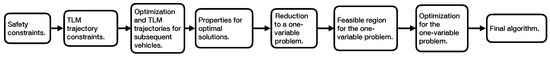
Figure 1.
Overview of methodology.
We assume n vehicles in a string formation (driving after each other on a road), where vehicle 1 or is the first vehicle that stops at the TL. This is shown in Figure 2. For each vehicle , the position (along the road) of the front of the vehicle is . Furthermore, we let be a position at some desired constant distance behind vehicle . If that constant distance is zero, this means that is the position of the rear end of vehicle . If the constant distance is larger than zero, this means that is a position behind the vehicle that is fixed in the coordinate frame of the vehicle. In the coordinate system of the TL, each vehicle i that has not passed the TL has negative coordinates and . As time progresses, the values of and increase and become positive as the vehicle passes the TL.
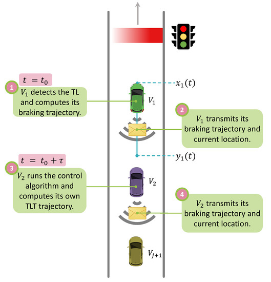
Figure 2.
System model.
Definition 1.
(Safety constraint). We define the system as safe when for for all . This means the system is deemed safe if each successive vehicle i is able to maintain a distance of at least away from its predecessor.
By choosing as a position strictly behind the vehicle allows for an additional safety margin. We assume that each vehicle i is described by the following dynamic model:
where and is the velocity and the acceleration of vehicle i, respectively.
Our aim is to develop a mechanism with which the string of vehicles may pass the TL efficiently while satisfying the safety conditions in Definition 1. Through a sequence of subsections, we provide the theory for such a mechanism, which is summarized as an algorithm in Section 4.7 at the end.
Formally, the TLM of is captured by Definition 2 further below (assuming without loss of generality that the time enters this mode is ). Besides specifying vehicle dynamics in TLM, Definition 2 also includes the safety constraint in Definition 1. This means that first decelerates with constant deceleration until time , then moves with constant velocity until time , then accelerates with constant acceleration until time , and then, as it enters Normal mode again, moves with constant velocity. The constants , and provide the upper bounds on deceleration, acceleration, and velocity, respectively.
The first vehicle, i.e., , might actually stop and stand still between the two given times and , where . In such cases, it decelerates with constant deceleration between times 0 and and accelerates with between times and , after which it drives with constant velocity. Given these conditions, our objective is to render the trajectories of subsequent vehicles, i.e., for , efficient.
Definition 2.
(Trajectory constraints for Traffic light mode (TLM)).
4.1. Distributed Optimization Problem
We propose a distributed approach using a predecessor-follower V2V communication topology. Each vehicle j selects its parameters based on those received from its predecessor vehicle . More specifically, the parameters , , , and are communicated from to and used to solve an optimization problem for the three parameters , and . In this optimization problem, we use an additional parameter , which captures communication as well as computational delays.
For , the objective f to be minimized subject to the constraints in Definition 2 is given by
where . The objective (2) is a convex combination of the deceleration magnitude during Phase 1 and an expression equivalent to the velocity (up to a constant) during Phase 2. The velocity during Phase 2 is equal to . Maximization of this entity is equivalent to minimization of . The main goal is to keep the trajectory of the vehicles as steady as possible by minimizing the overall changes in both acceleration and the traveling velocity. Doing so will essentially ensure that the time each successive vehicle comes to a full stop will be as short as possible while the overall system remains safe. Intuitively it promotes high throughput of vehicles at the TL.
We solve for the dynamical system (1) in TLM without loss of generality assuming the start time is 0 where we use the constraints in Definition 2, and obtain the “Trajectory for vehicle ” shown below in (3). We further assume that enters TLM at time . The instruction to enter TLM (with parameters) is sent with some latency or delay. On top of this delay comes additional computational delay. All such delays are captured by . This is the maximum difference between the time when enters TLM and the time when vehicle enters TLM. If vehicle enters TLM before time has passed everything is safe and trajectories are feasible. However, this cannot be guaranteed if enters TLM after time has passed. The choice of the parameters should reflect communication quality and computational capacity. Increasing results in worse performance with respect to objective (2) since a smaller time interval is left for trajectory planning.
With this delay , we define the constraints for the trajectory until the time for vehicle , referred to as “Trajectory of vehicle ” below (see (4)). Note again that in this context i is short hand notation for , i.e., is vehicle .
Trajectory for vehicle :
Trajectory for vehicle :
4.2. Properties for the Optimal Solutions
Proposition 1.
There are three cases for the optimal solution to (2) with subject to the constraints in Definition 2.
- 1.
- The optimal solution does not exist and no other solution exists, as there is no solution that satisfies the safety constraints in Definition 1. The problem is ill-posed.
- 2.
- The optimal solution is to choose .
- 3.
- For the optimal solution it holds that
Proof.
In the following, to simplify notation, we treat the parameters as dimensionless.
(1) Consider, for example, , , , , and . We have that .
(2) An example is when: , , , , , , . Optimal solutions are obtained by setting . This is illustrated in Figure 3.
(3) Now we assume assume the trajectory is feasible and further assume that that and (otherwise we would end up in a case equivalent to case (2) above). Assuming (5) and (6) do not hold for an optimal solution , we show that this assumption leads to a contradiction. Since the trajectory depends continuously on its parameters, we may decrease slightly and obtain a new feasible solution with smaller objective value. See Figure 4, where the claimed optimal solution, yellow, is improved to a better solution, green.

Figure 3.
The trajectory with , green, and feasible trajectories with , yellow, are below the trajectory of , blue, for all times. □

Figure 4.
The trajectory of for a feasible in green performs better than another feasible trajectory with a greater by a small value in yellow.
Proposition 2.
Let be an optimal solution for vehicle to (2) with subject to the constraints in Definition 2. The trajectory is described by the parameters where . Suppose and suppose is an alternative solution described by the parameters , and . All that differs between the trajectories is that the alternative solution has a smaller time-delay.
It holds that for
Proof.
For notational convenience, when comparing the two trajectories, we may think of the alternative trajectory as belonging to an alternative virtual vehicle . Thus, we will henceforth refer to the trajectory of and that of in the comparison.
Let . It holds that
We can show this by checking the solution for each time interval in (4). During the first time interval , neither of the vehicles and has started the braking process. Thus, the trajectories are identical.
We proceed with the time interval i.e., when is braking.
We see that equality holds.
We proceed with the time interval , i.e., when has finished the breaking maneuver and drives with constant velocity.
Again, equality holds. Now, it also holds that (since is upper bounding the velocity of vehicle ). Thus it follows that
4.3. Reduction to a Problem Involving Only
We now leverage the results in Section 4.2 in order to address the optimization problem in Section 4.1. The main focus will be on solutions of type 3) in Proposition 1. From such analysis, we also provide conditions for identification of cases (1) and (2) in Proposition 1. In the optimization problem, there are three free parameters or variables: . However, Proposition 1 case (3) provides constraints that allow reduction to only one variable. For this case we say that the trajectories “touch”. From a derivations perspective, the most suitable choice is to reduce the problem into one that only involves the variable . Once the problem has been reduced to a one-dimensional problem, an efficient local optimization procedure is used to solve it.
From these two equations, we obtain the expressions for and expressed as functions of .
4.4. Feasible Region for
In Section 4.3, we reduced the dimension of the optimization problem in Section 4.1 to a problem involving only the variable .
However, an important piece that is missing is how the constraints in Definition 2 translate to this one-dimensional representation of the optimization problem. We address this by using the expressions in Equations (9) and (10) in the constraints of Definition 2. The constraints from Definition 2 will be enumerated according to the order they are addressed below.
For each constraint k, we we obtain a lower or upper bound for the feasible region of the time interval where resides in the optimization problem. After all the ’s are computed, the feasible region is obtained by computing the maximum of the lower bounds and the minimum of the upper bounds among the ’s.
Constraint 1: .
Constraint 2: .
Constraint 3: .
Constraint 4: .
Constraint 5: .
where , .
Constraint 6: no crossing at the first segment. Besides the Constraints 1–5 above, we need to additionally ensure that during the time interval . If indeed during the time interval , it holds that the trajectory is feasible for all later points in time. A sufficient (however not necessary) condition is that which yields
4.5. Feasible Region for
The procedure of choosing should be applied only if where
The distance corresponds to the case when the trajectories touch even without a decelerating phase of the j-th vehicle. In other words, moving with initial constant velocity , the follower vehicle touches the preceding vehicle, and then the inter-vehicle distance (IVD) d increases again. If the distance is larger than , the adjustment of the velocity is not needed since the trajectories do not come to touch even in the worst case, i.e., when the j-th vehicle does not decelerate. The bound in (18) was received from Equations (7) and (8) under the assumption .
4.6. Optimization Procedure
Our objective is now to solve the following optimization problem:
(for some between 0 and 1) over the interval , where and . As previously mentioned, we want to minimize a convex combination of the deceleration and speed. By taking into account both the value and the rate of change of the velocity, we ensure each vehicle’s trajectory remains as close to its original path as possible.
One way to find the optimal value is to differentiate the cost function with respect to (after substituting the expressions of and from Section 4.3) and solve for . Thus, we resort to the gradient descent method which renders convergence to a local optimal solution quickly. Convergence is assumed when the difference in objective values for consecutive iterations has reach an -threshold. At each iteration, the value of is expressed as follows:
where k is the iteration, is the learning rate and is the derivative of the cost function f, respectively.
We differentiate above and obtain
4.7. Algorithm for Each Vehicle
Here we summarize our proposed procedure as an algorithm (see Algorithm 1 below) for each vehicle (for ) in the string of vehicles. Below we write (instead of i as before) as the index for the vehicle that preceeds vehicle j. Upon receiving a message from vehicle , vehicle employs the algorithm below to calculate the necessary deceleration time and amplitude. The message received from is assumed to contain the values of the following parameters: as well as a time stamp for the time the message was sent. By using the the time stamp, the time delay is calculated/chosen. The vehicle then computes its intended trajectory and sends the parameters of the trajectory to vehicle .
| Algorithm 1 Distributed V2V-based traffic lights passing |
|
5. Simulations
Algorithm 1 in Section 4.7 has been validated through MATLAB simulations as follows. We assume that vehicles enter a one lane road at a rate of 1200 vehicles per hour (i.e., a vehicle enters every 3 s). Each vehicle has a speed of . Without loss of generality, the first vehicle, denoted as , is assumed to enter at time . The vehicle drives for seconds and then starts slowing down with a deceleration magnitude until coming to a full stop at time . stops for a known period T (related to the duration of the TL red phase) and then starts accelerating at time with acceleration until it reaches its initial speed at time . Now, for any vehicle , when it starts decelerating it sends a message, via V2V communication, to the vehicle behind it. This message includes information about its planned trajectory. then uses the proposed algorithm to calculate its trajectory and acceleration values, which are sent to vehicle and so on. In the experiments, we assume that starts slowing down after s with = 12 m/s and stops for a period of . Communication between vehicles is assumed to be reliable with a delay of for a single packet to travel from a vehicle to subsequent one.
Figure 5 shows that using the proposed algorithm, vehicles can slow down and accelerate again safely. It is worth noting here that the touch point between consecutive vehicles occurs sequentially such that, for example, the first and second vehicles, denoted by , touch at around while the second vehicle and the third one, , touch at around . This shows that the algorithm can scale well to situations where the idle duration of the first vehicle is longer.
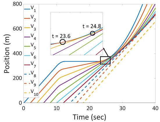
Figure 5.
Positions of ten consecutive vehicles.
Figure 6, on the other hand, shows the evolution of the vehicles’ velocities over time, starting from the moment the first vehicle starts decelerating. It can be observed that while the first vehicle decelerates to a velocity of , the rest of the vehicles decelerate and then move with a constant velocity before accelerating again. It is also depicted in the figure that vehicle keeps driving with the same speed and does not need to use the proposed optimization procedure.
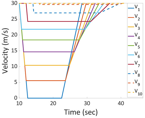
Figure 6.
Velocities of ten consecutive vehicles.
6. Conclusions and Discussion
The present paper proposes a distributed optimization procedure for safe and efficient passing of traffic lights for strings of vehicles. The procedure relies on predecessor–follower vehicle-to-vehicle (V2V) communication over the string of vehicles and is applicable to situations where the first vehicle (in the string) may (or may not) stop at the traffic light.
Each vehicle receives, via communication, a compact representation of the trajectory of its predecessor, which is used to compute a locally optimal solution for its own trajectory. The objective is to maximize a convex combination of minimum deceleration and minimum velocity, which promotes high energy efficiency and throughput. This is achieved, while ensuring safety in terms of no rear-end collisions. The computed trajectory is then subsequently passed on to the next (follower) vehicle.
The method is computationally efficient. Besides analytical expressions with constant computational time, the main computational complexity arises from a gradient descent procedure involving only one variable.
In terms of limitations, the proposed framework assumes vehicular dynamical models that are simple and explicitly solvable, excluding realistic nonlinear components. However, the proposed solutions still have potential to be used as worst-case solutions that bound the actual ones. The gap, in terms of performance, between the proposed solutions and the trajectories obtained for nonlinear vehicular dynamic models comprises an interesting future line of research to pursue.
An additional limitation is that the proposed method assumes trajectory-following without additional feedback. In essence, each vehicle computes a trajectory based on that communicated from the predecessor and is assumed to follow that trajectory during the passing of the traffic light. As a future extension to this procedure, one may consider re-computing and re-transmission of trajectories. Low computational complexity would allow for such a procedure in practice.
Lastly, in the presentation of the main procedure, it is assumed the velocities of involved vehicles are all constant and equal before entering traffic light mode where the algorithm is deployed. This is, however, not a necessary condition and may be relaxed to any type of initial velocity.
All-in-all, this new computationally efficient procedure provides a new perspective on cooperative vehicular coordination, which we believe would be of interest to the community.
Author Contributions
Conceptualization, J.T. and T.S.; Formal analysis, J.T. and G.S.; Funding acquisition, A.V.; Investigation, T.S. and F.V.; Methodology, J.T. and T.S.; Project administration, A.V.; Resources, T.S.; Software, T.S.; Supervision, J.T. and A.V.; Validation, T.S.; Visualization, T.S.; Writing—original draft, J.T., T.S., F.V. and A.V.; Writing—review and editing, J.T., F.V. and A.V. All authors have read and agreed to the published version of the manuscript.
Funding
This work was supported by the Swedish Knowledge Foundation (KKS) “Safety of Connected Intelligent Vehicles in Smart Cities—SafeSmart” project (2019–2024), the ELLIIT Strategic Research Network and the Helmholtz Program “Engineering Digital Futures”.
Data Availability Statement
All data were presented in the main text.
Conflicts of Interest
The authors declare no conflict of interest.
References
- Kopelias, P.; Demiridi, E.; Vogiatzis, K.; Skabardonis, A.; Zafiropoulou, V. Connected & autonomous vehicles—Environmental impacts—A review. Sci. Total Environ. 2020, 712, 135237. [Google Scholar] [CrossRef]
- Ye, L.; Yamamoto, T. Evaluating the impact of connected and autonomous vehicles on traffic safety. Phys. A Stat. Mech. Its Appl. 2019, 526, 121009. [Google Scholar] [CrossRef]
- Guo, G.; Zhao, Z.; Zhang, R. Distributed Trajectory Optimization and Fixed-Time Tracking Control of a Group of Connected Vehicles. IEEE Trans. Veh. Technol. 2023, 72, 1478–1487. [Google Scholar] [CrossRef]
- Bhattacharyya, K.; Laharotte, P.-A.; Burianne, A.; Faouzi, N.-E.E. Assessing Connected Vehicle’s Response to Green Light Optimal Speed Advisory From Field Operational Test and Scaling Up. IEEE Trans. Intell. Transp. Syst. 2022, 24, 6725–6736. [Google Scholar] [CrossRef]
- Vinel, A.; Koucheryavy, Y. On the delay lower bound for the emergency message dissemination in vehicular ad-hoc networks. In Proceedings of the 2009 IEEE 34th Conference on Local Computer Networks, Zurich, Switzerland, 20–23 October 2009; pp. 652–654. [Google Scholar] [CrossRef]
- Campolo, C.; Molinaro, A.; Berthet, A.O.; Vinel, A. On Latency and Reliability of Road Hazard Warnings over the Cellular V2X Sidelink Interface. IEEE Commun. Lett. 2019, 23, 2135–2138. [Google Scholar] [CrossRef]
- Naik, G.; Choudhury, B.; Park, J.-M. IEEE 802.11bd & 5G NR V2X: Evolution of Radio Access Technologies for V2X Communications. IEEE Access 2019, 7, 70169–70184. [Google Scholar] [CrossRef]
- Guo, G.; Li, P.; Hao, L.-Y. A New Quadratic Spacing Policy and Adaptive Fault-Tolerant Platooning with Actuator Saturation. IEEE Trans. Intell. Transp. Syst. 2022, 23, 1200–1212. [Google Scholar] [CrossRef]
- Prayitno, A.; Nilkhamhang, I. V2V Network Topologies for Vehicle Platoons with Cooperative State Variable Feedback Control. In Proceedings of the 2021 Second International Symposium on Instrumentation, Control, Artificial Intelligence, and Robotics (ICA-SYMP), Bangkok, Thailand, 18–20 January 2021; pp. 1–4. [Google Scholar] [CrossRef]
- Yu, W.; Hua, X.; Wang, W. Investigating the Longitudinal Impact of Cooperative Adaptive Cruise Control Vehicle Degradation Under Communication Interruption. IEEE Intell. Transp. Syst. Mag. 2022, 14, 183–201. [Google Scholar] [CrossRef]
- Thormann, S.; Schirrer, A.; Jakubek, S. Safe and Efficient Cooperative Platooning. IEEE Trans. Intell. Transp. Syst. 2022, 23, 1368–1380. [Google Scholar] [CrossRef]
- Sun, X.; Yu, F.R.; Zhang, P. A Survey on Cyber-Security of Connected and Autonomous Vehicles (CAVs). IEEE Trans. Intell. Transp. Syst. 2022, 23, 6240–6259. [Google Scholar] [CrossRef]
- Sander, U.; Lubbe, N.; Pietzsch, S. Intersection AEB implementation strategies for left turn across path crashes. Traffic Inj. Prev. 2019, 20 (Suppl. S1), S119–S125. [Google Scholar] [CrossRef]
- Elliott, D.; Keen, W.; Miao, L. Recent advances in connected and automated vehicles. J. Traffic Transp. Eng. 2019, 6, 109–131. [Google Scholar] [CrossRef]
- Sidorenko, G.; Fedorov, A.; Thunberg, J.; Vinel, A. Towards a Complete Safety Framework for Longitudinal Driving. IEEE Trans. Intell. Veh. 2022, 7, 809–814. [Google Scholar] [CrossRef]
- Guo, G.; Wang, Q. Fuel-Efficient En Route Speed Planning and Tracking Control of Truck Platoons. IEEE Trans. Intell. Transp. Syst. 2019, 20, 3091–3103. [Google Scholar] [CrossRef]
- Guo, G.; Li, P.; Hao, L.-Y. Adaptive Fault-Tolerant Control of Platoons with Guaranteed Traffic Flow Stability. IEEE Trans. Veh. Technol. 2020, 69, 6916–6927. [Google Scholar] [CrossRef]
- Feng, S.; Zhang, Y.; Li, S.E.; Cao, Z.; Liu, H.X.; Li, L. String stability for vehicular platoon control: Definitions and analysis methods. Annu. Rev. Control 2019, 47, 81–97. [Google Scholar] [CrossRef]
- Chien, C.C.; Ioannou, P. Automatic Vehicle-Following. In Proceedings of the 1992 American Control Conference, Chicago, IL, USA, 24–26 June 1992; pp. 1748–1752. [Google Scholar] [CrossRef]
- Sungu, H.E.; Inoue, M.; Imura, J.-I. Nonlinear spacing policy based vehicle platoon control for local string stability and global traffic flow stability. In Proceedings of the 2015 European Control Conference (ECC), Linz, Austria, 15–17 July 2015; pp. 3396–3401. [Google Scholar] [CrossRef]
- Koopman, P.; Osyk, B.; Weast, J. Autonomous Vehicles Meet the Physical World: RSS, Variability, Uncertainty, and Proving Safety. In Computer Safety, Reliability, and Security, Proceedings of the SAFECOMP 2019, Turku, Finland, 11–13 September 2019; Romanovsky, A., Troubitsyna, E., Bitsch, F., Eds.; Lecture Notes in Computer Science; Springer: Cham, Switzerland, 2019; Volume 11698. [Google Scholar] [CrossRef]
- Vinel, A.; Lyamin, N.; Isachenkov, P. Modeling of V2V Communications for C-ITS Safety Applications: A CPS Perspective. IEEE Commun. Lett. 2018, 22, 1600–1603. [Google Scholar] [CrossRef]
- Fu, Y.; Li, C.; Yu, F.R.; Luan, T.H.; Zhang, Y. A Decision-Making Strategy for Vehicle Autonomous Braking in Emergency via Deep Reinforcement Learning. IEEE Trans. Veh. Technol. 2020, 69, 5876–5888. [Google Scholar] [CrossRef]
- Meng, Y.; Li, L.; Wang, F.-Y.; Li, K.; Li, Z. Analysis of Cooperative Driving Strategies for Nonsignalized Intersections. IEEE Trans. Veh. Technol. 2018, 67, 2900–2911. [Google Scholar] [CrossRef]
- Stern, R.E.; Cui, S.; Delle Monache, M.L.; Bhadani, R.; Bunting, M.; Churchill, M.; Hamilton, N.; Haulcy, R.; Pohlmann, H.; Wu, F.; et al. Dissipation of stop-and-go waves via control of autonomous vehicles: Field experiments. Transp. Res. Part C Emerg. Technol. 2018, 89, 205–221. [Google Scholar] [CrossRef]
- Meng, X.; Cassandras, C.G. Eco-Driving of Autonomous Vehicles for Nonstop Crossing of Signalized Intersections. IEEE Trans. Autom. Sci. Eng. 2022, 19, 320–331. [Google Scholar] [CrossRef]
- Guo, L.; Chu, H.; Ye, J.; Gao, B.; Chen, H. Hierarchical Velocity Control Considering Traffic Signal Timings for Connected Vehicles. IEEE Trans. Intell. Veh. 2023, 8, 1403–1414. [Google Scholar] [CrossRef]
- Ye, L.; Yamamoto, T. Impact of dedicated lanes for connected and autonomous vehicle on traffic flow throughput. Phys. A Stat. Mech. Its Appl. 2018, 512, 588–597. [Google Scholar] [CrossRef]
- Valle, F.; Vinel, A.; Erneberg, M. Traffic Light Priority in NordicWay. Communication Technologies for Vehicles. Nets4Cars/Nets4Trains/Nets4Aircraft 2021, 2021, 49–55. [Google Scholar] [CrossRef]
Disclaimer/Publisher’s Note: The statements, opinions and data contained in all publications are solely those of the individual author(s) and contributor(s) and not of MDPI and/or the editor(s). MDPI and/or the editor(s) disclaim responsibility for any injury to people or property resulting from any ideas, methods, instructions or products referred to in the content. |
© 2023 by the authors. Licensee MDPI, Basel, Switzerland. This article is an open access article distributed under the terms and conditions of the Creative Commons Attribution (CC BY) license (https://creativecommons.org/licenses/by/4.0/).