


Optimizing Intrusion Detection Systems in Three Phases on the CSE-CIC-IDS-2018 Dataset


Abstract
:1. Introduction
- Investigation of large amounts of data linked with harmful network activity;
- Identification of feature dimensions influencing classification performance in a labeled dataset with both benign and malicious traffic, resulting in improved detection accuracy;
- Use of the CSE-CIC-IDS-2018 dataset for NIDS and testing of seven different machine learning classifiers and scripts for identifying various sorts of assaults;
- In general, researchers frequently work with incomplete data. In contrast, this study uses all accessible DDoS data in the experiment, correlating with reality by adopting the concept of data imbalance;
- Presenting various performance assessments has many elements. Furthermore, the evaluation considers CPU processing time, which is an important component in intrusion detection, as well as the size of the experimentally obtained model, which has the possibility for future extension.
2. Related Work
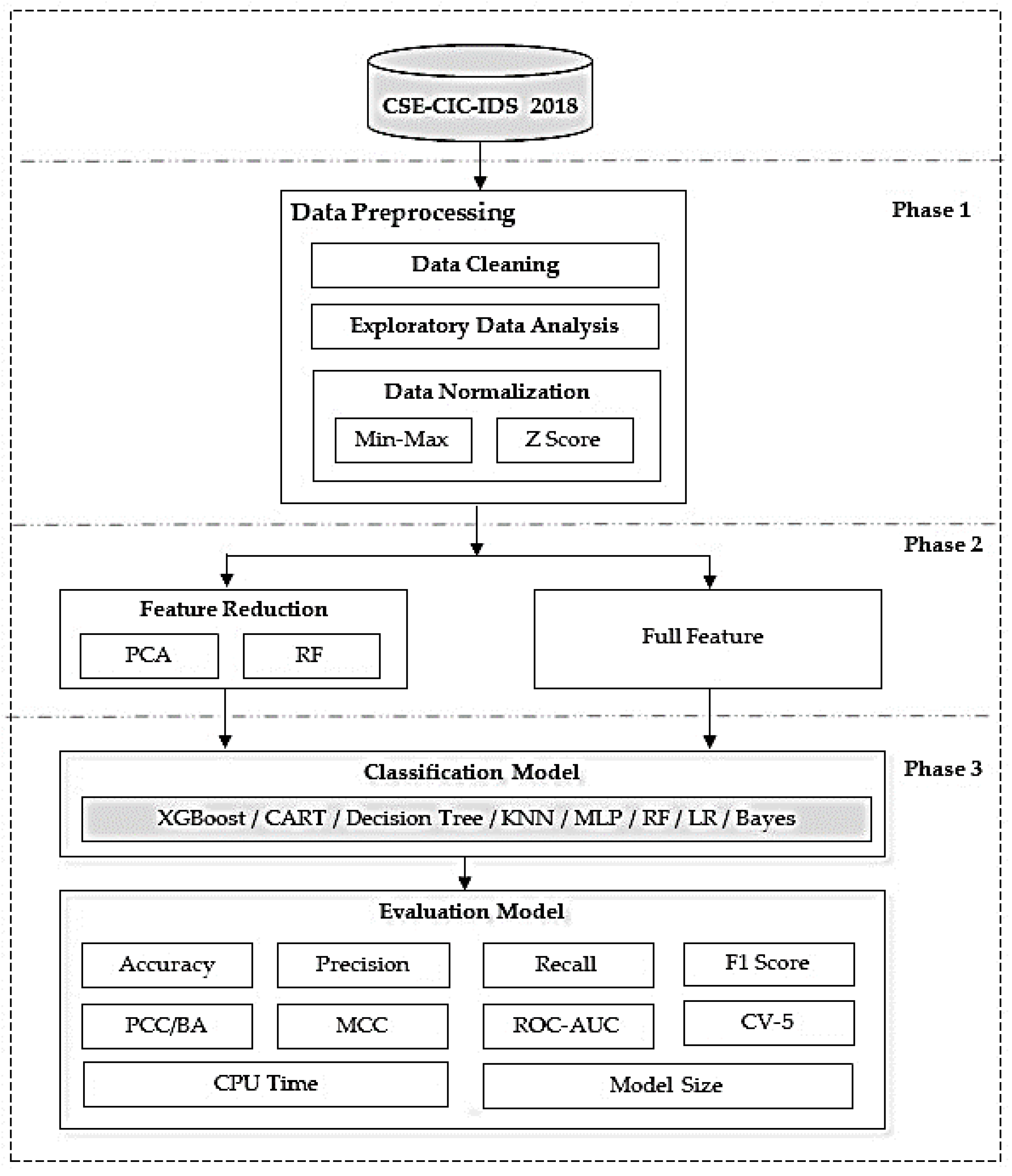
3. Methods
4. Experimental Setup
4.1. CSE-CIC-IDS-2018 Data Set
4.2. Data Preprocessing
4.2.1. Data Cleaning
4.2.2. Exploratory Data Analysis
4.2.3. Data Normalization
- Min–Max Normalization: This approach reduces the values of a feature to a range between 0 and 1. It accomplishes this by subtracting the minimum value of the feature from each data point and then dividing the result by the range of the feature. This technique’s equivalent mathematical equation is shown as (1), where X is an original value and X′ is the normalized value [35]:
- Z-score Normalization: This method scales a feature’s values to have a mean of 0 and a standard deviation of 1. This is accomplished by removing the feature’s mean from each value and then dividing by the standard deviation. Mathematical equation for this strategy is given as (2), where X is an original value and X′ is the normalized value [36]:
4.3. Feature Selection
4.3.1. PCA
4.3.2. RF
4.4. Classification Model
4.4.1. XGBoost
4.4.2. CART
4.4.3. DT
4.4.4. KNN
4.4.5. Multilayer Perceptron (MLP)
4.4.6. RF
4.4.7. LR
4.4.8. Bayes
4.5. Evaluation Model
- F1 score contains both recall and precision and the mathematical equation for this strategy is given as (3)The F1 score provides more weight to the lower of the two values and is the harmonic mean of precision and recall. This indicates that if either precision or recall is low, the F1 score will be much lower as well. However, if both precision and recall are strong, the F1 score will be close to 1. This can result in a biased outcome if one of the measurements is significantly greater than the other [4].
- The Matthews correlation coefficient (MCC) is a more reliable statistical rate that produces a high score only if the prediction performed well in all four confusion matrix categories (true positives, false negatives, true negatives, and false positives), proportionally to the size of positive and negative elements in the dataset. MCC’s formula takes into account all of the cells in the confusion matrix. In machine learning, the MCC is used to assess the quality of binary (2-class) classification. MCC is a correlation coefficient that exists between the exact and projected binary classifications and typically returns a value of 0 or 1. mathematical equation for this strategy is given as (4) [38], where TP as correctly predicted positives are called true positives, FN as wrongly predicted negatives are called false negatives, TN actual negatives that are correctly predicted negatives are called true negatives, and FP actual negatives that are wrongly predicted positives are called false positives:
- Receiver operating characteristic (ROC) as most indicators can be influenced by dataset class imbalance, making it difficult to rely on a single indication for model differentiation [39]. ROC curves are used to differentiate between attack and benign instances, with the x-axis representing the false alarm rate (FAR) and the y-axis representing the detection rate (DR).
- The probability of correct classification (PCC) is a probability value between 0 and 1 that examines the classifier’s ability to detect certain classes. It is critical to understand that relying only on overall accuracy across positive and negative examples might be misleading. Even if our training data is balanced, performance disparities in different production batches are possible. As a result, accuracy alone is not a reliable measure, emphasizing the need of metrics such as PCC, which focus on the classifier’s accurate classification probabilities for individual classes.
- Balanced accuracy (BA) is calculated as the average of sensitivity and specificity, or the average of the proportion corrects of each individually. It entails categorizing the data into two categories. The mathematical equation for this strategy is given as (5). When all classes are balanced, so that each class has the same TN number of samples, TP + FN TN + FP and binary classifier’s “regular” accuracy is approximately equivalent to balanced accuracy:
- ROC score handled the case of a few negative labels similar to the case of a few positive labels. It is worth noting that the F1 score for the model is nearly the same because positive labels are plentiful, and it only cares about positive label misclassification. The probabilistic explanation of the ROC score is that a positive example and a negative case are chosen at random. In this case, rank is defined by the order of projected values.
- Cross-validation (CV) is a statistic used to evaluate the performance of a machine learning model. The dataset is partitioned into k subsets or folds in k-fold cross-validation. The model is trained on one of these folds while being validated on the others. This procedure is performed k times, with each fold only serving as validation data once. To measure total accuracy, the accuracy ratings acquired from each fold are averaged. This method ensures that the model is evaluated over numerous data subsets, reducing the danger of overfitting and producing a more realistic estimate of its performance on unseen data.
- In the context of evaluation, CPU time refers to the overall length of time it takes a CPU to complete a certain job or process. When analyzing algorithms or models, CPU time is critical for determining computational efficiency. Evaluating CPU time helps determine how quickly a given algorithm or model processes data, making it useful for optimizing performance, particularly in applications where quick processing is required, such as real-time systems or large-scale data processing jobs. Lower CPU time indicates faster processing and is frequently used to determine the efficiency and practical applicability of algorithms or models.
- The memory space occupied by a machine learning model when deployed for prediction tasks is referred to as model size in classification. Model size must be considered, especially in applications with limited storage capacity, such as mobile devices or edge computing environments. A lower model size is helpful since it minimizes memory requirements, allowing for faster loading times and more efficient resource utilization. However, it is critical to strike a balance between model size and forecast accuracy; highly compressed models may forfeit accuracy. As a result, analyzing model size assures that the deployed classification system is not only accurate but also suited for the given computer environment, hence increasing its practicality and usability.
5. Experimental Results and Discussions
6. Conclusions
Author Contributions
Funding
Data Availability Statement
Conflicts of Interest
References
- Momand, A.; Jan, S.U.; Ramzan, N. A Systematic and Comprehensive Survey of Recent Advances in Intrusion Detection Systems Using Machine Learning: Deep Learning, Datasets, and Attack Taxonomy. J. Sens. 2023, 2023, 6048087. [Google Scholar] [CrossRef]
- Aljanabi, M.; Ismail, M.A.; Ali, A.H. Intrusion detection systems, issues, challenges, and needs. Int. J. Comput. Intell. Syst. 2021, 14, 560–571. [Google Scholar] [CrossRef]
- Qusyairi, R.; Saeful, F.; Kalamullah, R. Implementation of Ensemble Learning and Feature Selection for Performance Improvements in Anomaly-Based Intrusion Detection Systems. In Proceedings of the International Conference on Industry 4.0, Artificial Intelligence, and Communications Technology (IAICT), Bali, Indonesia, 7–8 July 2020. [Google Scholar]
- Chimphlee, S.; Chimphlee, W. Machine learning to improve the performance of anomaly-based network intrusion detection in big data. Indones. J. Electr. Eng. Comput. Sci. 2023, 30, 1106–1119. [Google Scholar] [CrossRef]
- Kaja, N.; Shaout, A.; Ma, D. An intelligent intrusion detection system. Appl. Intell. 2019, 49, 3235–3247. [Google Scholar] [CrossRef]
- Umar, M.A.; Chen, Z. Effects of Feature Selection and Normalization on Network Intrusion Detection. TechRxiv 2020. preprint. [Google Scholar] [CrossRef]
- Jaradat, A.S.; Barhoush, M.M.; Easa, R.B. Network intrusion detection system: Machine learning approach. Indones. J. Electr. Eng. Comput. Sci. 2022, 25, 1151–1158. [Google Scholar] [CrossRef]
- Gautam, R.K.S.; Doegar, E.A. An Ensemble Approach for Intrusion Detection System Using Machine Learning Algorithms. In Proceedings of the 2018 8th International Conference on Cloud Computing, Data Science & Engineering, Noida, India, 11–12 January 2018. [Google Scholar]
- Nassif, A.B.; Talib, M.A.; Nasir, Q.; Dakalbab, F.M. Machine Learning for Anomaly Detection: A Systematic Review. IEEE Access 2021, 9, 78658–78700. [Google Scholar] [CrossRef]
- Kim, J.; Shin, Y.; Choi, E. An Intrusion Detection Model based on a Convolutional Neural Network. J. Multimed. Inf. Syst. 2019, 6, 165–172. [Google Scholar] [CrossRef]
- Karatas, G.; Demir, O.; Sahingoz, O.K. Increasing the Performance of Machine Learning-Based IDSs on an Imbalanced and Up-to-Date Dataset. IEEE Access 2020, 8, 32150–32162. [Google Scholar] [CrossRef]
- Ambusaidi, M.A.; He, X.; Nanda, P.; Tan, Z. Building an intrusion detection system using a filter-based feature selection algorithm. IEEE Trans. Comput. 2016, 65, 2986–2998. [Google Scholar] [CrossRef]
- Muhsen, A.R.; Jumaa, G.G.; Bakri, N.F.A.; Sadiq, A.T. Feature Selection Strategy for Network Intrusion Detection System (NIDS) Using Meerkat Clan Algorithm. Int. J. Interact. Mob. Technol. 2021, 15, 158–171. [Google Scholar] [CrossRef]
- Ullah, S.; Mahmood, Z.; Ali, N.; Ahmad, T.; Buriro, A. Machine Learning-Based Dynamic Attribute Selection Technique for DDoS Attack Classification in IoT Networks. Computers 2023, 12, 115. [Google Scholar] [CrossRef]
- Khan, M.A. HCRNNIDS: Hybrid convolutional recurrent neural network-based network intrusion detection system. Processes 2021, 9, 834. [Google Scholar] [CrossRef]
- Padmashree, A.; Krishnamoorthi, M. Decision Tree with Pearson Correlation-based Recursive Feature Elimination Model for Attack Detection in IoT Environment. Inf. Technol. Control 2022, 51, 771–785. [Google Scholar] [CrossRef]
- Malliga, S.; Nandhini, P.S.; Kogilavani, S.V. A Comprehensive Review of Deep Learning Techniques for the Detection of (Distributed) Denial of Service Attacks. Inf. Technol. Control 2022, 51, 180–215. [Google Scholar] [CrossRef]
- Alzaqebah, A.; Aljarah, I.; Al-Kadi, O.; Damaševičius, R. A Modified Grey Wolf Optimization Algorithm for an Intrusion Detection System. Mathematics 2022, 10, 999. [Google Scholar] [CrossRef]
- Toldinas, J.; Venčkauskas, A.; Damaševičius, R.; Grigaliūnas, Š.; Morkevičius, N.; Baranauskas, E. A novel approach for network intrusion detection using multistage deep learning image recognition. Electronics 2021, 10, 1854. [Google Scholar] [CrossRef]
- Damasevicius, R.; Venckauskas, A.; Grigaliunas, S.; Toldinas, J.; Morkevicius, N.; Aleliunas, T.; Smuikys, P. Litnet-2020: An annotated real-world network flow dataset for network intrusion detection. Electronics 2020, 9, 800. [Google Scholar] [CrossRef]
- Ali, M.H.; Jaber, M.M.; Abd, S.K.; Rehman, A.; Awan, M.J.; Damaševičius, R.; Bahaj, S.A. Threat Analysis and Distributed Denial of Service (DDoS) Attack Recognition in the Internet of Things (IoT). Electronics 2022, 11, 494. [Google Scholar] [CrossRef]
- Leevy, J.L.; Khoshgoftaar, T.M. A survey and analysis of intrusion detection models based on CSE-CIC-IDS2018 Big Data. J. Big Data 2020, 7, 104. [Google Scholar] [CrossRef]
- Nskh, P.; Varma, M.N.; Naik, R.R. Principle component analysis based intrusion detection system using support vector machine. Proceedings of 2016 IEEE International Conference on Recent Trends in Electronics, Information & Communication Technology (RTEICT), Bangalore, India, 20–21 May 2016; pp. 1344–1350. [Google Scholar] [CrossRef]
- Hasan, M.A.M.; Nasser, M.; Ahmad, S.; Molla, K.I. Feature Selection for Intrusion Detection Using Random Forest. J. Inf. Secur. 2016, 7, 129–140. [Google Scholar] [CrossRef]
- Dhaliwal, S.S.; Al Nahid, A.; Abbas, R. Effective intrusion detection system using XGBoost. Information 2018, 9, 149. [Google Scholar] [CrossRef]
- Radoglou-Grammatikis, P.I.; Sarigiannidis, P.G. An Anomaly-Based Intrusion Detection System for the Smart Grid Based on CART Decision Tree. In Proceedings of the 2018 Global Information Infrastructure and Networking Symposium (GIIS), Thessaloniki, Greece, 23–25 October 2018; pp. 1–5. [Google Scholar] [CrossRef]
- Shilpashree, S.; Lingareddy, S.C.; Bhat, N.G.; Kumar, G.S. Decision tree: A machine learning for intrusion detection. Int. J. Innov. Technol. Explor. Eng. 2019, 8, 1126–1130. [Google Scholar] [CrossRef]
- Wazirali, R. An Improved Intrusion Detection System Based on KNN Hyperparameter Tuning and Cross-Validation. Arab. J. Sci. Eng. 2020, 45, 10859–10873. [Google Scholar] [CrossRef]
- Jamal, E.; Reza, M.; Jamal, G. Intrusion Detection System Based on Multi-Layer Perceptron Neural Networks and Decision Tree. In Proceedings of the International Conference on Information and Knowledge Technology, Urmia, Iran, 26–28 May 2015. [Google Scholar]
- Farnaaz, N.; Jabbar, M.A. Random Forest Modeling for Network Intrusion Detection System. Procedia Comput. Sci. 2016, 89, 213–217. [Google Scholar] [CrossRef]
- Ghosh, P.; Mitra, R. Proposed GA-BFSS and logistic regression based intrusion detection system. In Proceedings of the 2015 Third International Conference on Computer, Communication, Control and Information Technology (C3IT), Hooghly, India, 7–8 February 2015; pp. 1–6. [Google Scholar] [CrossRef]
- Sharmila, B.S.; Nagapadma, R. Intrusion Detection System using Naive Bayes algorithm. In Proceedings of the 2019 IEEE International WIE Conference on Electrical and Computer Engineering (WIECON-ECE), Bangalore, India, 15–16 September 2019; pp. 1–4. [Google Scholar] [CrossRef]
- Li, W.; Liu, Z. A method of SVM with normalization in intrusion detection. Procedia Environ. Sci. 2011, 11, 256–262. [Google Scholar] [CrossRef]
- Ketepalli, G.; Bulla, P. Data Preparation and Pre-processing of Intrusion Detection Datasets using Machine Learning. In Proceedings of the 2023 International Conference on Inventive Computation Technologies (ICICT), Lalitpur, Nepal, 26–28 April 2023; pp. 257–262. [Google Scholar] [CrossRef]
- Eslamnezhad, M.; Varjani, A.Y. Intrusion detection based on MinMax K-means clustering. In Proceedings of the 7’th International Symposium on Telecommunications (IST’2014), Tehran, Iran, 9–11 September 2014; pp. 804–808. [Google Scholar] [CrossRef]
- Zeng, Z.; Peng, W.; Zhao, B. Improving the Accuracy of Network Intrusion Detection with Causal Machine Learning. Secur. Commun. Netw. 2021, 2021, 8986243. [Google Scholar] [CrossRef]
- Le, T.T.H.; Kim, H.; Kang, H.; Kim, H. Classification and Explanation for Intrusion Detection System Based on Ensemble Trees and SHAP Method. Sensors 2022, 22, 1154. [Google Scholar] [CrossRef]
- Chicco, D.; Jurman, G. The advantages of the Matthews correlation coefficient (MCC) over F1 score and accuracy in binary classification evaluation. BMC Genom. 2020, 21, 6. [Google Scholar] [CrossRef]
- Sarhan, M.; Layeghy, S.; Moustafa, N.; Gallagher, M.; Portmann, M. Feature extraction for machine learning-based intrusion detection in IoT networks. Digit. Commun. Netw. 2022, in press. [Google Scholar] [CrossRef]


| Study | Methodology/Findings |
|---|---|
| S. Ullah. et al. [14] | Compares machine learning algorithms (RF, Bayes, LR, KNN, DT) and feature selection by RF (30 features) using CSE-CIC-IDS-2018 dataset. DT yielded the best results. |
| M. A. Khan. [15] | Develops HCRNNIDS, a hybrid convolutional recurrent neural network-based NIDS, and compares it with machine learning algorithms (DT, LR, XGBoost) and feature selection by RF (30 features) using CSE-CIC-IDS-2018 dataset. HCRNNIDS showed superior results. |
| J. Kim. et al. [10] | Discusses IDS models using various machine learning algorithms (ANN, SVM, CNN, RNN) and finds that CNN outperforms traditional techniques when applied to CSE-CIC-IDS-2018 dataset. |
| R. Qusyairi. et al. [3] | Proposes an ensemble learning technique incorporating LR, DT, and gradient boosting after comparisons with single classifiers, using the CSE-CIC-IDS-2018 dataset. Identified 23 significant traits out of 80. |
| S. Chimphlee. et al. [4] | Focuses on IDS using the CSE-CIC-IDS-2018 dataset, employs data preprocessing, feature selection, and seven classifier machine learning algorithms (including MLP and XGBoost). MLP provided the most successful outcomes. |
| A. Padmashree. et al. [16] | Addresses the industrial revolution’s IoT security challenges by offering a robust model with efficient feature selection, preprocessing, and DT-PCRFE for increased security. The model achieves a stunning 99.2% accuracy using word embeddings and a DNN, which is critical for protecting IoT devices in smart city expansion. |
| S. Malliga. et al. [17] | Looks at denial of service (DoS/DDoS) attacks, focusing on how attack patterns evolve. It examines contemporary deep-learning-based detection algorithms since 2016, classifies attack types, and assesses datasets. The findings indicate the need for improved techniques to dealing with dynamic attacker behavior, noting gaps in the existing literature and recommending future research directions. |
| A. Alzaqebah. et al. [18] | Improves network intrusion detection systems by employing a modified grey wolf optimization algorithm, with a focus on enhanced detection of regular and anomalous traffic. With an accuracy of 81%, an F1 score of 78%, and a G-mean of 84%, the strategy combines filter and wrapper strategies to produce excellent performance, notably in decreasing error rates. The model beats previous meta-heuristic algorithms when tested on the UNSWNB-15 dataset. |
| J. Toldinas. et al. [19] | Describes a novel approach for detecting network intrusions using multistage deep learning image recognition. The suggested method achieves exceptional accuracies of 99.8% for generic attack identification on UNSW-NB15 and 99.7% for DDoS and normal traffic detection on BOUN DDoS by transforming network features into four-channel pictures and leveraging the ResNet50 model. |
| R. Damasevicius. et al. [20] | Introduces LITNET-2020, a novel annotated network benchmark dataset derived from a real-world academic network, addressing the scarcity of realistic datasets for network intrusion detection. With 85 network flow features and 12 attack types, the dataset proves effective in identifying different attack classes, providing a valuable resource for research purposes. |
| M. H. Ali. et al. [21] | Addresses IoT security using a sparse convolutional network for intrusion detection, focusing on DDoS attacks. Trained with intrusion data and characteristics, the network is optimized using evolutionary techniques, effectively minimizing intrusion involvement in IoT data transmission. Experimental results demonstrate superior network security compared with traditional methods. |
| Type | Original Data | After Clean Data | ||
|---|---|---|---|---|
| Label Feature | Record | Percent | Record | Percent |
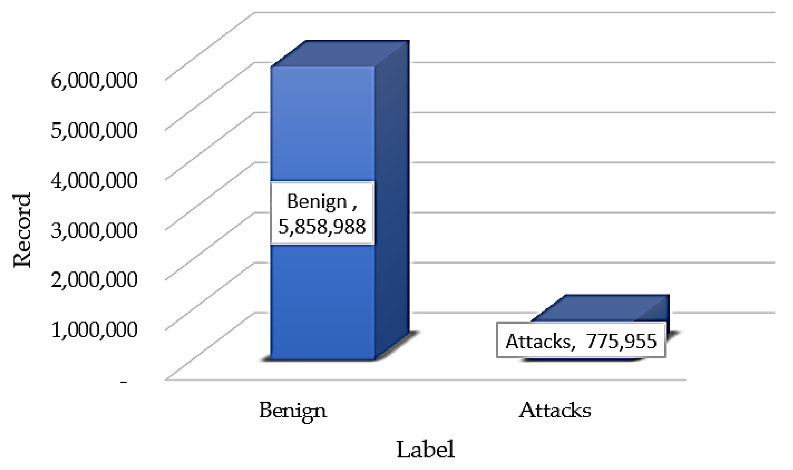
| Benign | 7,733,390 | 85.95 | 5,858,988 | 88.31 |
| DoS attacks-LOIC-HTTP | 576,191 | 6.40 | 575,364 | 8.67 |
| DDOS attack-HOIC | 686,012 | 7.62 | 198,861 | 3.00 |
| DDOS attack-LOIC-UDP | 1730 | 0.02 | 1730 | 0.03 |
| total | 8,997,323 | 100.00 | 6,634,943 | 100.00 |
| Classifiers | Accuracy | Precision | Recall | F1 Score | PCC/BA | MCC | ROC | CV 5 | CPU Time (S) | Model Size (KB) |
|---|---|---|---|---|---|---|---|---|---|---|
| Min–Max | ||||||||||
| XGBoost | 0.999950 | 0.975427 | 0.982578 | 0.978946 | 0.982578 | 0.999765 | 0.991281 | 0.999930 | 92.86 | 590.85 |
| CART | 0.999917 | 0.967775 | 0.960877 | 0.964270 | 0.960877 | 0.999609 | 0.980424 | 0.997995 | 112.79 | 57.31 |
| DT | 0.999911 | 0.958447 | 0.960853 | 0.959643 | 0.960853 | 0.999580 | 0.980413 | 0.999889 | 65.41 | 68.74 |
| RF | 0.999631 | 0.956304 | 0.982593 | 0.968626 | 0.982593 | 0.998260 | 0.991064 | 0.999560 | 131.67 | 7860.20 |
| Bayes | 0.950489 | 0.747992 | 0.984988 | 0.831505 | 0.984988 | 0.820660 | 0.986005 | 0.950566 | 7.02 | 6.65 |
| LR | 0.992956 | 0.898140 | 0.989497 | 0.937082 | 0.989497 | 0.967303 | 0.992159 | 0.989964 | 860.09 | 4.58 |
| MLP | 0.999835 | 0.938870 | 0.993869 | 0.962856 | 0.993869 | 0.999221 | 0.996879 | 0.998905 | 2220.53 | 291.93 |
| KNN | 0.999848 | 0.947640 | 0.963627 | 0.955322 | 0.963627 | 0.999281 | 0.981772 | 0.999815 | 6460.54 | 2,861,321.35 |
| Z-score | ||||||||||
| XGBoost | 0.999948 | 0.977524 | 0.977526 | 0.977525 | 0.977526 | 0.999755 | 0.988754 | 0.999934 | 89.12 | 581.15 |
| CART | 0.999921 | 0.968903 | 0.964489 | 0.966674 | 0.964489 | 0.999626 | 0.982229 | 0.997749 | 151.42 | 56.89 |
| DT | 0.999918 | 0.960671 | 0.967360 | 0.963963 | 0.967360 | 0.999612 | 0.983669 | 0.999881 | 76.50 | 68.93 |
| RF | 0.999739 | 0.966118 | 0.982353 | 0.973918 | 0.982353 | 0.998769 | 0.991008 | 0.999603 | 153.25 | 17,055.20 |
| Bayes | 0.949471 | 0.752121 | 0.984739 | 0.834724 | 0.984739 | 0.817708 | 0.985739 | 0.950838 | 7.43 | 6.65 |
| LR | 0.996893 | 0.912855 | 0.994199 | 0.947252 | 0.994199 | 0.985584 | 0.996643 | 0.995351 | 6920.85 | 4.58 |
| MLP | 0.998974 | 0.923494 | 0.998375 | 0.954336 | 0.998375 | 0.995160 | 0.998676 | 0.998805 | 1167.41 | 291.81 |
| KNN | 0.999840 | 0.945759 | 0.967207 | 0.955923 | 0.967207 | 0.999246 | 0.983554 | 0.999803 | 11,468.02 | 2,861,321.35 |
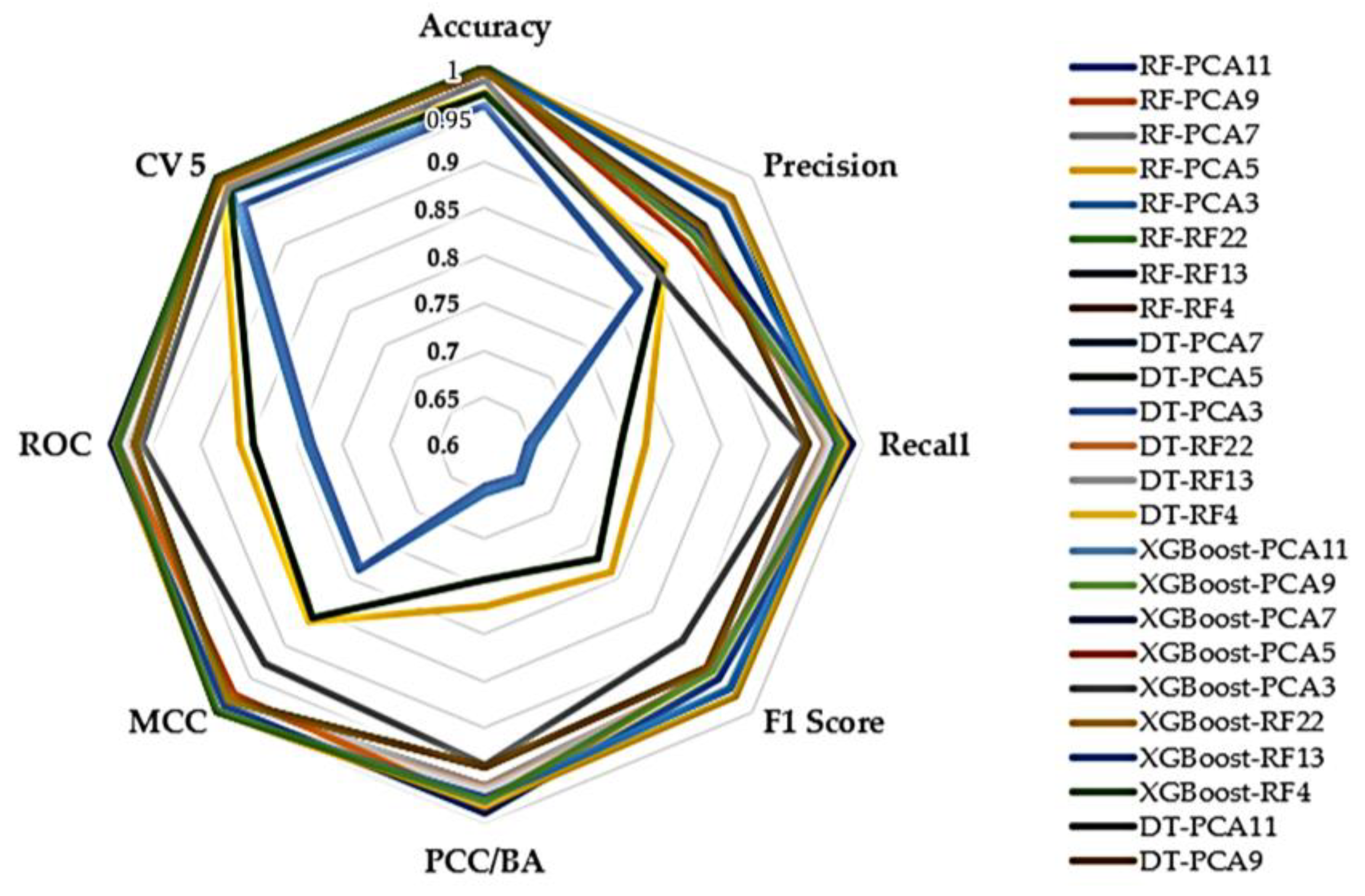
| Classifiers | Accuracy | Precision | Recall | F1 Score | PCC/BA | MCC | ROC | CV 5 | CPU Time (S) | Model Size (KB) |
|---|---|---|---|---|---|---|---|---|---|---|
| Min-Max | ||||||||||
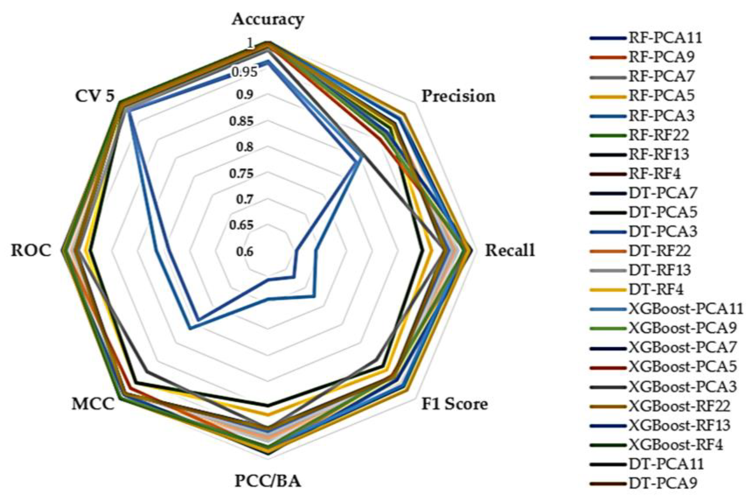
| RF-PCA11 | 0.996154 | 0.925325 | 0.960638 | 0.942236 | 0.960638 | 0.982109 | 0.979327 | 0.997329 | 135.52 | 31,307.31 |
| RF-PCA9 | 0.996145 | 0.926899 | 0.960586 | 0.943059 | 0.960586 | 0.982067 | 0.979291 | 0.997325 | 131.46 | 31,335.76 |
| RF-PCA7 | 0.996159 | 0.927997 | 0.960655 | 0.943677 | 0.960655 | 0.982134 | 0.979337 | 0.997324 | 137.16 | 31,305.15 |
| RF-PCA5 | 0.972420 | 0.869089 | 0.770071 | 0.789002 | 0.770071 | 0.863637 | 0.859193 | 0.991191 | 168.64 | 55,616.56 |
| RF-PCA3 | 0.958392 | 0.832067 | 0.652148 | 0.655230 | 0.652148 | 0.788547 | 0.787589 | 0.977432 | 197.05 | 334,645.57 |
| RF-RF22 | 0.999870 | 0.955205 | 0.975940 | 0.965073 | 0.975940 | 0.999385 | 0.987934 | 0.999761 | 188.84 | 10,281.29 |
| RF-RF13 | 0.999920 | 0.960641 | 0.970969 | 0.965681 | 0.970969 | 0.999623 | 0.985472 | 0.999881 | 154.06 | 5400.85 |
| RF-RF4 | 0.999837 | 0.913762 | 0.983025 | 0.942297 | 0.983025 | 0.999232 | 0.991467 | 0.999819 | 129.30 | 1241.54 |
| DT-PCA11 | 0.996097 | 0.925248 | 0.940889 | 0.932627 | 0.940889 | 0.981836 | 0.969390 | 0.997278 | 8.67 | 1173.92 |
| DT-PCA9 | 0.996098 | 0.925831 | 0.940891 | 0.932914 | 0.940891 | 0.981840 | 0.969392 | 0.997278 | 6.77 | 1174.43 |
| DT-PCA7 | 0.996099 | 0.925985 | 0.941614 | 0.933358 | 0.941614 | 0.981843 | 0.969753 | 0.997283 | 6.20 | 1174.20 |
| DT-PCA5 | 0.971348 | 0.861854 | 0.743431 | 0.769738 | 0.743431 | 0.858021 | 0.844684 | 0.981260 | 5.35 | 2028.59 |
| DT-PCA3 | 0.957864 | 0.829175 | 0.643716 | 0.647520 | 0.643716 | 0.785412 | 0.782492 | 0.959822 | 5.95 | 12,713.26 |
| DT-RF22 | 0.999918 | 0.961201 | 0.963030 | 0.962111 | 0.963030 | 0.999612 | 0.981504 | 0.999884 | 40.10 | 83.07 |
| DT-RF13 | 0.999916 | 0.960222 | 0.964468 | 0.962324 | 0.964468 | 0.999602 | 0.982222 | 0.999882 | 25.03 | 84.21 |
| DT-RF4 | 0.999836 | 0.913430 | 0.983022 | 0.942066 | 0.983022 | 0.999224 | 0.991465 | 0.999816 | 5.47 | 42.21 |
| XGBoost-PCA11 | 0.997706 | 0.920757 | 0.988790 | 0.949388 | 0.988790 | 0.989180 | 0.993236 | 0.997635 | 50.74 | 660.01 |
| XGBoost-PCA9 | 0.997705 | 0.920756 | 0.988784 | 0.949385 | 0.988784 | 0.989177 | 0.993233 | 0.997634 | 46.13 | 667.18 |
| XGBoost-PCA7 | 0.997705 | 0.920752 | 0.988784 | 0.949383 | 0.988784 | 0.989177 | 0.993233 | 0.997631 | 44.52 | 661.26 |
| XGBoost-PCA5 | 0.994354 | 0.902693 | 0.982245 | 0.936947 | 0.982245 | 0.973601 | 0.988806 | 0.994281 | 45.00 | 787.88 |
| XGBoost-PCA3 | 0.984300 | 0.858634 | 0.938125 | 0.893717 | 0.938125 | 0.927370 | 0.961847 | 0.983735 | 44.21 | 741.86 |
| XGBoost-RF22 | 0.999940 | 0.969710 | 0.981110 | 0.975265 | 0.981110 | 0.999719 | 0.990545 | 0.999933 | 54.15 | 572.66 |
| XGBoost-RF13 | 0.999917 | 0.956144 | 0.974560 | 0.964956 | 0.974560 | 0.999609 | 0.987267 | 0.999916 | 44.84 | 573.72 |
| XGBoost-RF4 | 0.999812 | 0.912773 | 0.976517 | 0.939387 | 0.976517 | 0.999111 | 0.988202 | 0.999809 | 40.56 | 564.10 |
| Z-score | ||||||||||
| RF-PCA11 | 0.997387 | 0.939662 | 0.948200 | 0.943840 | 0.948200 | 0.987658 | 0.972616 | 0.997016 | 139.92 | 40,746.06 |
| RF-PCA9 | 0.997396 | 0.940383 | 0.955569 | 0.947705 | 0.955569 | 0.987658 | 0.976323 | 0.996991 | 145.87 | 40,614.20 |
| RF-PCA7 | 0.997396 | 0.939566 | 0.953297 | 0.946201 | 0.953297 | 0.987702 | 0.975172 | 0.997000 | 143.99 | 40,533.90 |
| RF-PCA5 | 0.991311 | 0.933681 | 0.913607 | 0.922487 | 0.913607 | 0.958517 | 0.949896 | 0.991049 | 183.93 | 69,791.18 |
| RF-PCA3 | 0.962557 | 0.854850 | 0.692485 | 0.724899 | 0.692485 | 0.812001 | 0.813312 | 0.978074 | 222.77 | 353,408.88 |
| RF-RF22 | 0.999882 | 0.958170 | 0.977381 | 0.967350 | 0.977381 | 0.999441 | 0.988660 | 0.999794 | 202.37 | 12,587.54 |
| RF-RF13 | 0.999918 | 0.957692 | 0.977453 | 0.967121 | 0.977453 | 0.999612 | 0.988714 | 0.999879 | 192.22 | 5940.48 |
| RF-RF4 | 0.999837 | 0.913762 | 0.983025 | 0.942297 | 0.983025 | 0.999232 | 0.991467 | 0.999817 | 130.35 | 1221.85 |
| DT-PCA11 | 0.997312 | 0.941784 | 0.940745 | 0.941254 | 0.940745 | 0.987290 | 0.968679 | 0.996832 | 9.58 | 1290.92 |
| DT-PCA9 | 0.997311 | 0.941636 | 0.940022 | 0.940820 | 0.940022 | 0.987286 | 0.968317 | 0.996831 | 7.39 | 1289.56 |
| DT-PCA7 | 0.997311 | 0.942492 | 0.938582 | 0.940528 | 0.938582 | 0.987286 | 0.967597 | 0.996835 | 6.65 | 1289.70 |
| DT-PCA5 | 0.990910 | 0.931768 | 0.896305 | 0.912423 | 0.896305 | 0.956527 | 0.940553 | 0.990634 | 5.99 | 2385.40 |
| DT-PCA3 | 0.958382 | 0.839611 | 0.655594 | 0.670713 | 0.655594 | 0.788676 | 0.789885 | 0.977744 | 6.86 | 13,686.38 |
| DT-RF22 | 0.999913 | 0.959644 | 0.960858 | 0.960249 | 0.960858 | 0.999591 | 0.980417 | 0.999889 | 45.22 | 84.20 |
| DT-RF13 | 0.999916 | 0.959630 | 0.964470 | 0.962023 | 0.964470 | 0.999605 | 0.982224 | 0.999882 | 29.13 | 82.90 |
| DT-RF4 | 0.999836 | 0.913430 | 0.983022 | 0.942066 | 0.983022 | 0.999224 | 0.991465 | 0.999816 | 6.44 | 41.84 |
| XGBoost-PCA11 | 0.997698 | 0.920740 | 0.988776 | 0.949373 | 0.988776 | 0.989142 | 0.993227 | 0.997635 | 50.89 | 667.12 |
| XGBoost-PCA9 | 0.997693 | 0.920721 | 0.988770 | 0.949360 | 0.988770 | 0.989117 | 0.993225 | 0.997634 | 45.37 | 668.91 |
| XGBoost-PCA7 | 0.997697 | 0.920736 | 0.988770 | 0.949367 | 0.988770 | 0.989138 | 0.993223 | 0.997633 | 42.65 | 673.14 |
| XGBoost-PCA5 | 0.994341 | 0.902696 | 0.982201 | 0.936926 | 0.982201 | 0.973534 | 0.988765 | 0.994289 | 42.59 | 784.36 |
| XGBoost-PCA3 | 0.984288 | 0.858767 | 0.939827 | 0.894489 | 0.939827 | 0.927392 | 0.962789 | 0.983736 | 42.28 | 732.69 |
| XGBoost-RF22 | 0.999943 | 0.968946 | 0.984719 | 0.976556 | 0.984719 | 0.999733 | 0.992350 | 0.999935 | 52.72 | 573.66 |
| XGBoost-RF13 | 0.999918 | 0.956262 | 0.975282 | 0.965350 | 0.975282 | 0.999612 | 0.987628 | 0.999916 | 44.31 | 573.12 |
| XGBoost-RF4 | 0.999812 | 0.912765 | 0.976521 | 0.939385 | 0.976521 | 0.999111 | 0.988207 | 0.999809 | 40.07 | 563.23 |
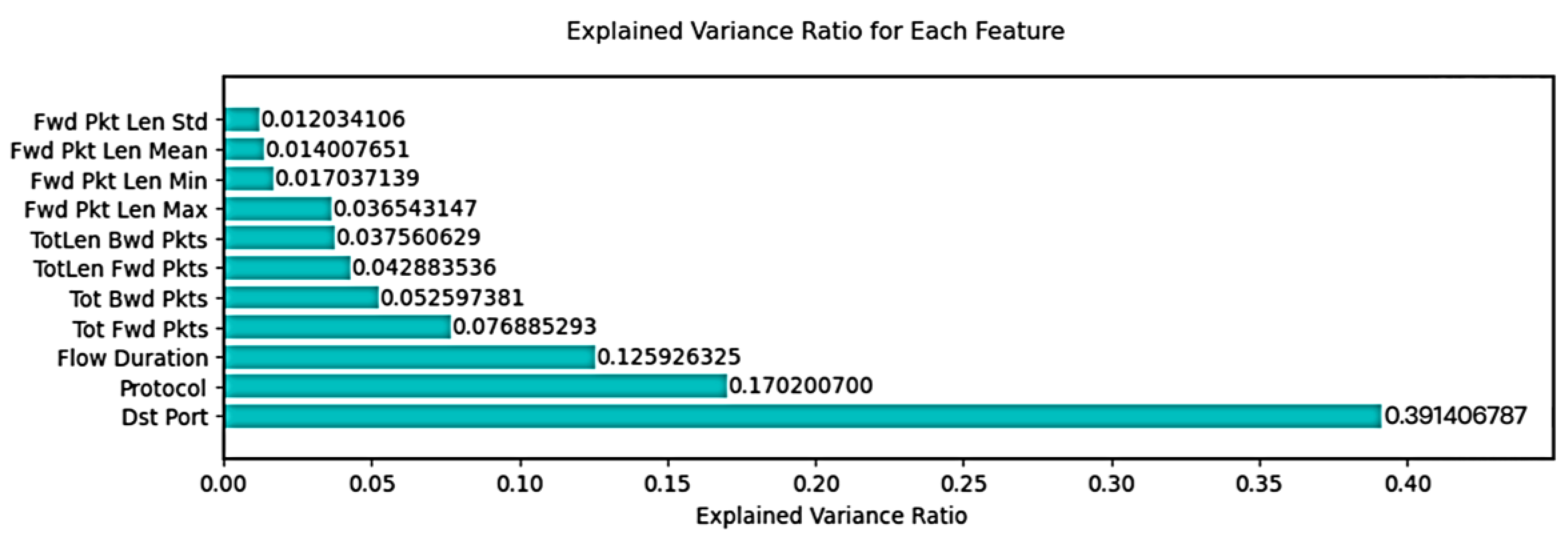
| Feature Name | Importance Score |
|---|---|
| Dst Port | 0.391406787 |
| Protocol | 0.170200700 |
| Flow Duration | 0.125926325 |
| Tot Fwd Pkts | 0.076885293 |
| Tot Bwd Pkts | 0.052597381 |
| TotLen Fwd Pkts | 0.042883536 |
| TotLen Bwd Pkts | 0.037560629 |
| Fwd Pkt Len Max | 0.036543147 |
| Fwd Pkt Len Min | 0.017037139 |
| Fwd Pkt Len Mean | 0.014007651 |
| Fwd Pkt Len Std | 0.012034106 |
| Study | Method | Feature Selection | CPU Time (s) | Accuracy | F1 Score | Precision | Recall | ROC | MCC | PCC/BA |
|---|---|---|---|---|---|---|---|---|---|---|
| S. Ullah. et al. [14] | DT Class Balance (SMOTE) | RF (30 features) | 0.18 (Train Time) | 0.9998 | n/a | n/a | n/a | n/a | n/a | n/a |
| M. A. Khan. [15] | HCRNNIDS | RF | 200–250 (Train Time) | 0.9775 | 0.976 | n/a | n/a | n/a | n/a | n/a |
| J. Kim. et al. [10] | CNN | Manual Feature Extraction | 300–900 (Train Time) | 0.960 | n/a | n/a | n/a | n/a | n/a | n/a |
| R. Qusyairi. et al. [3] | Ensemble Model | Chi-Square and Spearman’s Rank (23 Features) | n/a | 0.988 | 0.979 | n/a | n/a | n/a | n/a | n/a |
| S. Chimphlee. et al. [4] | MLP (Min–Max Normalization, Class Balance (SMOTE) | RF (16 Features) | n/a | n/a | 0.99462 | n/a | n/a | 0.99311 | 0.98151 | 0.99334 |
| Our Model 1 | XGBoost (Min–Max Normalization) | PCA (11 Features) | 50.09 (All Time) Train and Test Time | 0.997706 | 0.949388 | 0.920757 | 0.98879 | 0.993236 | 0.989180 | 0.98879 |
| Our Model 2 | XGBoost (Z-score Normalization) | PCA (11 Features) | 50.89 (All Time) Train and Test Time | 0.997698 | 0.949373 | 0.92074 | 0.988776 | 0.993227 | 0.989142 | 0.988776 |
Disclaimer/Publisher’s Note: The statements, opinions and data contained in all publications are solely those of the individual author(s) and contributor(s) and not of MDPI and/or the editor(s). MDPI and/or the editor(s) disclaim responsibility for any injury to people or property resulting from any ideas, methods, instructions or products referred to in the content. |
© 2023 by the authors. Licensee MDPI, Basel, Switzerland. This article is an open access article distributed under the terms and conditions of the Creative Commons Attribution (CC BY) license (https://creativecommons.org/licenses/by/4.0/).
Share and Cite
Songma, S.; Sathuphan, T.; Pamutha, T. Optimizing Intrusion Detection Systems in Three Phases on the CSE-CIC-IDS-2018 Dataset. Computers 2023, 12, 245. https://doi.org/10.3390/computers12120245
Songma S, Sathuphan T, Pamutha T. Optimizing Intrusion Detection Systems in Three Phases on the CSE-CIC-IDS-2018 Dataset. Computers. 2023; 12(12):245. https://doi.org/10.3390/computers12120245
Chicago/Turabian StyleSongma, Surasit, Theera Sathuphan, and Thanakorn Pamutha. 2023. "Optimizing Intrusion Detection Systems in Three Phases on the CSE-CIC-IDS-2018 Dataset" Computers 12, no. 12: 245. https://doi.org/10.3390/computers12120245
APA StyleSongma, S., Sathuphan, T., & Pamutha, T. (2023). Optimizing Intrusion Detection Systems in Three Phases on the CSE-CIC-IDS-2018 Dataset. Computers, 12(12), 245. https://doi.org/10.3390/computers12120245