The Fifteen Puzzle—A New Approach through Hybridizing Three Heuristics Methods

Hasan, Dler O.; Aladdin, Aso M.; Talabani, Hardi Sabah; Rashid, Tarik Ahmed; Mirjalili, Seyedali

doi:10.3390/computers12010011

Open AccessArticle

The Fifteen Puzzle—A New Approach through Hybridizing Three Heuristics Methods

¹

Department of Applied Computer, College of Medicals and Applied Sciences, Charmo University, Sulaymaniyah, Chamchamal 46023, Iraq

²

Department of Technical Information Systems Engineering, Erbil Technical Engineering College, Erbil Polytechnic University, Erbil 44001, Iraq

³

Computer Science and Engineering Department, University of Kurdistan Hewler, Erbil 44001, Iraq

⁴

School of Information and Communication Technology, Griffith University, Brisbane, QLD 4111, Australia

^*

Author to whom correspondence should be addressed.

Computers 2023, 12(1), 11; https://doi.org/10.3390/computers12010011

Submission received: 25 November 2022 / Revised: 24 December 2022 / Accepted: 27 December 2022 / Published: 3 January 2023

Download

Browse Figures

Review Reports Versions Notes

Abstract

:

The Fifteen Puzzle problem is one of the most classical problems that has captivated mathematics enthusiasts for centuries. This is mainly because of the huge size of the state space with approximately 10¹³ states that have to be explored, and several algorithms have been applied to solve the Fifteen Puzzle instances. In this paper, to manage this large state space, the bidirectional A* (BA*) search algorithm with three heuristics, such as Manhattan distance (MD), linear conflict (LC), and walking distance (WD), has been used to solve the Fifteen Puzzle problem. The three mentioned heuristics will be hybridized in a way that can dramatically reduce the number of states generated by the algorithm. Moreover, all these heuristics require only 25 KB of storage, but help the algorithm effectively reduce the number of generated states and expand fewer nodes. Our implementation of the BA* search can significantly reduce the space complexity, and guarantee either optimal or near-optimal solutions.

Keywords:

Fifteen Puzzle; heuristic search; inadmissible heuristic function; metaheuristic; bidirectional search; unidirectional search

1. Introduction

The Fifteen Puzzle is a standard sliding puzzle invented by Samuel Loyd in the 1870s [1] that consists of 15 tiles with one tile missing within a 4 × 4 grid. The fifteen tiles are numbered from 1 to 15. The numbered tiles should initially be ordered randomly. The aim of the game is to slide the tiles that are located next to the space into the space (one at a time) to achieve the numerical order of the tiles from left to right with the blank at the bottom right/top left corner in a minimum time and with minimum moves. Automatically solving the Fifteen Puzzle is very challenging because the state space for the Fifteen Puzzle contains about 16! /2≈10¹³ states [2]. The Fifteen Puzzle contains 16! instances but only half of the instances are solvable [3,4]. Optimal solutions for any solvable instances of the Fifteen Puzzle can take from 0 to 80 moves [5,6]. The two common heuristic search algorithms, A* [7] and iterative deepening A* (IDA*) [8], have been successfully used for computing optimal solutions for the Fifteen Puzzle instances. These algorithms are guided by heuristic functions, which are estimates of the number of moves required to solve any given puzzle configuration.

The most common heuristic functions that have been used to reduce the search space are misplaced tile (MT), MD, LC and pattern databases (PDBs) [9,10,11]. WD has also been used, but is not common. MT is the number of tiles that are not in their goal positions. MD is the sum of the distance of each tile from its goal position. LC is the sum of two moves for each pair of conflicting tiles that are in their goal row or column positions but in the wrong order. The WD was developed by [12], and counts the vertical moves and horizontal moves separately, while considering the tiles’ conflict with each other. PDBs are heuristics in the form of lookup tables. The two heuristics misplaced tile and Manhattan distance were used with the A* algorithm for optimally solving the Eight Puzzle problem by [13]. The Manhattan distance and linear conflict heuristics were combined and used with the IDA* algorithm for the Fifteen Puzzle by [14]. The walking distance heuristic was developed and used (with the IDA* search) by [12] for the Fifteen Puzzle. To the best of our knowledge, the walking distance heuristic has not been used in any research for the Fifteen Puzzle. The pattern database heuristics were first introduced by [15] and then used by many researchers, and now there are various types of pattern databases [16]. The main drawback of pattern databases is that they require a large amount of memory (several gigabytes for some types of pattern databases) [16,17]. Flener, Korf, and Hanan [18] claimed that an effective heuristic for the Fifteen Puzzle is the 7–8 additive pattern database, but this heuristic requires a lot of storage space and can be memory-intensive at about 575 megabytes.

All the heuristics used to estimate how close a state is to the goal suffer from a number of drawbacks. For example, some of them are not very accurate at estimating the remaining distance to a goal, such as MD, MT, and WD, and the others are accurate but require a lot of storage space, such as PDBs. The main objective of this paper is to combine some heuristics to accurately estimate the cost from the current state to the goal state without generating a lot of states or requiring a large amount of storage space to store the nodes. The contribution of this paper is to hybridize the three heuristics MD, LC, and WD to estimate the number of steps to the goal state. Moreover, to increase the effectiveness of the heuristic function, the MD value is divided by three. We use this heuristic in such a way to significantly reduce the number of generated nodes to solve the puzzle states. Using these heuristic algorithms in this way cannot be guaranteed to give an optimal solution, but they usually find an optimal solution or a solution that is one to six moves away from the optimum and, in some rare cases, more than six moves away from the optimum. For the most difficult states, we run two searches—a forward search from the initial state and a backward search from the end state (goal state), which is called a bidirectional search. This is for the sake of improving the algorithm performance.

This paper is structured as follows. Section 2 is devoted to presenting and discussing the implementation of our BA* algorithm. Section 3 presents and evaluates the three heuristics we use to solve the Fifteen Puzzle problem. Section 4 presents the efficient way of hybridizing the three heuristics for solving the Fifteen Puzzle. Section 5 presents and discusses the results and their comparisons. Section 5.1 compares our implementation of the BA* algorithm with the artificial bee colony (ABC) algorithm in terms of efficiency and inadmissibility. Section 5.2 discusses the comparison between bidirectional A* (BA*) search and unidirectional A* (UA*) search. Section 5.3 describes the experiments performed with our implementation of the BA* algorithm and also compares the results obtained by our algorithm with the results obtained by the IDA* algorithm with MD and LC heuristics. Finally, Section 6 highlights the main conclusion of this study.

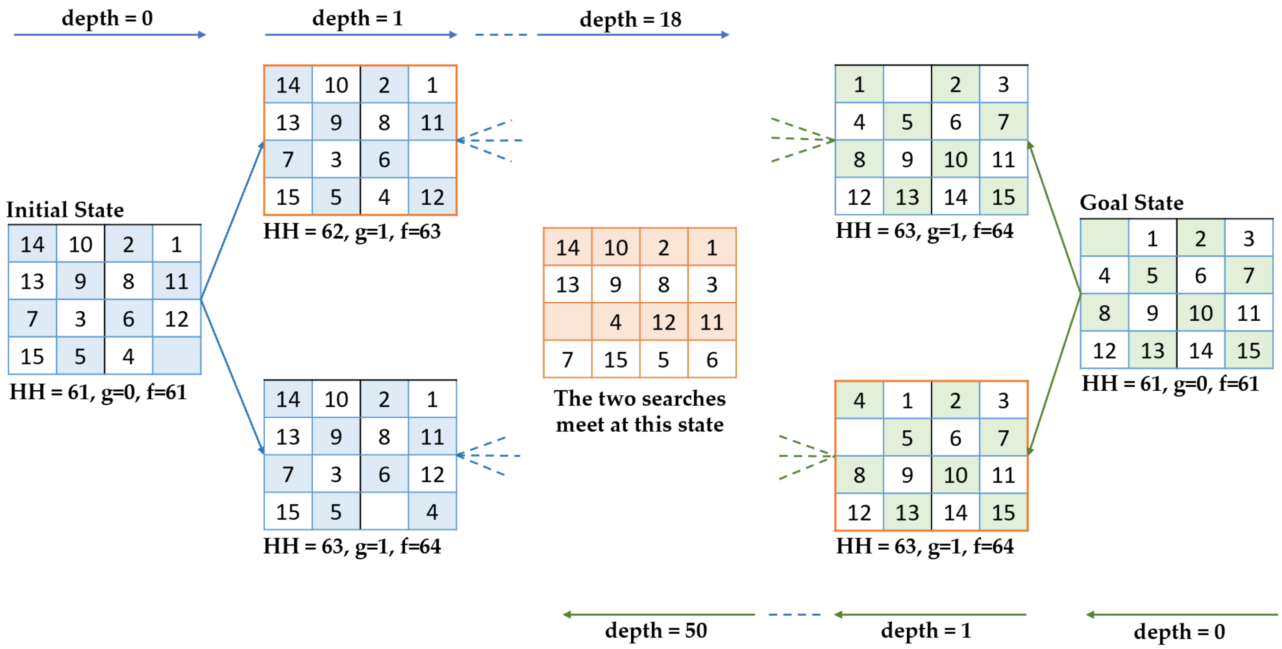
2. Bidirectional A* Algorithm

The IDA* and A* are the two most popular heuristic search algorithms widely used to solve the Fifteen Puzzle problem. The A* algorithm is one of most well-regarded algorithms in artificial intelligence for finding the shortest path or the smallest number of moves from the initial state to the goal [7]. Despite being complete, this algorithm has some disadvantages that can make it inefficient, especially for complex and large puzzle problems. This is because billions of nodes need to be expanded and generated for the difficult states, and in the A* algorithm all the generated nodes are kept in memory, which can lead to running out of memory, or sometimes finding a solution takes a long time. The IDA* algorithm is a variant of the A* algorithm that can be implemented for solving the Fifteen Puzzle [8]. Due to the fact that IDA* does not store the expanded nodes in memory, it uses less space and expands nodes faster than the A* algorithm. Even though the IDA* algorithm is more efficient than the A* algorithm, we still use the A* algorithm in this paper for several reasons. First of all, since we use bidirectional search, the A* algorithm is a good choice because it stores all the generated nodes in memory, and this leads to frontier intersections that can be easily tested [9]. Secondly, the A* algorithm with the heuristics that we use only generates a few states, and this does not cause the algorithm to run out of memory. Thirdly, since the A* algorithm retains the generated states in memory, each state is generated once.

Today, there are several variants of the A* algorithm since its performance can be varied depending on several methods. One of the optimization methods is bidirectional search, which is commonly used nowadays [19,20,21,22] since it can improve the efficiency of the algorithm in terms of space and time complexity. Another method is heuristic function, which directly affects the algorithm’s efficiency, and, therefore, there are several heuristics proposed for estimating the distances to remaining unexplored nodes [20]. Additionally, there are other variants of the A* algorithm in which the heuristic cost is weighted differently, and this has been utilized to speed up the A* algorithm [19,22]. This paper utilized all three mentioned methods to improve the A* algorithm’s efficiency.

Algorithm 1 gives the pseudocode for the bidirectional A* (BA*) algorithm. Some notations are used, such as OpenList, ClosedList, and NeighboringState, which denote the states that have been visited but not expanded, the states that have been visited and expanded, and the state that is directly connected to the current state. There are separate copies of these variables for both the forward and backward search, with a subscript (F or B) indicating the direction:

Forward search: OpenList_f, ClosedList_f, and NeighboringState_f, etc.

Backward search: OpenList_b, ClosedList_b, and NeighboringState_b, etc.

The BA* algorithm for each one of the two searches (forward and backward search) needs two lists: a closed list, which is used for storing all the puzzle states that have been visited and expanded, and an open list, which is used for storing the puzzle states that have been visited but not expanded. At each step, the heuristic value and the depth cost of the current state is determined. Then, the states inside the open list are sorted according to the heuristic values in increasing order. At every step, the head of the open list, which has the lowest evaluation function value (which is the heuristic value plus the path cost), is removed from the open list and then checked to see whether it is the goal state (start state for backward search) or not. If the head state is the goal state (start state for backward search), the algorithm reconstructs the path to the goal (to the start for backward search). If the head state is not the goal (is not the start for backward search), it is checked to see if it is in the closed list of the opposite search direction, and if it is there, the algorithm reconstructs the solution path from the two searches. When the goal (start for backward search) is not found, the head state is expanded (all the valid moves are specified) and it is placed on the closed list. Then, all the successors of the head state which are not already on the closed list are stored in the open list. As is shown in Algorithm 1, the forward search starts first and continues until 75,000 states are expanded, but after the first step of the cycle, the forward search continues until 15,000 states are expanded. If the solution path from the start state to the goal state is not found while generating this number of states, the forward search stops, and the backward search starts. The backward search continues until 75,000 states are expanded (until 15,000 states are expanded after the first step of the cycle). If, during that period, the solution path from the goal state to the start state is not found, the backward search stops, and the forward search starts again. This process will continue until the solution path is found.

Algorithm 1. BA* algorithm pseudocode

function BA* (StartState, GoalState)
Initialise:
Iterator_f to control the loop
OpenList_f to store the states to be traversed
ClosedList_f to store already traversed states
OpenList_b to store the states to be traversed
ClosedList_b to store already traversed states
if Iterator_f = 0 then
set depth cost of StartState (g(s) in Equation (2)) to zero
calculate HH value from StartState to GoalState. Equation (3)
calculate evaluation function for StartState. Equation (2)
add StartState into OpenList_f and ClosedList_f
while OpenList_f is not empty do
CurrentState_f is state with lowest evaluation function value (Equation (2)) in OpenList_f
remove CurrentState_f from OpenList_f
if CurrentState_f is GoalState then
reconstruct the solution path from StartState to CurrentState_f, and terminates the loop
for each NeighboringState_f of CurrentState_f do
if NeighboringState_f is not in ClosedList_f then
depth cost of NeighboringState_f is equal to the depth cost of CurrentState_f plus one
calculate HH value from NeighboringState_f to GoalState. Equation (3)
calculate evaluation function for NeighboringState_f. Equation (2)
add NeighboringState_f into ClosedList_f
add NeighboringState_f into OpenList_f
if NeighboringState_f is in ClosedList_b then
reconstruct the solution path from the two searches: from StartState to NeighboringState_f
and from NeighboringState_f to GoalState, and terminates the loop
increase Iterator_f by 1
if Iterator_f mod 15000 is equal to 0 after the first step of the cycle or Iterator_f mod 75000 is equal to 0 then
->Expand in the backward direction, analogously

To further explain Algorithm 1, Figure 1 illustrates how the two searches work. The puzzle state used in Figure 1 is Korf’s 15-puzzle problem instance #82 [8]. At the beginning, the first search (forward search) starts from the initial state and the evaluation function value (Equation (2)) for it is calculated, which is the summation of the heuristic value (Equation (3)) and the depth cost (g). After expanding the initial state, two new puzzle states are generated at depth one, the evaluation function value for each of them is calculated, and the state with the minimum evaluation function value is expanded (as shown in Figure 1, the state with the evaluation function value 63 is expanded). At each step, the puzzle state is checked to see whether it is the goal state or not or, or whether it is in the closed list of the opposite search direction. If the goal state is not found after expanding 75,000 states, the backward search starts from the goal state. The same process as the forward search is conducted. As illustrated in Figure 1, at depth 50, the backward search meets a puzzle state which was already generated by the forward search at depth 18. Then, the algorithm reconstructs the path from the two searches, which is 68 moves.

3. Heuristic Functions

A heuristic is an informed guess to choose the next node to visit when exploring a search space. A heuristic can lead the algorithm to a solution or fail to reach the goal. The three heuristics which are used in this paper are Manhattan distance, walking distance, and linear conflict. Figure 2 (a) shows an arbitrary start state of the Fifteen Puzzle and (b) shows the goal state of the Fifteen Puzzle. The tiles are denoted by t_i and the blank by t₀. The sequences are <t₁, t₄, t₂, t₃, t₁₃, t₆, t₇, t₈, t₅, t₁₀, t₁₁, t₀, t₉, t₁₄, t₁₅, t₁₂> for the start state and <t₁, t₂, t₃, t₄, t₅, t₆, t₇, t₈, t₉, t₁₀, t₁₁, t₁₂, t₁₃, t₁₄, t₁₅, t₀> for the goal state, as shown in Figure 2.

The Manhattan distance of a puzzle is the sum of the horizontal and vertical distance of each tile (except the blank tile) from its goal position [8]. For the initial state of the Fifteen Puzzle shown in Figure 2, only the tiles t₄, t₂, t₃, t₁₃, t₅, t_9, and t₁₂ are not in their goal positions, and they are away from their goal positions by 2, 1, 1, 2, 1, 1, and 1, respectively. Therefore, the heuristic function value is 9 (2 + 1 + 1 + 2 + 1 + 1 + 1). This means that the current state needs at least 9 moves to reach the goal. Manhattan distance is admissible because it never overestimates the number of moves to the goal and each tile must at least be moved from its current position to its goal position, and only vertical and horizontal movement is allowed. Therefore, the Manhattan distance value of any state is less than or equal to the number of moves that the state needs to reach the goal. The Manhattan distance of a tile in a puzzle can be found using Equation (1) (

s

is the current state) [17]:

h (s) = \sum_{i = 1}^{n} (|x_{i} (s) - \bar{x_{i}} |+| y_{i} (s) - \bar{y_{i}}|)

(1)

LC, which is used to enhance the effectiveness of the Manhattan distance, adds two additional moves to the Manhattan distance for each pair of conflicting tiles that would have to be swapped to reach the goal state. Two tiles, t_i and tj, are in a linear conflict if both tiles are positioned in their goal row or column but in the wrong order, or, in other words, they are reversed relative to their goal location [14]. For example, in Figure 2, the tile t₄ conflicts with tiles t₂ and t₃, and by changing the row of tile t₄ we can eliminate these conflicts. The tile t₁₃ conflicts with tiles t₅ and t₉ because they are in the correct column but inverse order. In this case, t₉ must move one place to the right to let the others pass by and then move back to its column position. These four moves are not counted in the Manhattan distance. Therefore, two additional moves are added to the Manhattan distance for each pair of conflicting tiles and the heuristic evaluation function remains admissible.

So far, the total cost function for the initial state in Figure 2 is equal to 13 (9 for the Manhattan distance, 4 for the linear conflict), while the optimal solution for the initial state is 29 moves. Therefore, using these two heuristics cannot make the algorithm efficient, especially for complex and large puzzle problems, and finding the solution takes a long time. This is because Manhattan distance does not capture the conflicts and interactions between the tiles, and this leads to heavily underestimating the actual optimal solution cost in almost all the problem instances of the Fifteen Puzzle [23], and linear conflict only adds two moves for every two tiles which are positioned in the correct row/column but inverted. Walking distance counts the vertical moves and horizontal moves separately while considering the tiles’ conflict with each other [12]. According to the goal state in Figure 2, all four tiles (t₁, t₄, t₂, and t₃) in the first row of the initial state are from the first row of the goal state and no tiles are from the other rows of the goal state. The same approach is used for the other rows, as is shown in Table 1.

To calculate the horizontal walking distance, we can only swap the blank tile with any single tile from the row above or below, and the order of the tiles in each row is irrelevant. We keep swapping until all the tiles are in their goal rows. The minimum number of moves needed to take all the tiles to their goal row positions is the horizontal walking distance. We can apply the same procedure to calculate the vertical walking distance by taking all the tiles to their goal column positions with the minimum number of moves, and each tile can only be taken into a column adjacent to the column containing the blank tile and swap places with it. The order of the tiles in each column is irrelevant. The total walking distance is the sum of the number of horizontal and vertical moves. To further explain Table 1, Figure 3 illustrates how WD can be calculated manually step by step for the initial state in Figure 2. Two 4 × 4 tables are needed, one for computing the horizontal WD value and another one for computing the vertical WD value.

The table of the horizontal WD in Figure 3 has four ‘A’ elements in the first row, which means that all the tiles t₁, t₄, t₂, and t₃ are from the first row of the goal state. It has one ‘D’ element and three ‘B’ elements in the second row, which is because t₁₃ is from the fourth row of the goal, and t₆, t₇, and t₈ are from the second row of the goal. It has one ‘B’ element and two ‘C’ elements with a blank (t₀) element in the third row, which is because t₅ is from the second row of the goal, and t₁₀ and t₁₁ are from the third row of the goal. It has two ‘C’ elements and two ‘D’ elements in the fourth row, which is because t₉ and t₁₂ are from the third row of the goal, and t₁₄ and t₁₅ are from the fourth row of the goal. As is shown in Figure 3, only five steps are needed to take all the tiles to their goal row position, which is the horizontal WD value for the initial state in Figure 2. The same procedure is used for building the table of the vertical WD and calculating the vertical WD value, except that when we build the table of vertical WD, we must specify which column each tile’s goal position is in. As can be seen in Figure 3, to take all the tiles to their column position, six steps are needed, which is the vertical WD value for the initial state in Figure 2. The total walking distance is the sum of the number of horizontal and vertical moves, which is 11 steps.

Since walking distance cannot be easily computed at runtime, we can precompute all these values and store them in the database, because if we do not precompute them, this heuristic can slow the search down significantly. Instead of fully calculating the walking distance during the search, a breadth-first search (BFS) can be executed backward from the goal state to obtain all the distinct tables for all the Fifteen Puzzle configurations (all possible configurations of the tiles), which are only 24,964 patterns, and store them in the database to speed up the search. The size of the database is relatively small at about 25 KB. The same database is used for calculating the number of horizontal and vertical moves. The maximum walking distance value is 70 (such as t₀, t₁₅, t₁₄, t₁₃, t₁₂, t₁₁, t₁₀, t₉, t₈, t₇, t₆, t₅, t₄, t₃, t₂, t₁), with 35 moves each for horizontal and vertical moves. WD is more accurate and efficient than Manhattan distance because the WD value is always greater than the MD value, as is illustrated in Figure 4.

Figure 4 shows the MD, WD, and optimal values for Korf’s 100 instances [8] after sorting the instances by optimal value. In all of them, the WD value is greater than the MD value, and Table 2 shows that the total WD value for all the 100 instances is greater than the total MD value. Table 2 also shows the minimal total cost (optimal solution) and total LC values for all the 100 instances.

The walking distance can also be enhanced by the linear conflict, because WD does not count the two moves which are determined by linear conflict for each pair of conflicting tiles. As shown in Figure 3, when calculating the horizontal or vertical WD values when we have two tiles in linear conflict, the first tile can slide to the row above or below, if that row contains a blank, without moving the second tile, and for the second tile this is also correct. For example, Figure 5 zooms in and shows a part of Figure 3 where the tile t₁₃ (D) that conflicts with the tile t₅ (B) can slide to the third row without moving the tile t₅ (B).

We have built the walking distance lookup table for both goal states with a blank at the bottom right and top left corner because the two different goal states have been used in many types of research and we also use these two different goal states in this paper.

4. Hybridized Heuristic Functions

Since we have no perfect heuristic function (exact distance function) to give us the exact number of moves needed to solve all the Fifteen Puzzle instances and each heuristic has its way to calculate the distance between the current state to the goal state, it is desirable to combine multiple heuristics which can complete each other to estimate the solution cost. Combining several heuristics is generally the best way to more accurately estimate the cost of reaching the goal, but it is challenging [24,25,26]. Multiple heuristics have been used in different ways. The most common way to use multiple heuristics is to combine different heuristics and use their maximum value. Holte et al. [16] showed that taking the maximum heuristic value from several heuristics can lead to reduced node generation and result in improved performance of the search. When two or more admissible heuristics are combined, taking their maximum, that is, by defining (

hmax (s) = \max (h 1 (s), h 2 (s))

. ), is also admissible [16,27].

Another way to use multiple heuristics is cost partitioning or cost splitting, which has been used by many researchers [28,29,30] and is a technique to add multiple heuristic values in an admissible way with operator cost partitioning by distributing the cost of each operator among them. This technique has a drawback in finding good cost partitioning [29]. Korf and Taylor [31] took advantage of several heuristics including Manhattan distance, linear conflict, last moves, and corner tile to improve the accuracy of the heuristic evaluation function and result in improved search performance of the IDA* search. In addition, they used the heuristics in a way that keeps the them admissible; for example, when the same tile is involved in a corner tile and linear conflict, the extra moves are added only once. Therefore, whenever we combine multiple heuristics and we want to find the optimal solution, we must be sure that the actual distance for any tile is not calculated more than once. Those heuristics are not complex, and it is easy to check which tiles are involved in multiple heuristics. Manhattan distance and walking distance, the two heuristics that we use in this paper, are complex and it is not easy to check which tiles’ actual distance to their goal position is counted by the two heuristics.

Each heuristic has its strengths and weaknesses. Therefore, we must determine the weaknesses and strengths of the heuristics when we want to combine multiple to create a more accurate heuristic function. The main drawback of Manhattan distance is measuring each tile’s distance to its goal position without considering the interference from any other tiles [18]. For example, according to the MD, the tiles t₆, t₇, t₈, t₁₀, t₁₁, t₁₄, and t₁₅ in the initial state shown in Figure 3 need zero moves to reach their goal positions since they are already in them. This estimation is not correct because it is not possible to take the tiles t₄, t₂, t₃ t₁₃, t₅, and t₉ to their goal positions without moving some of the tiles t₆, t₇, t₈, t₁₀, t₁₁, t₁₄, and t₁₅. On the other hand, WD considers interactions between tiles and it calculates the distance of the tiles to their goal positions like MD. As illustrated in Figure 6, which is a part of Figure 3, one of the tiles t₇, t₁₁, and t₁₅ makes two moves while calculating the WD value, which proves that WD is more efficient than MD.

WD is not exactly equal to MD plus the interference of tiles with each other. It seems that the WD heuristic considers interactions between tiles and the distance of each tile to its goal position, but we think it finds the interaction of tiles to be more significant than their distances to their end positions, because there are many Fifteen Puzzle problem instances that have the same MD and WD values. For instance, 23 out of Korf’s 100 instances have the same WD and MD values despite a lot of interactions between their tiles. Additionally, for the instance <t₁₅, t₄, t₇, t₁₁, t₅, t₈, t₀, t₃, t₁₄, t₂, t₁₂, t₁₃, t₁, t₆, t₁₀, t₉>, the WD and MD are both 35 even though there are a lot of interactions between the tiles. If the WD is equal to the exact MD plus the conflicts between the tiles, the WD value for that Fifteen Puzzle instance must be greater than the MD value, not equal to it. Therefore, this proves that the WD is not equal to the exact MD plus the conflicts between the tiles for the Fifteen Puzzle problem instances. In spite of this, WD works somewhat similarly to but not exactly the same as MD, since WD takes each tile to its goal column–row position when calculating the horizontal and vertical values for a puzzle instance, as is illustrated in Figure 3. In general, WD is more efficient and better than MD because WD is never less than MD, as is illustrated in Figure 4. Because of this, we use WD and LC as the main heuristics together with MD as a helping heuristic to assist the main heuristics. Since we use MD as a helping heuristic, the MD value is divided by 3. In this way, the MD value is reduced to a number when it is added to the main heuristics values, so the result will be close to the optimal solution length.

As explained before, WD mainly considers the interactions between the tiles, and it calculates the distance of the tiles to their actual positions in a way similar to MD. Therefore, to compensate, the calculating tiles’ distance to their goal position MD is used but not the whole MD value. The MD value is divided by a number (which is three) so that the summation of WD, LC and MD/3 will be close to the optimal solution length. For example, if we sum the total WD value (3957), LC value (212), and MD value divided by three (3705/3), as is shown in Table 2, the result will be 5404, and this result is near to the total optimal solution value 5307 for Korf’s standard 100 random Fifteen Puzzle instances. Furthermore, this total overestimation is very small and it does not have a great impact on the results of BA* with HH, as the implementation of our algorithm finds an optimal solution or a solution that is near to the optimum and to reach the goal for each instance, a small number of states are generated. Because of this, we calculate the heuristic function in the evaluation function (Equation (2) [1]), as shown in Equation (3), named hybridizing heuristic (HH). To find the shortest path, the A* algorithm uses the evaluation function as it is shown in Equation (2), which is equal to the

g (s)

, the depth cost from the start state to the current state, plus the

h (s)

, the heuristic that estimates the distance from the current state to the goal state. The A* algorithm guarantees the optimal solution if the heuristic function is admissible.

f (s) = g (s) + h (s)

(2)

h (s) = \frac{m d (s)}{3} + w d (s) + l c (s)

(3)

5. Results and Discussions

In this section, to evaluate the efficiency and performance of our implementation of the BA* algorithm, we make some comparisons. Firstly, BA* with HH is compared with the ABC algorithm in terms of admissibility. Secondly, in terms of directionality, BA* and UA* are compared to show that the bidirectional search is more efficient than the unidirectional search, especially when there is a guarantee that the two bidirectional searches do not pass by each other without intersecting. Finally, the BA* search with HH is run on Korf’s 100 instances, along with a comparison with the IDA* search.

5.1. Inadmissible Heuristics

An algorithm can guarantee finding the shortest path or the smallest number of moves from the initial state to the goal only if the heuristic function never overestimates the actual path cost from the current state to the goal state, which we call an admissible heuristic [32]. Due to the reason that finding the optimal solution for the Fifteen Puzzle is too expensive and requires searching through a very large number of paths and generating a large number of nodes [33], many types of research have been conducted to obtain near-optimal solutions instead of exact optimal solutions [34,35]. Thayer, Dionne, and Ruml [36] state that, to reduce the solving time, a near-optimal solution is a practical alternative. To reduce the number of generated nodes, we incorporated aspects from the three heuristics to create a better one and the heuristic function in the evaluation function (Equation (2) [1]) is calculated as shown in Equation (3). As shown in Equation (3), three heuristics are combined to estimate the cost from a given state (node) to the goal state. The value of the Manhattan distance is divided by three because calculating in that way leads to fewer nodes to be generated during the search. Because of the previous reasons, the algorithm heuristic cannot guarantee finding the goal with the smallest number of moves, but this brings some advantages. Firstly, a lesser number of nodes are generated and it can very quickly find the goal. Secondly, the result is very close to the optimal solution. Since a bidirectional search has been used to find the path from the initial state to the goal state, the three heuristics have been used in both directions (search).

However, our implementation of the BA* algorithm with the three heuristics does not find optimal solutions for most of the Fifteen Puzzle instances; the difference between the solution length found by BA* and the optimal solution for each puzzle instance does not increase when the puzzle instance requires more moves to optimally reach the goal. Nowadays, metaheuristic optimization algorithms are widely used for solving complex problems [37,38,39]. One of the algorithms that has recently been used to obtain non-optimal solutions to the Fifteen Puzzle problems is a metaheuristic algorithm: artificial bee colony (ABC) [40]. Here, the BA* algorithm with HH is compared with the ABC algorithm to show that the obtained results of BA* are sufficiently accurate and much nearer to the optimal results. To increase the effectiveness and performance of the heuristic function of the ABC algorithm, three heuristics, PDB, MD, and LC, were combined. The ABC algorithm was run on 25 randomly generated solvable instances of the Fifteen Puzzle, but the algorithm did not produce an optimal solution for any of them; it provided solutions that are far from the optimum [40]. Tuncer [40] argued that the results produced by the ABC algorithm are acceptable even though the solution lengths are far from the optimal solution lengths. Furthermore, the difference between the solution costs obtained by the ABC algorithm and the optimal solutions for most of the puzzle instances increases when the puzzle instances require more moves to optimally reach the goal. For example, according to Table 3, the solution cost obtained by the ABC algorithm for the first nine puzzle instances that need fewer steps to optimally reach the goal is near to the optima, while the rest of the puzzle instances are very far from the optima. This is because these instances need more steps to optimally reach the goal. According to this example, the difference between the number of moves obtained by the ABC algorithm and the optimal solution will be big, especially for those states that require 80 moves to reach the goal. On the other hand, an important point about our implementation of the BA* algorithm is that the solution lengths for almost all the Fifteen Puzzle instances are zero to six moves away from the optimal solution lengths, even for the difficult states, as is shown in Table 3 and Table 4.

The BA* algorithm with HH was run on the same 25 initial states, and the results obtained by the BA* algorithm are very near to the optimal solutions compared to the results obtained by the ABC algorithm. For example, Table 3 shows that the average number of moves in the solutions that are obtained by the ABC algorithm is 58.76, while the average number of moves in the solutions that are obtained by the BA* algorithm is 50.4. In addition, the average number of moves in the solutions found by BA* is only 1.92 away from the average cost of the optimum solution, which is 48.48, while the average number of moves in the solutions found by ABC is 10.28 away from the average cost of the optimum solution. Figure 7 illustrates the results of the 25 states presented in Table 3 obtained by the ABC and BA* algorithm.

Table 3. Comparison of results between BA* algorithm and ABC algorithm.

NO	INITIAL STATE	Optimal LEN	LEN (ABC) BEST	LEN (BA*)
1	1 5 2 7 10 14 11 6 15 12 9 3 13 0 8 4	34	37	34
2	5 6 10 7 1 3 11 8 13 4 15 9 14 0 2 12	38	43	38
3	1 11 6 2 10 13 15 5 3 12 0 4 9 7 14 8	40	46	42
4	6 5 2 7 13 0 10 12 4 1 3 14 9 11 15 8	44	49	46
5	4 3 10 7 6 0 1 2 12 15 5 14 9 13 8 11	44	52	46
6	4 10 3 2 1 0 7 8 9 6 13 15 14 12 11 5	44	51	52
7	3 4 11 2 9 1 14 15 7 6 0 8 5 13 12 10	44	51	44
8	3 10 2 5 15 6 13 4 0 11 1 7 9 12 8 14	46	52	48
9	9 4 0 3 14 7 5 12 15 2 13 6 10 1 8 11	46	54	48
10	7 1 12 10 6 11 15 4 0 2 5 14 3 13 8 9	48	59	50
11	1 13 5 7 14 9 10 12 11 8 2 15 6 0 4 3	48	62	50
12	13 9 5 12 10 2 4 11 3 8 0 7 1 14 6 15	48	64	50
13	2 13 6 1 14 5 11 0 12 4 8 10 9 3 15 7	50	66	50
14	11 3 12 9 2 8 10 14 0 7 15 13 1 6 5 4	50	68	52
15	7 6 15 12 14 1 13 3 0 9 8 4 2 11 5 10	50	68	52
16	5 8 13 15 14 0 1 7 4 6 10 2 11 9 12 3	52	59	56
17	12 2 5 11 10 0 1 6 3 14 8 9 7 4 13 15	52	62	52
18	13 3 2 8 12 0 5 1 11 6 9 15 4 14 7 10	52	63	52
19	7 13 1 4 9 12 8 5 15 14 0 6 11 2 3 10	52	59	52
20	8 11 12 10 2 0 15 1 14 6 4 3 7 9 5 13	54	61	58
21	6 8 12 13 7 2 5 14 9 3 1 15 11 0 10 4	54	65	54
22	9 12 2 5 11 1 10 14 0 4 3 8 6 15 7 13	54	67	60
23	10 12 11 7 8 9 14 5 3 13 4 1 6 0 2 15	56	69	56
24	3 10 14 5 1 12 11 8 15 7 9 6 2 0 13 4	56	71	58
25	9 3 12 5 4 14 6 11 8 7 15 13 10 0 2 1	56	71	60
Average		48.48	58.76	50.4

5.2. Bidirectional and Unidirectional Search

In a bidirectional search, two separate searches are sequentially or simultaneously run. One search, called the forward search, is normal, starting from the initial state and moving toward the goal state, and the other search, called the backward search, starts from the goal state and moves toward the initial state. The search process terminates once the two searches meet at a common node in the middle and the algorithm constructs a single path that extends from the initial state to the goal state [41,42,43,44]. Pohl [42] was the first person who introduced and implemented a bidirectional heuristic search algorithm with the name bidirectional heuristic path algorithm (BHPA) and he showed that a bidirectional search is more efficient than a unidirectional search. BHPA did not work as expected, since after the search frontiers meet, both directions of searches pass through the opposing frontier to ensure optimality of the solution, and this leads to the same node being expanded by the two searches. To resolve this issue, Kwa [45] created a bidirectional staged BS* heuristic search algorithm, which is derived from Pohl’s BHPA algorithm, to avoid the re-expansion of a state that has already been expanded in the opposite search. These days, there are several types of research that prove that a bidirectional search is very efficient at solving various problems [46,47,48,49,50].

As shown in Algorithm 1, we implemented a bidirectional search as follows: two sequential processes are run, one branching from the start state, the other branching from the goal state. The first search, “forward search”, starts from the initial state and will continue until 75,000 nodes are expanded. If the goal state is not reached, the second search, “backward search”, is initiated from the goal state towards the initial state and this search will continue until it expands 75,000 nodes. If the goal is not found, the backward search stops, and the forward search is performed again. The search process will continue to cycle until both directions meet or the solution is found. During the search, whenever a state is generated by one of the two searches, the algorithm checks if the state has already been generated by the opposite search, and, if it has, it reconstructs a solution path from the two searches. Korf and Schultze [51] were able to compute the number of unique states at each depth of the Fifteen Puzzle. According to [51], the number of generated nodes at each depth gradually increases from depth 0 to depth 53, then the number of generated nodes at each depth starts to gradually decrease from depth 54 to 80. Based on this, the bidirectional search may not be very effective, because the number of generated nodes at depth 53 decreases in both directions and it can be difficult for both searches to meet in the middle. Therefore, one of the problems for the bidirectional search is that the two searches may not meet or may pass by each other without intersecting, but the A* algorithm retains all the visited nodes in the memory, which ensures that the two searches meet and frontier intersections can be easily tested [9]. Furthermore, there can be more than one optimal solution or non-optimal solution for the Fifteen Puzzle instances that can help the two searches not pass by each other without intersecting [52]. Additionally, the bidirectional search is very useful when the problem has not had many goals.

Our implementation of the BA* search can reduce the number of generated states because we use a priority queue to store the estimated costs of states (nodes), and the state from anywhere in the entire queue (not at a specific level) with the lowest evaluation function value (the heuristic value plus the path cost) is always selected to expand. Therefore, the algorithm visits the states in order of their costs, not level by level, which results in speeding up the search. Our implementation of the BA* search can find optimal or near-optimal solutions to even the difficult states and with a small fraction of states expanded (and stored) compared to the unidirectional A* (UA*) search. Table 4 shows that the bidirectional search is more efficient than the unidirectional search concerning generated nodes. In Table 4, we run the BA* and UA* search on 28 different states that require 80 moves. The goal state with a blank tile in the top left corner is used for the first 11 instances, but the goal state with a blank tile in the bottom right corner is used for the remaining 17 instances. The first nine instances were presented by [53], instances 10 and 11 were presented by [54], and the last 17 states were found by [55]. According to Table 4, the BA* search is more efficient than the UA* search in terms of node expansion, and, for seven of the states, UA* is unable to find a solution path and it runs out of memory before finding a solution. Even though the average solution cost obtained by UA* is less than the average solution cost obtained by BA*, the difference is not significant; it is only 2.3. Additionally, the average number of states generated by the BA* search is significantly less than those generated by the UA* search, even though the number of states generated by the UA* search for seven states has not been counted due to running out of memory.

Table 4. Comparison of BA* search and UA* search for the 28 difficult Fifteen Puzzle instances requiring 80 moves.

NO	INITIAL STATE	Optimal LEN	LEN (UA*)	Generated States (UA*)	LEN (BA*)	Generated States (BA*)
1	15 14 8 12 10 11 9 13 2 6 5 1 3 7 4 0	80	Memory ran out		88	187,592
2	15 11 13 12 14 10 8 9 7 2 5 1 3 6 4 0	80	84	138,505	84	138,505
3	15 11 13 12 14 10 8 9 2 6 5 1 3 7 4 0	80	82	1,605,359	86	367,391
4	15 11 9 12 14 10 13 8 6 7 5 1 3 2 4 0	80	82	771,924	86	420,441
5	15 11 9 12 14 10 13 8 2 6 5 1 3 7 4 0	80	84	1,207,604	86	199,905
6	15 11 8 12 14 10 13 9 2 7 5 1 3 6 4 0	80	82	809,360	82	185,126
7	15 11 9 12 14 10 8 13 6 2 5 1 3 7 4 0	80	Memory ran out		86	219,470
8	15 11 8 12 14 10 9 13 2 6 5 1 3 7 4 0	80	84	2,565,243	86	200,926
9	15 11 8 12 14 10 9 13 2 6 4 5 3 7 1 0	80	84	751,072	84	190,731
10	15 14 13 12 10 11 8 9 2 6 5 1 3 7 4 0	80	82	1,137,335	84	205,344
11	15 11 13 12 14 10 9 5 2 6 8 1 3 7 4 0	80	82	1,933,020	86	530,773
12	0 12 9 13 15 11 10 14 3 7 2 5 4 8 6 1	80	Memory ran out		88	186,644
13	0 12 10 13 15 11 14 9 3 7 2 5 4 8 6 1	80	84	2,096,287	84	207,896
14	0 11 9 13 12 15 10 14 3 7 6 2 4 8 5 1	80	84	949,297	84	198656
15	0 15 9 13 11 12 10 14 3 7 6 2 4 8 5 1	80	84	734,711	84	167,455
16	0 12 9 13 15 11 10 14 3 7 6 2 4 8 5 1	80	Memory ran out		86	256,899
17	0 12 14 13 15 11 9 10 3 7 6 2 4 8 5 1	80	84	917,307	86	205,555
18	0 12 10 13 15 11 14 9 3 7 6 2 4 8 5 1	80	82	1,623,362	86	341,405
19	0 12 11 13 15 14 10 9 3 7 6 2 4 8 5 1	80	Memory ran out		86	520,393
20	0 12 10 13 15 11 9 14 7 3 6 2 4 8 5 1	80	82	764,029	82	199,908
21	0 12 9 13 15 11 14 10 3 8 6 2 4 7 5 1	80	Memory ran out		86	213,147
22	0 12 9 13 15 11 10 14 8 3 6 2 4 7 5 1	80	84	998,668	86	205,473
23	0 12 14 13 15 11 9 10 8 3 6 2 4 7 5 1	80	84	1,372,770	86	416,315
24	0 12 9 13 15 11 10 14 7 8 6 2 4 3 5 1	80	82	1,205,808	86	213,283
25	0 12 10 13 15 11 14 9 7 8 6 2 4 3 5 1	80	84	105,242	84	105,242
26	0 12 9 13 15 8 10 14 11 7 6 2 4 3 5 1	80	82	2,259,670	86	534,581
27	0 12 9 13 15 11 10 14 3 7 5 6 4 8 2 1	80	Memory ran out		88	160,899
28	0 12 9 13 15 11 10 14 7 8 5 6 4 3 2 1	80	84	2,358,160	84	209,711
	Average	80	83.1	1,252,606	85.4	256,774

Table 5 [9] shows the comparison between the two searches, UA* and BA* with HH, which were implemented in this paper. According to Table 5, the space and time complexity of the UA* algorithm is

O (b^{d})

, where

b

is the branching and

d

is the depth of solution, whereas the space and time complexity of the BA* algorithm is

O (b^{d / 2})

, since two searches are run in the BA* algorithm; thus, the solution depth is divided by two. One significant point to notice is that the time and space complexity of the A* algorithm strongly depends on the heuristics, which heuristics are used, and how they are implemented [9]. Therefore, in this paper, we took advantage of the bidirectional search, the heuristics, and the way of implementing them (as shown in Equation (3)) to reduce the space complexity. Table 5 also presents the completeness and optimality of UA* and BA* with HH. It shows that both the searches are complete but not optimal. This is because of the way of using heuristics, as we mentioned before that BA* with HH guarantees either an optimal or near-optimal solution.

5.3. Experiments

In the study, the BA* algorithm was applied by combining the advantages of WD, LC, and MD heuristics. The algorithm was run on the 100 random initial states presented by [8], which is mainly to show the efficiency and performance of our implementation of BA*. In Korf’s goal state, the blank is located at the top left corner, and Korf used the IDA* search algorithm with the MD heuristic. Then, those 100 random initial states were used by [14], but this time the IDA* algorithm with MD and LC heuristics was run on them, and the result has been added to Table 6. Even though the implementation of the IDA* algorithm with MD and LC heuristics is quite old, we still compare our results with its results because we also use both MD and LC heuristics, albeit in different ways and with another heuristic (WD). Furthermore, our algorithm considerably reduces the number of generated nodes compared to the results of IDA* with the two heuristics MD and LC.

Table 6 shows that the number of states examined using BA* with HH is much less than the number of states examined using IDA* with MD and LC. For example, the average cost of states examined using IDA* with MD and LC is 37,596,318 states, while the average cost of states generated by BA* with HH is only 48,420 states. Furthermore, Table 6 also shows that the average solution cost that is obtained by BA* with HH is about 55.01, and this is very near the average optimal solution cost which is about 53.1 moves. In addition, the number of moves and the number of generated states in the solution of each instance using both the IDA* and BA* algorithms are also shown in Table 6. Moreover, it is evident in Table 6 that the solution length of 98% of the instances from zero to six moves is far from their optimal solution lengths.

Table 6 also demonstrates the number of state expansions and the WD, MD, and LC values for each of the puzzle instances. Figure 8 graphically shows the total number of states according to the cost difference between their optimal solutions and the solutions achieved by BA* with HH based on Table 6. Table 6 also shows that the solution of 39 states is zero moves away from optimum (they are optimal solutions), the solution of 36 states is two moves away from optimum, the solution of 17 states is four moves away from optimum, and the solution of six states are six moves away from optimum. The figure also shows that the solution of only one state is eight moves away from optimum and the solution of only one state is 10 moves away from optimum. Table 6 also presents the HH value for each instance and it shows that the HH value is very near to the instance’s optimal length. The average HH value is 54.04, only 0.97 away from the average optimal length, which is 53.07. The last column of Table 6 indicates the time (in seconds) it takes to solve each puzzle instance by BA* with HH.

In short, the most important thing about our implementation of BA* with HH is that it drastically reduces the search space without consuming a lot of storage space, since for all three heuristics used in this paper, only 25 KB is required. Furthermore, the results for each instance are very close to the shortest path length, even for complex puzzle states. Additionally, the estimation of HH for each instance shown Table 6 is near to the optimal length.

Table 6. Comparison of IDA* algorithm with MD and LC and BA* algorithm with HH for Korf’s 100 instances.

NO	INITIAL STATE	Optimal LEN	IDA* with MD + LC (Generated States)	BA* with HH (Generated States)	LEN (BA*)	BA* with HH (State Expansion)	WD	MD	LC	HH Value	Time (s) (BA*)
1	14 13 15 7 11 12 9 5 6 0 2 1 4 8 10 3	57	12,205,623	4348	59	2146	43	41	2	59	0.15
2	13 5 4 10 9 12 8 14 2 3 7 1 0 15 11 6	55	4,556,067	104,760	59	50,143	45	43	0	59	1.16
3	14 7 8 2 13 11 10 4 9 12 5 0 3 6 1 15	59	156,590,306	39,851	59	18,672	43	41	0	57	0.59
4	5 12 10 7 15 11 14 0 8 2 1 13 3 4 9 6	56	9,052,179	128,358	58	62,894	44	42	0	58	1.22
5	4 7 14 13 10 3 9 12 11 5 6 15 1 2 8 0	56	2,677,666	20,413	58	9635	44	42	2	60	0.41
6	14 7 1 9 12 3 6 15 8 11 2 5 10 0 4 13	52	4,151,682	4682	54	2234	40	36	4	56	0.15
7	2 11 15 5 13 4 6 7 12 8 10 1 9 3 14 0	52	97,264,710	150,410	54	75,251	34	30	0	44	1.57
8	12 11 15 3 8 0 4 2 6 13 9 5 14 1 10 7	50	3,769,804	22,921	54	11,354	36	32	4	51	0.43
9	3 14 9 11 5 4 8 2 13 12 6 7 10 1 15 0	46	88,588	1811	48	871	34	32	4	49	0.10
10	13 11 8 9 0 15 7 10 4 3 6 14 5 12 2 1	59	48,531,591	42,218	59	20,030	47	43	2	63	0.60
11	5 9 13 14 6 3 7 12 10 8 4 0 15 2 11 1	57	25,537,948	67,872	59	32,265	45	43	2	61	0.86
12	14 1 9 6 4 8 12 5 7 2 3 0 10 11 13 15	45	179,628	633	45	298	37	35	0	49	0.05
13	3 6 5 2 10 0 15 14 1 4 13 12 9 8 11 7	46	1,051,213	14,327	48	7164	36	36	2	50	0.34
14	7 6 8 1 11 5 14 10 3 4 9 13 15 2 0 12	59	53,050,799	153,470	63	76,125	43	41	2	59	1.47
15	13 11 4 12 1 8 9 15 6 5 14 2 7 3 10 0	62	130,071,656	43,608	64	20,685	46	44	2	63	0.54
16	1 3 2 5 10 9 15 6 8 14 13 11 12 4 7 0	44	2,421,878	67,984	44	34,375	24	24	2	34	0.86
17	15 14 0 4 11 1 6 13 7 5 8 9 3 2 10 12	66	100,843,886	206,372	76	98,417	54	46	0	69	2.38
18	6 0 14 12 1 15 9 10 11 4 7 2 8 3 5 13	55	5,224,645	19,272	57	9121	43	43	0	57	0.38
19	7 11 8 3 14 0 6 15 1 4 13 9 5 12 2 10	46	385,369	5381	46	2475	36	36	2	50	0.18
20	6 12 11 3 13 7 9 15 2 14 8 10 4 1 5 0	52	3,642,638	32,036	54	15,414	36	36	0	48	0.51
21	12 8 14 6 11 4 7 0 5 1 10 15 3 13 9 2	54	43,980,448	59,920	56	28,403	40	34	2	53	0.91
22	14 3 9 1 15 8 4 5 11 7 10 13 0 2 12 6	59	79,549,136	4517	63	2112	45	41	4	63	0.14
23	10 9 3 11 0 13 2 14 5 6 4 7 8 15 1 12	49	770,088	43,664	51	21,113	37	33	4	52	0.64
24	7 3 14 13 4 1 10 8 5 12 9 11 2 15 6 0	54	15,062,608	31,366	54	14,750	38	34	4	53	0.66
25	11 4 2 7 1 0 10 15 6 9 14 8 3 13 5 12	52	13,453,743	5258	52	2485	36	32	4	51	0.19
26	5 7 3 12 15 13 14 8 0 10 9 6 1 4 2 11	58	50,000,803	110,470	58	53,289	42	40	4	59	1.20
27	14 1 8 15 2 6 0 3 9 12 10 13 4 7 5 11	53	31,152,542	37,847	55	19,212	37	33	2	50	0.63
28	13 14 6 12 4 5 1 0 9 3 10 2 15 11 8 7	52	1,584,197	16,633	54	7814	40	36	0	52	0.39
29	9 8 0 2 15 1 4 14 3 10 7 5 11 13 6 12	54	10,085,238	21,435	54	10,644	42	38	2	57	0.44
30	12 15 2 6 1 14 4 8 5 3 7 0 10 13 9 11	47	680,254	21,016	47	10,296	35	35	0	47	0.41
31	12 8 15 13 1 0 5 4 6 3 2 11 9 7 14 10	50	538,886	514	52	239	40	38	2	55	0.05
32	14 10 9 4 13 6 5 8 2 12 7 0 1 3 11 15	59	183,341,087	123,812	61	58,715	43	43	2	59	1.23
33	14 3 5 15 11 6 13 9 0 10 2 12 4 1 7 8	60	28,644,837	37,806	62	17,962	44	42	0	58	0.61
34	6 11 7 8 13 2 5 4 1 10 3 9 14 0 12 15	52	1,174,414	10,257	52	4916	38	36	6	56	0.26
35	1 6 12 14 3 2 15 8 4 5 13 9 0 7 11 10	55	9,214,047	58,967	55	28,765	41	39	0	54	0.72
36	12 6 0 4 7 3 15 1 13 9 8 11 2 14 5 10	52	4,657,636	13,346	52	6485	38	36	2	52	0.31
37	8 1 7 12 11 0 10 5 9 15 6 13 14 2 3 4	58	21,274,607	29,195	58	14,151	44	40	2	59	0.52
38	7 15 8 2 13 6 3 12 11 0 4 10 9 5 1 14	53	4,946,981	2105	53	1003	41	41	2	57	0.09
39	9 0 4 10 1 14 15 3 12 6 5 7 11 13 8 2	49	3,911,623	18,877	49	9056	35	35	0	47	0.35
40	11 5 1 14 4 12 10 0 2 7 13 3 9 15 6 8	54	13,107,557	120,964	56	58,445	38	36	2	52	1.17
41	8 13 10 9 11 3 15 6 0 1 2 14 12 5 4 7	54	12,388,516	5793	54	2776	42	36	4	58	0.17
42	4 5 7 2 9 14 12 13 0 3 6 11 8 1 15 10	42	217,288	17,756	46	8504	32	30	2	44	0.38
43	11 15 14 13 1 9 10 4 3 6 2 12 7 5 8 0	64	7,034,879	9938	68	4754	54	48	6	76	0.21
44	12 9 0 6 8 3 5 14 2 4 11 7 10 1 15 13	50	3,819,541	2461	50	1244	34	32	6	51	0.10
45	3 14 9 7 12 15 0 4 1 8 5 6 11 10 2 13	51	764,473	654	51	294	39	39	0	52	0.05
46	8 4 6 1 14 12 2 15 13 10 9 5 3 7 0 11	49	1,510,387	4417	51	2175	35	35	6	53	0.18
47	6 10 1 14 15 8 3 5 13 0 2 7 4 9 11 12	47	221,531	1173	47	565	35	35	0	47	0.08
48	8 11 4 6 7 3 10 9 2 12 15 13 0 1 5 14	49	255,047	2302	49	1080	41	39	0	54	0.11
49	10 0 2 4 5 1 6 12 11 13 9 7 15 3 14 8	59	203,873,877	156,955	65	75,800	39	33	4	54	1.54
50	12 5 13 11 2 10 0 9 7 8 4 3 14 6 15 1	53	6,225,180	37,831	57	18,100	41	39	2	56	0.61
51	10 2 8 4 15 0 1 14 11 13 3 6 9 7 5 12	56	4,683,054	25,419	56	12,338	44	44	0	59	0.48
52	10 8 0 12 3 7 6 2 1 14 4 11 15 13 9 5	56	33,691,153	120,510	60	60,031	40	38	4	57	1.22
53	14 9 12 13 15 4 8 10 0 2 1 7 3 11 5 6	64	125,641,730	103,879	68	49,722	54	50	0	71	1.11
54	12 11 0 8 10 2 13 15 5 4 7 3 6 9 14 1	56	26,080,659	47,294	58	22,908	42	40	2	57	0.76
55	13 8 14 3 9 1 0 7 15 5 4 10 12 2 6 11	41	163,077	5291	43	2400	33	29	2	45	0.18
56	3 15 2 5 11 6 4 7 12 9 1 0 13 14 10 8	55	166,183,825	153,475	59	75,038	35	29	4	49	1.50
57	5 11 6 9 4 13 12 0 8 2 15 10 1 7 3 14	50	3,977,809	8430	50	4021	36	36	0	48	0.22
58	5 0 15 8 4 6 1 14 10 11 3 9 7 12 2 13	51	3,563,941	8020	51	3771	39	37	4	55	0.21
59	15 14 6 7 10 1 0 11 12 8 4 9 2 5 13 3	57	90,973,287	36,373	57	17,423	39	35	4	55	0.65
60	11 14 13 1 2 3 12 4 15 7 9 5 10 6 8 0	66	256,537,528	167,180	72	80,902	54	48	0	70	1.69
61	6 13 3 2 11 9 5 10 1 7 12 14 8 4 0 15	45	672,959	3024	45	1471	31	31	4	45	0.12
62	4 6 12 0 14 2 9 13 11 8 3 15 7 10 1 5	57	8,463,998	23,726	61	11,426	45	43	2	61	0.40
63	8 10 9 11 14 1 7 15 13 4 0 12 6 2 5 3	56	20,999,336	14,771	56	7196	42	40	4	59	0.34
64	5 2 14 0 7 8 6 3 11 12 13 15 4 10 9 1	51	43,522,756	80,791	53	38,143	37	31	4	51	0.96
65	7 8 3 2 10 12 4 6 11 13 5 15 0 1 9 14	47	2,444,273	9450	47	4669	33	31	4	47	0.26
66	11 6 14 12 3 5 1 15 8 0 10 13 9 7 4 2	61	394,246,898	57,527	61	27,714	43	41	2	59	0.84
67	7 1 2 4 8 3 6 11 10 15 0 5 14 12 13 9	50	47,499,462	154,127	56	75,339	30	28	2	41	1.59
68	7 3 1 13 12 10 5 2 8 0 6 11 14 15 4 9	51	6,959,507	28,456	51	13,873	33	31	4	47	0.52
69	6 0 5 15 1 14 4 9 2 13 8 10 11 12 7 3	53	5,186,587	48,211	57	23,657	37	37	2	51	0.75
70	15 1 3 12 4 0 6 5 2 8 14 9 13 10 7 11	52	40,161,673	85,108	52	41,672	36	30	2	48	0.97
71	5 7 0 11 12 1 9 10 15 6 2 3 8 4 13 14	44	539,387	12,680	46	6422	30	30	4	44	0.30
72	12 15 11 10 4 5 14 0 13 7 1 2 9 8 3 6	56	55,514,360	147,629	64	75,073	42	38	2	57	1.42
73	6 14 10 5 15 8 7 1 3 4 2 0 12 9 11 13	49	1,130,807	1645	53	809	41	37	2	55	0.09
74	14 13 4 11 15 8 6 9 0 7 3 1 2 10 12 5	56	310,312	32,986	62	15,904	48	46	0	63	0.67
75	14 4 0 10 6 5 1 3 9 2 13 15 12 7 8 11	48	5,796,660	150,985	50	75,069	30	30	4	44	1.75
76	15 10 8 3 0 6 9 5 1 14 13 11 7 2 12 4	57	25,481,596	51,179	57	24,049	45	41	2	61	0.80
77	0 13 2 4 12 14 6 9 15 1 10 3 11 5 8 7	54	5,479,397	62,726	58	30,141	42	34	2	55	0.94
78	3 14 13 6 4 15 8 9 5 12 10 0 2 7 1 11	53	2,722,095	8781	55	4147	43	41	0	57	0.22
79	0 1 9 7 11 13 5 3 14 12 4 2 8 6 10 15	42	107,088	4554	42	2197	30	28	2	41	0.16
80	11 0 15 8 13 12 3 5 10 1 4 6 14 9 7 2	57	39,801,475	22,413	61	10,698	45	43	0	59	0.55
81	13 0 9 12 11 6 3 5 15 8 1 10 4 14 2 7	53	1,088,123	1420	53	689	41	39	2	56	0.08
82	14 10 2 1 13 9 8 11 7 3 6 12 15 5 4 0	62	203,606,265	173,460	68	87,034	44	40	4	61	1.97
83	12 3 9 1 4 5 10 2 6 11 15 0 14 7 13 8	49	2,155,880	32,271	51	16,376	35	31	6	51	0.58
84	15 8 10 7 0 12 14 1 5 9 6 3 13 11 4 2	55	17,323,672	100,981	57	49,825	39	37	6	57	1.14
85	4 7 13 10 1 2 9 6 12 8 14 5 3 0 11 15	44	933,953	11,604	46	5594	32	32	0	43	0.31
86	6 0 5 10 11 12 9 2 1 7 4 3 14 8 13 15	45	237,466	4906	47	2342	35	35	2	49	0.17
87	9 5 11 10 13 0 2 1 8 6 14 12 4 7 3 15	52	7,928,514	38,524	52	19,390	36	34	2	49	0.59
88	15 2 12 11 14 13 9 5 1 3 8 7 0 10 6 4	65	422,768,851	85,817	67	42,265	49	43	2	65	1.14
89	11 1 7 4 10 13 3 8 9 14 0 15 6 5 2 12	54	29,171,607	50,303	54	23,800	40	38	2	55	0.71
90	5 4 7 1 11 12 14 15 10 13 8 6 2 0 9 3	50	649,591	15,343	52	7592	36	36	4	52	0.36
91	9 7 5 2 14 15 12 10 11 3 6 1 8 13 0 4	57	91,220,187	36,250	57	17,644	43	41	0	57	0.56
92	3 2 7 9 0 15 12 4 6 11 5 14 8 13 10 1	57	68,307,452	35,707	57	17,553	39	37	2	53	0.65
93	13 9 14 6 12 8 1 2 3 4 0 7 5 10 11 15	46	350,208	72,971	50	35,114	36	34	0	47	0.95
94	5 7 11 8 0 14 9 13 10 12 3 15 6 1 4 2	53	390,368	4655	59	2158	45	45	0	60	0.15
95	4 3 6 13 7 15 9 0 10 5 8 11 2 12 1 14	50	1,517,920	14,900	54	6986	42	34	2	55	0.39
96	1 7 15 14 2 6 4 9 12 11 13 3 0 8 5 10	49	1,157,734	9322	51	4642	37	35	2	51	0.26
97	9 14 5 7 8 15 1 2 10 4 13 6 12 0 11 3	44	166,566	7933	44	3829	32	32	2	45	0.24
98	0 11 3 12 5 2 1 9 8 10 14 15 7 4 13 6	54	41,564,669	72,441	56	35,008	38	34	0	49	0.95
99	7 15 4 0 10 9 2 5 12 11 13 6 1 3 14 8	57	18,038,550	145,912	59	69,971	43	39	0	56	1.52
100	11 4 0 8 6 10 5 13 12 7 14 3 1 2 9 15	54	17,778,222	112,634	56	53,227	40	38	2	55	1.35
SUM		5307	3,759,631,814	4,841,970	5501	2,353,978	3957	3705	212	5404	64
Average		53.07	37,596,318	48,420	55.01	23,540	40	37	2	54.04	0.64

The state-of-the-art heuristics that have been designed for solving the Fifteen Puzzle instances are based on machine learning or deep learning techniques [56,57,58]. They have achieved good results, but these algorithms used a training dataset that contains millions of difficult Fifteen Puzzle states with their optimal solution costs, which were calculated using the IDA* [56] algorithm with the 7–8 PDB heuristic. As we mentioned before, 7–8 PDB is the most efficient heuristic for solving the Fifteen Puzzle problems, but this heuristic requires a huge amount of space for storing the entries (57,657,600 entries for seven tiles and 518,918,400 entries for eight tiles) [59], which takes up 575 MB [18] to 4.5 GBs [56] of memory depending on the techniques which have been used for storing the entries. Moreover, the training dataset needed by these heuristics, also requires a lot of space. Additionally, these heuristics may not achieve a good result for every Fifteen Puzzle state, since they heavily depend on the size and proportion of the training dataset, and there are about 10¹³ solvable Fifteen Puzzle states, which is an enormous figure. Another weakness of these heuristics is the large amount of time that they require to process [56,57], which mainly depends on the size of the training dataset. On the other hand, the heuristics used in this study are those which can be calculated during the search and each puzzle state is taken into account. Additionally, they do not need databases or tables to store the precomputation results (except 25 KB, which is only used for calculating the WD heuristic value for the sake of speeding up the search). To the best our knowledge, the approach we have used has not been used for a long time in research, since it generates a lot of states, which causes the A* algorithm to run out of memory since it needs to keep all the generated nodes in memory, and IDA* needs hours to solve most of the Fifteen Puzzle problems. Here, we have used these heuristics in a way that can significantly reduce the generated states without exhausting the memory or taking a long time to solve the Fifteen Puzzle problems. In spite of this, in Table 7, we still compare our results with a focal discrepancy search (FDS) and focal search (FS). These two searches use a learned heuristic DeepCubeA, which was trained over 1.5 million Fifteen Puzzle problems, and for the evaluation, Korf’s 100 instances were used [57,58]. Table 7 shows that only BA* with HH and FDS can solve the 100 instances. The FDS and FS expanded fewer nodes compared to the results of BA* with HH. The average solution cost that is obtained by BA* with HH is nearer to the average optimal cost, which is 53.1 moves, than that of FDS. FS obtained the best average cost, but this search is only able to solve 83% of the puzzle instances. As mentioned before, one of the weaknesses of the heuristics that depend on the dataset is speed, as Table 7 shows that, in terms of runtime, our proposed algorithm significantly outperforms both FDS and FS. We believe that our proposed algorithm has obtained a good result, since we have used heuristics that can be calculated during the search without requiring a huge amount of space to store precomputation results. Moreover, the approach we have used expands an average of 23,540 nodes, which is small, while in the past it expanded an average of millions of nodes.

6. Conclusions

In this paper, we proposed a bidirectional A* (BA*) search algorithm with three heuristics, WD, LC, and MD, where the heuristics are combined in a way that guides the algorithm efficiently toward the solution and expands fewer states. It is clear that our implementation of the BA* algorithm does not find the optimal solution for most of the Fifteen Puzzle problem instances, but the solutions are very close to optimal length. Additionally, we proved, using empirical evidence, that the BA* heuristic search algorithm is more efficient than the UA* heuristic search algorithm in terms of state expansions.

Accordingly, designing a heuristic function to accurately choose the next state while exploring the space is challenging due to the huge size of the Fifteen Puzzle; it has 10¹³ states. To evaluate the performance and efficiency of HH with the BA* algorithm, we made some comparisons, especially in terms of optimality and space complexity. We showed that HH with the BA* algorithm produces acceptable results and hugely reduces the search space.

In future work, hybridizing heuristic (HH) should be used to increase the effectiveness of metaheuristic algorithms in solving the Fifteen Puzzle, since HH requires a very small amount of space, and it is effective for estimating the complexity of puzzle problems. Therefore, we recommend using the novel metaheuristic algorithms such as FDO [60], LPB [61], and ANA [62] for the Fifteen Puzzle instead of the ABC algorithm, since these metaheuristic algorithms work toward optimality.

However, there are some limitations of the algorithm proposed in this paper that need to be considered. First, overestimating the actual path cost from the current state to the goal state for some of the Fifteen Puzzle instances, as s shown in the last column in Table 6, leads to non-optimal solutions. Future work can focus on reducing the overestimation, which is somewhat small. Second, all the states generated by the proposed algorithm while traversing are stored in memory and some of them are highly likely not to be expanded. It would be helpful to specify those states that will never be expanded and discard them to reduce memory consumption. Third, in this paper, we have not tried to speed up the heuristics (except for WD, but there can be other ways to further increase the speed of this heuristic calculation value). However, each one of the heuristics that is used in this paper can be speeded up. In future work, to decrease the time complexity, the number of generated nodes and the time taken to calculate the heuristic per node must be reduced.

Author Contributions

Conceptualization, D.O.H., A.M.A. and T.A.R.; methodology, D.O.H., A.M.A. and H.S.T.; software, D.O.H.; validation, H.S.T.; formal analysis, T.A.R.; investigation, S.M.; data curation, A.M.A.; writing – original draft, D.O.H.; writing – review & editing, D.O.H., T.A.R. and S.M. All authors have read and agreed to the published version of the manuscript.

Funding

This research received no external funding.

Institutional Review Board Statement

Not applicable.

Informed Consent Statement

Not applicable.

Data Availability Statement

All data used are included in this published article.

Conflicts of Interest

The authors declare no conflict of interest.

References

Alahmad, R.; Ishii, K. A Puzzle-Based Sequencing System for Logistics Items. Logistics 2021, 5, 76. [Google Scholar] [CrossRef]
Korf, R.E.; Felner, A. Disjoint pattern database heuristics. Artif. Intell. 2002, 134, 9–22. [Google Scholar] [CrossRef] [Green Version]
Muralidharan, S. The Fifteen Puzzle—A New Approach. Math. Mag. 2017, 90, 48–57. [Google Scholar] [CrossRef]
Mulholland, J. Permutation Puzzles: A Mathematical Perspective; Lecture Notes: 2016. Available online: https://www.sfu.ca/~jtmulhol/math302/notes/302notes-Jun30-2016.pdf (accessed on 1 September 2022).
Bright, C.; Gerhard, J.; Kotsireas, I.; Ganesh, V. Effective problem solving using SAT solvers. In Maple Conference; Springer: Cham, Switzerland, 2019; pp. 205–219. [Google Scholar]
Edelkamp, S.; Schrödl, S. Chapter 9–Distributed Search. In Heuristic Search; Edelkamp, S., Schrödl, S., Eds.; Morgan Kaufmann: San Francisco, CA, USA, 2012; pp. 369–427. [Google Scholar] [CrossRef]
Hart, P.E.; Nilsson, N.J.; Raphael, B. A formal basis for the heuristic determination of minimum cost paths. IEEE Trans. Syst. Sci. Cybern. 1968, 4, 100–107. [Google Scholar] [CrossRef]
Korf, R.E. Depth-first iterative-deepening: An optimal admissible tree search. Artif. Intell. 1985, 27, 97–109. [Google Scholar] [CrossRef]
Russell, S.; Norvig, P. Artificial intelligence: A modern approach, global edition 4th. Foundations 2021, 19, 23. [Google Scholar]
Grosan, C.; Abraham, A. Intelligent Systems; Springer: Berlin/Heidelberg, Germany, 2011; Volume 17. [Google Scholar]
Edelkamp, S.; Schrodl, S. Heuristic Search: Theory and Applications; Elsevier: Amsterdam, The Netherlands, 2011. [Google Scholar]
Takahashi, K. How to Make an Automatic 15 Puzzle Answering Program. Available online: http://www.ic-net.or.jp/home/takaken/nt/slide/solve15.html (accessed on 10 September 2022).
Irani, K.B.; Yoo, S.I. A methodology for solving problems: Problem modeling and heuristic generation. IEEE Trans. Pattern Anal. Mach. Intell. 1988, 10, 676–686. [Google Scholar] [CrossRef]
Hansson, O.; Mayer, A.; Yung, M. Criticizing solutions to relaxed models yields powerful admissible heuristics. Inf. Sci. (N.Y.) 1992, 63, 207–227. [Google Scholar] [CrossRef]
Culberson, J.; Schaeffer, J. Efficiently searching the 15-puzzle. Technical Report TR94-08; Department of Computer Science, University of Alberta: Alberta, Canada, 1994. [Google Scholar]
Holte, R.C.; Newton, J.; Felner, A.; Meshulam, R.; Furcy, D. Multiple Pattern Databases. In ICAPS; AAAI Press: Menlo Park, CA, USA, 2004; pp. 122–131. [Google Scholar]
Larsen, B.J.; Burns, E.; Ruml, W.; Holte, R. Searching without a heuristic: Efficient use of abstraction. In Proceedings of the Twenty-Fourth AAAI Conference on Artificial Intelligence, Atlanta, GA, USA, 11–15 July 2010. [Google Scholar]
Felner, A.; Korf, R.E.; Hanan, S. Additive pattern database heuristics. J. Artif. Intell. Res. 2004, 22, 279–318. [Google Scholar] [CrossRef]
Li, C.; Huang, X.; Ding, J.; Song, K.; Lu, S. Global path planning based on a bidirectional alternating search A* algorithm for mobile robots. Comput. Ind. Eng. 2022, 168, 108123. [Google Scholar] [CrossRef]
Wang, H.; Qi, X.; Lou, S.; Jing, J.; He, H.; Liu, W. An Efficient and Robust Improved A* Algorithm for Path Planning. Symmetry 2021, 13, 2213. [Google Scholar] [CrossRef]
Lai, W.K.; Shieh, C.-S.; Yang, C.-P. A D2D Group Communication Scheme Using Bidirectional and InCremental A-Star Search to Configure Paths. Mathematics 2022, 10, 3321. [Google Scholar] [CrossRef]
Zhang, Z.; Wu, J.; Dai, J.; He, C. Optimal path planning with modified A-Star algorithm for stealth unmanned aerial vehicles in 3D network radar environment. Proc. Inst. Mech. Eng. G J. Aerosp. Eng. 2022, 236, 72–81. [Google Scholar] [CrossRef]
Ernandes, M.; Gori, M. Likely-admissible and sub-symbolic heuristics. In Proceedings of the 16th European Conference on Artificial Intelligence, Valencia, Spain, 24–27 August 2004; pp. 613–618. [Google Scholar]
Samadi, M.; Felner, A.; Schaeffer, J. Learning from Multiple Heuristics. In Proceedings of the 23rd national conference on Artificial intelligence, Menlo Park, California, 13–17 July 2008; pp. 357–362. [Google Scholar]
Burke, E.K.; Hyde, M.; Kendall, G.; Ochoa, G.; Özcan, E.; Woodward, J.R. A classification of hyper-heuristic approaches. In Handbook of Metaheuristics; Springer: Berlin/Heidelberg, Germany, 2010; pp. 449–468. [Google Scholar]
Sheha, M. b, Artificial Intelligence in Diffusion MRI; Springer: Berlin/Heidelberg, Germany, 2020. [Google Scholar]
Holte, R.C.; Felner, A.; Newton, J.; Meshulam, R.; Furcy, D. Maximizing over multiple pattern databases speeds up heuristic search. Artif. Intell. 2006, 170, 1123–1136. [Google Scholar] [CrossRef] [Green Version]
Haslum, P.; Bonet, B.; Geffner, H. New admissible heuristics for domain-independent planning. In Proceedings of the 20th national conference on Artificial intelligence, 9–13 July, Menlo Park, California; 2005; Volume 5, pp. 1163–1168. [Google Scholar]
Katz, M.; Domshlak, C. Optimal Additive Composition of Abstraction-based Admissible Heuristics. In ICAPS; AAAI Press: Menlo Park, CA, USA, 2008; pp. 174–181. [Google Scholar]
Yang, F.; Culberson, J.; Holte, R.; Zahavi, U.; Felner, A. A general theory of additive state space abstractions. J. Artif. Intell. Res. 2008, 32, 631–662. [Google Scholar] [CrossRef] [Green Version]
Korf, R.E.; Taylor, L.A. Finding optimal solutions to the twenty-four puzzle. In Proceedings of the National Conference on Artificial Intelligence, Portland, OR, USA, 4–8 August 1996; pp. 1202–1207. [Google Scholar]
Korf, R.E. Recent progress in the design and analysis of admissible heuristic functions. In Proceedings of the International Symposium on Abstraction, Reformulation, and Approximation, Menlo Park, CA, USA; AAAI Press, 2000; pp. 1165–1170. [Google Scholar]
Demaine, E.D.; Rudoy, M. A simple proof that the (n2- 1)-puzzle is hard. Theor. Comput. Sci. 2018, 732, 80–84. [Google Scholar] [CrossRef] [Green Version]
Pizlo, Z.; Li, Z. Solving combinatorial problems: The 15-puzzle. Mem. Cognit. 2005, 33, 1069–1084. [Google Scholar] [CrossRef]
Araneda, P.; Greco, M.; Baier, J. Exploiting Learned Policies in Focal Search. arXiv 2021, arXiv:2104.10535. [Google Scholar] [CrossRef]
Thayer, J.; Dionne, A.; Ruml, W. Learning inadmissible heuristics during search. In Proceedings of the International Conference on Automated Planning and Scheduling, Freiburg, Germany, 11–16 June 2011; Volume 21. [Google Scholar]
Hussain, K.; Salleh, M.N.M.; Cheng, S.; Shi, Y. Metaheuristic research: A comprehensive survey. Artif. Intell. Rev. 2019, 52, 2191–2233. [Google Scholar] [CrossRef] [Green Version]
el Raoui, H.; Cabrera-Cuevas, M.; Pelta, D.A. The Role of Metaheuristics as Solutions Generators. Symmetry 2021, 13, 2034. [Google Scholar] [CrossRef]
Bacanin, N.; Stoean, R.; Zivkovic, M.; Petrovic, A.; Rashid, T.A.; Bezdan, T. Performance of a novel chaotic firefly algorithm with enhanced exploration for tackling global optimization problems: Application for dropout regularization. Mathematics 2021, 9, 2705. [Google Scholar] [CrossRef]
Tuncer, A. 15-Puzzle Problem Solving with the Artificial Bee Colony Algorithm Based on Pattern Database. J. Univers. Comput. Sci. 2021, 27, 635–645. [Google Scholar] [CrossRef]
Holte, R.C.; Felner, A.; Sharon, G.; Sturtevant, N.R.; Chen, J. MM: A bidirectional search algorithm that is guaranteed to meet in the middle. Artif. Intell. 2017, 252, 232–266. [Google Scholar] [CrossRef]
Pohl, I. Bi-directional search. Mach. Intell. 1971, 6, 127–140. [Google Scholar]
de Champeaux, D. Bidirectional heuristic search again. J. ACM (JACM) 1983, 30, 22–32. [Google Scholar] [CrossRef]
Kaindl, H.; Kainz, G. Bidirectional heuristic search reconsidered. J. Artif. Intell. Res. 1997, 7, 283–317. [Google Scholar] [CrossRef] [Green Version]
Kwa, J.B.H. BS∗: An admissible bidirectional staged heuristic search algorithm. Artif. Intell. 1989, 38, 95–109. [Google Scholar] [CrossRef]
Hong, Z.; Sun, P.; Tong, X.; Pan, H.; Zhou, R.; Zhang, Y.; Han, Y.; Wang, J.; Yang, S.; Xu, L. Improved A-Star Algorithm for Long-Distance Off-Road Path Planning Using Terrain Data Map. ISPRS Int. J. Geoinf. 2021, 10, 785. [Google Scholar] [CrossRef]
Ge, Q.; Li, A.; Li, S.; Du, H.; Huang, X.; Niu, C. Improved Bidirectional RRT Path Planning Method for Smart Vehicle. Math. Probl. Eng. 2021, 2021. [Google Scholar] [CrossRef]
Pavlik, J.A.; Sewell, E.C.; Jacobson, S.H. Two new bidirectional search algorithms. Comput. Optim. Appl. 2021, 80, 377–409. [Google Scholar] [CrossRef]
Yamín, D.; Medaglia, A.L.; Prakash, A.A. Exact bidirectional algorithm for the least expected travel-time path problem on stochastic and time-dependent networks. Comput. Oper. Res. 2022, 141, 105671. [Google Scholar] [CrossRef]
Yijun, Z.; Jiadong, X.; Chen, L. A fast bi-directional A* algorithm based on quad-tree decomposition and hierarchical map. IEEE Access 2021, 9, 102877–102885. [Google Scholar] [CrossRef]
Korf, R.E.; Schultze, P. Large-scale parallel breadth-first search. In AAAI; AAAI Press: Menlo Park, CA, USA, 2005; Volume 5, pp. 1380–1385. [Google Scholar]
Bhasin, H.; Singla, N. Genetic based algorithm for N-puzzle problem. Int. J. Comput. Appl. 2012, 51, 22. [Google Scholar] [CrossRef]
Gasser, R.U. Harnessing computational resources for efficient exhaustive search. Ph.D. Thesis, ETH, Zurich, Switzerland, 1995. [Google Scholar]
Brüngger, A.; Marzetta, A.; Fukuda, K.; Nievergelt, J. The parallel search bench ZRAM and its applications. Ann. Oper. Res. 1999, 90, 45–63. [Google Scholar] [CrossRef]
Kociemba, H. 15-Puzzle Optimal Solver. Available online: http://kociemba.org/themen/fifteen/fifteensolver.html (accessed on 8 August 2022).
Cahlik, V.; Surynek, P. Near Optimal Solving of the (N$$^2$$–1)-puzzle Using Heuristics Based on Artificial Neural Networks. In Proceedings of the Computational Intelligence: 11th International Joint Conference, IJCCI 2019, Vienna, Austria, Switzerland, 17–19 September; Merelo, J.J., Garibaldi, J., Linares-Barranco, A., Warwick, K., Madani, K., Eds., Eds.; Springer International Publishing: Cham, Switzerland, 2021; pp. 291–312. [Google Scholar] [CrossRef]
Greco, M. Exploiting Learned Policies and Learned Heuristics in Bounded-Suboptimal Search. In Proceedings of the International Symposium on Combinatorial Search, Guangzhou, China; AAAI Press, 2021; Volume 12, pp. 219–221. [Google Scholar]
Greco, M.; Baier, J.A. Bounded-Suboptimal Search with Learned Heuristics. 2021. Available online: https://prl-theworkshop.github.io/prl2021/papers/PRL2021_paper_33.pdf (accessed on 23 November 2022).
Clausecker, R. Notes on the Construction of Pattern Databases. 2017. Available online: https://opus4.kobv.de/opus4-zib/files/6558/zibba.pdf (accessed on 23 November 2022).
Abdullah, J.M.; Ahmed, T. Fitness dependent optimizer: Inspired by the bee swarming reproductive process. IEEE Access 2019, 7, 43473–43486. [Google Scholar] [CrossRef]
Rahman, C.M.; Rashid, T.A. A new evolutionary algorithm: Learner performance based behavior algorithm. Egypt. Inform. J. 2021, 22, 213–223. [Google Scholar] [CrossRef]
Rashid, D.N.H.; Rashid, T.A.; Mirjalili, S. ANA: Ant Nesting Algorithm for Optimizing Real-World Problems. Mathematics 2021, 9, 3111. [Google Scholar] [CrossRef]

Figure 1. A numerical example to illustrate the BA* algorithm.

Figure 2. Fifteen Puzzle (a) start state, (b) goal state.

Figure 3. Step by step walking distance calculation.

Figure 4. MD, WD, and optimal value for Korf’s 100 instances.

Figure 5. WD does not capture the LC heuristic.

Figure 6. WD considers the interference of tiles with each other.

Figure 7. Results of 25 Fifteen Puzzle states for ABC and BA* algorithms.

Figure 8. Total number of states according to the cost difference between their optimal solutions and the solutions achieved by BA* with HH.

Table 1. Walking distance calculation.

No. of Rows	Number of Tiles from 1st Row	Number of Tiles from 2nd Row	Number of Tiles from 3rd Row	Number of Tiles from 4th Row	Blank Tile
1st row	4	0	0	0
2nd row	0	3	0	1
3rd row	0	1	2	0	← here
4th row	0	0	2	2

Table 2. Total WD, MD, LC, and optimal solution lengths for Korf’s 100 instances of the Fifteen Puzzle.

Problems	Total WD	Total MD	Total LC	Total Optimal
Korf’s 100 instances	3957	3705	212	5307

Table 5. Evaluation of UA* and BA* searches.

Criterion	UA* with HH	BA* with HH
Time complexity	$O (b^{d})$	$O (b^{d / 2})$
Space complexity	$O (b^{d})$	$O (b^{d / 2})$
Complete	Yes	Yes
Optimal	No	No

Table 7. Results for the Fifteen Puzzle with the algorithms FS, FDS, and BA* with HH.

	Coverage	Expansions (avg)	Cost (avg)	Average Time (seconds)
BA* with HH	100%	23,540	55.01	0.64
FS (h nn)	83%	10,414	54.57	>100
FDS (best)	100%	1478	55.47	>10
FDS (rank)	100%	6542	55.45	>10

Disclaimer/Publisher’s Note: The statements, opinions and data contained in all publications are solely those of the individual author(s) and contributor(s) and not of MDPI and/or the editor(s). MDPI and/or the editor(s) disclaim responsibility for any injury to people or property resulting from any ideas, methods, instructions or products referred to in the content.

© 2023 by the authors. Licensee MDPI, Basel, Switzerland. This article is an open access article distributed under the terms and conditions of the Creative Commons Attribution (CC BY) license (https://creativecommons.org/licenses/by/4.0/).

Share and Cite

MDPI and ACS Style

Hasan, D.O.; Aladdin, A.M.; Talabani, H.S.; Rashid, T.A.; Mirjalili, S. The Fifteen Puzzle—A New Approach through Hybridizing Three Heuristics Methods. Computers 2023, 12, 11. https://doi.org/10.3390/computers12010011

AMA Style

Hasan DO, Aladdin AM, Talabani HS, Rashid TA, Mirjalili S. The Fifteen Puzzle—A New Approach through Hybridizing Three Heuristics Methods. Computers. 2023; 12(1):11. https://doi.org/10.3390/computers12010011

Chicago/Turabian Style

Hasan, Dler O., Aso M. Aladdin, Hardi Sabah Talabani, Tarik Ahmed Rashid, and Seyedali Mirjalili. 2023. "The Fifteen Puzzle—A New Approach through Hybridizing Three Heuristics Methods" Computers 12, no. 1: 11. https://doi.org/10.3390/computers12010011

Note that from the first issue of 2016, this journal uses article numbers instead of page numbers. See further details here.

Article Menu

The Fifteen Puzzle—A New Approach through Hybridizing Three Heuristics Methods

Abstract

1. Introduction

2. Bidirectional A* Algorithm

3. Heuristic Functions

4. Hybridized Heuristic Functions

5. Results and Discussions

5.1. Inadmissible Heuristics

5.2. Bidirectional and Unidirectional Search

5.3. Experiments

6. Conclusions

Author Contributions

Funding

Institutional Review Board Statement

Informed Consent Statement

Data Availability Statement

Conflicts of Interest

References

Share and Cite

Article Metrics

Article Access Statistics

Further Information

Guidelines

MDPI Initiatives

Follow MDPI