
Representation Learning for EEG-Based Biometrics Using Hilbert–Huang Transform


Abstract
:1. Introduction
- Most researchers use EEG data from only one data acquisition session without considering the possibility of the signal being non-stationary;
- These approaches work only with a fixed list of users (subject-dependent).
- The subject-independent neural network architecture for EEG-based biometrics using Hilbert spectrograms of the data as the input (trained using the multi-similarity loss);
- The use of the integrated gradients method for the proposed architecture’s output interpretation.
2. Methodology and Proposed Solution
2.1. Dataset
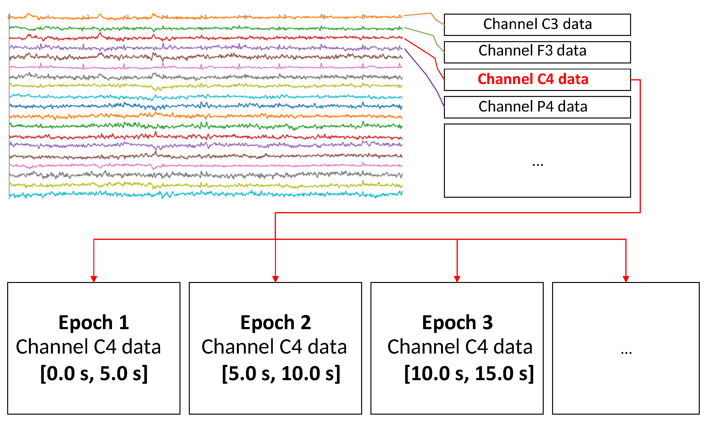
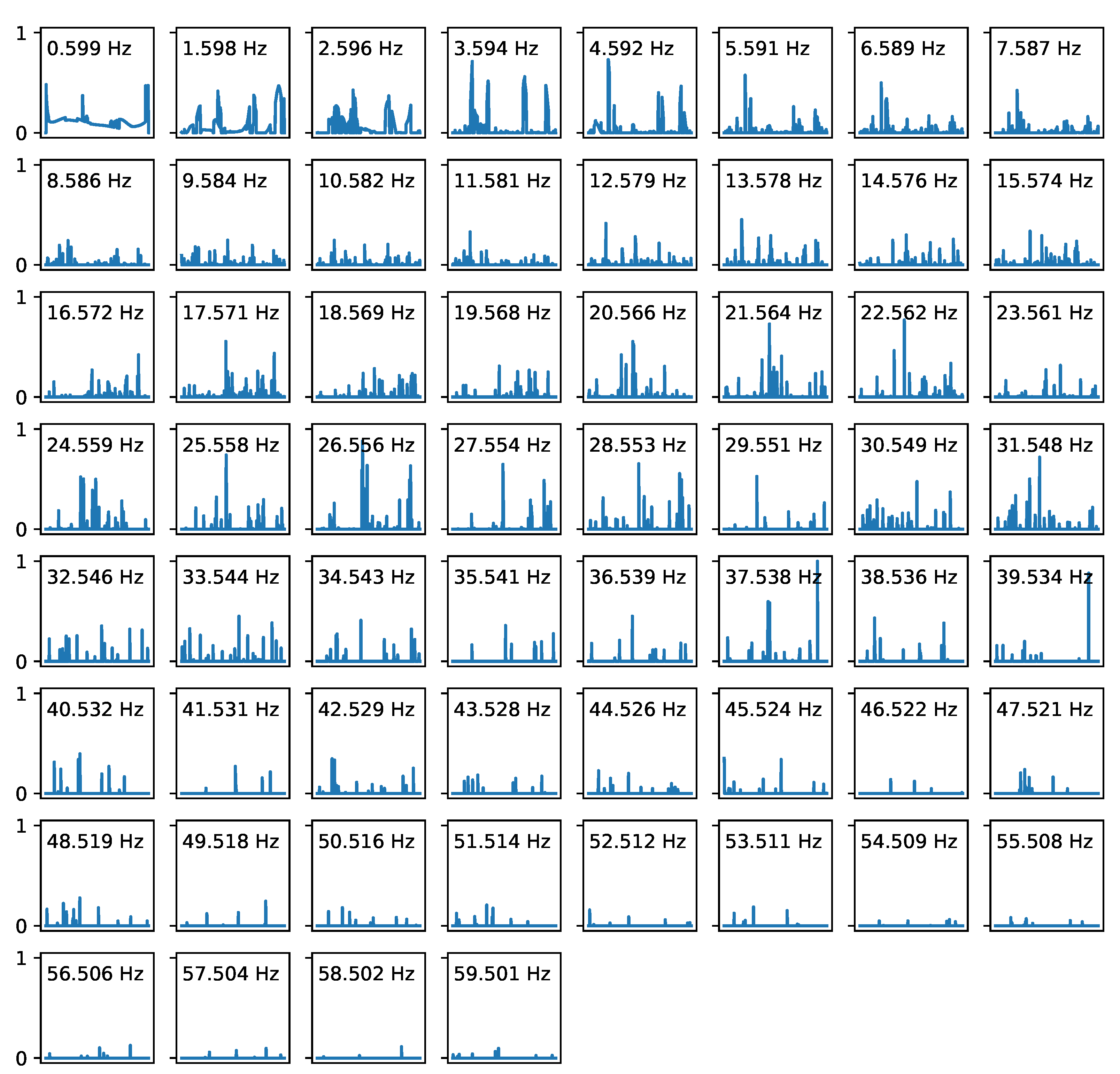
2.2. Signal Processing
2.3. Deep Learning Methods
2.4. Model Interpretation
3. Results
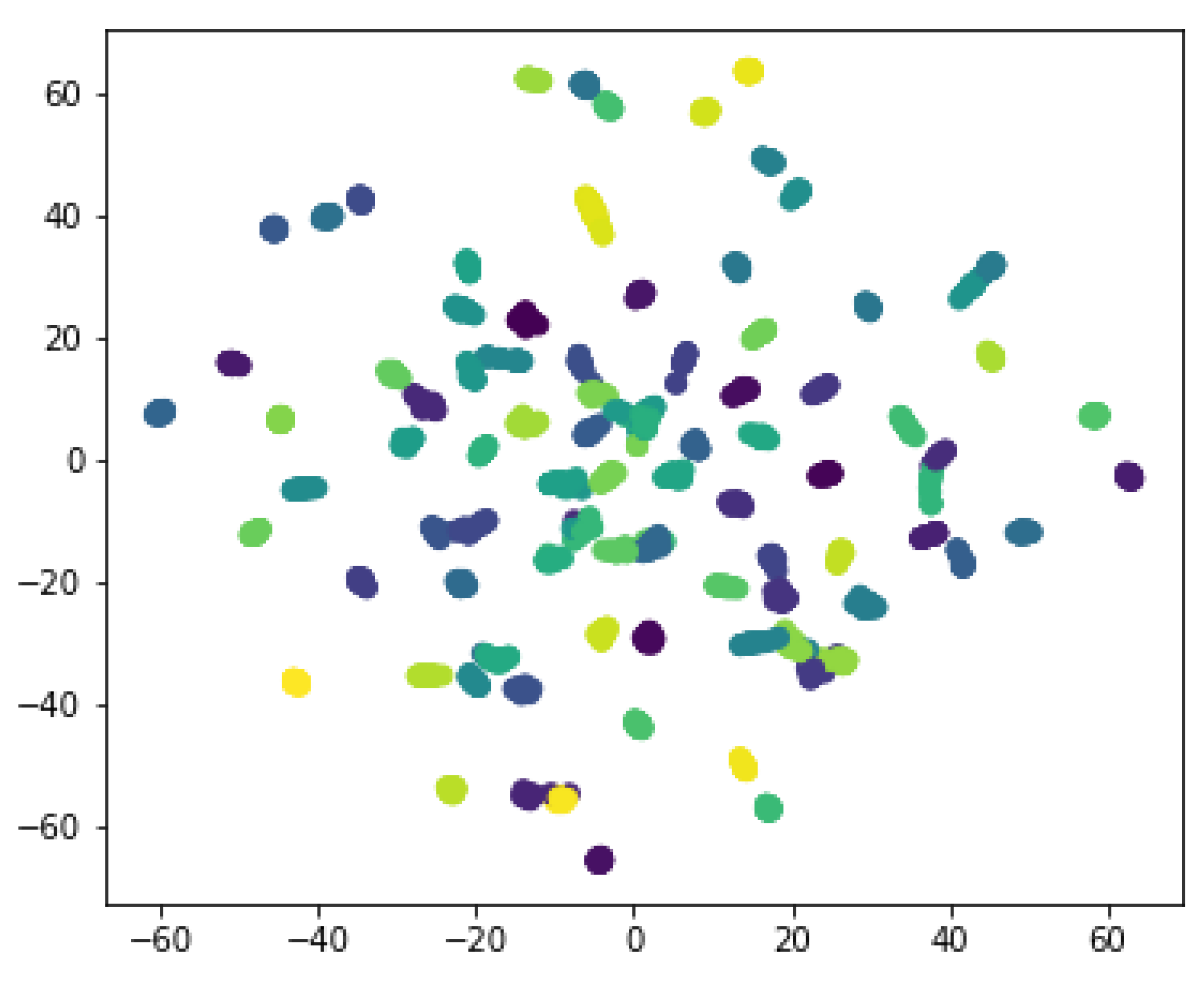
3.1. Model Training
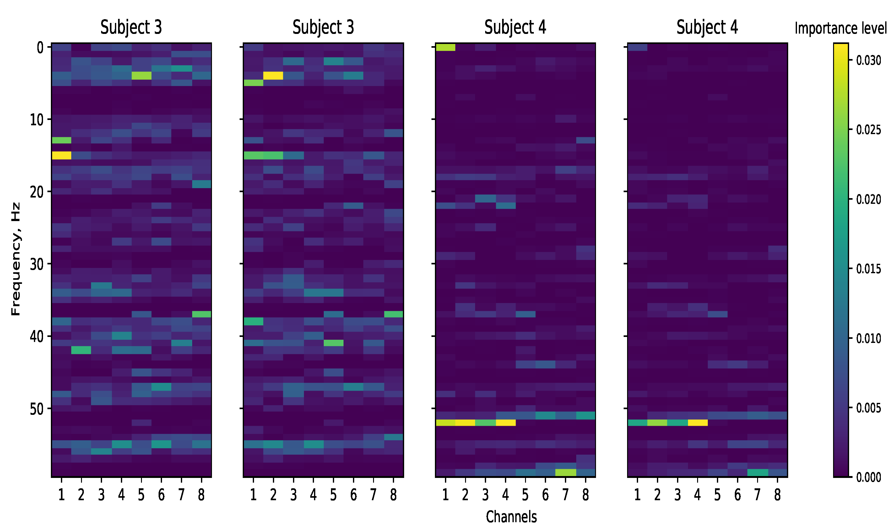
3.2. Model Interpretability
3.3. Ablation Study
4. Discussion
5. Conclusions
Author Contributions
Funding
Institutional Review Board Statement
Informed Consent Statement
Data Availability Statement
Conflicts of Interest
References
- Kodituwakku, S.R. Biometric Authentication: A Review. Int. J. Trend Res. Dev. 2015, 2, 113–123. [Google Scholar]
- Chuang, J.; Nguyen, H.; Wang, C.; Johnson, B. I Think, Therefore I Am: Usability and Security of Authentication Using Brainwaves. In Financial Cryptography and Data Security, Proceedings of the International Conference on Financial Cryptography and Data Security, Okinawa, Japan, 1–5 April 2013; Springer: Berlin/Heidelberg, Germany, 2013; Volume 7862, pp. 1–16. [Google Scholar] [CrossRef] [Green Version]
- Jain, A.K.; Ross, A.; Prabhakar, S. An Introduction to Biometric Recognition. IEEE Trans. Circuits Syst. Video Technol. 2004, 14, 4–20. [Google Scholar] [CrossRef] [Green Version]
- Hashim, M.M.; Mohsin, A.K.; Rahim, M.S.M. All-Encompassing Review of Biometric Information Protection in Fingerprints Based Steganography. In Proceedings of the 2019 3rd International Symposium on Computer Science and Intelligent Control, Amsterdam, The Netherlands, 25–27 September 2019; Association for Computing Machinery: New York, NY, USA, 2019. [Google Scholar]
- Yang, W.; Wang, S.; Sahri, N.M.; Karie, N.M.; Ahmed, M.; Valli, C. Biometrics for Internet-of-Things security: A review. Sensors 2021, 21, 6163. [Google Scholar] [CrossRef] [PubMed]
- Gui, Q.; Ruiz-Blondet, M.V.; Laszlo, S.; Jin, Z. A Survey on Brain Biometrics. ACM Comput. Surv. 2019, 51, 1–38. [Google Scholar] [CrossRef]
- Hartmann, K.G.; Schirrmeister, R.T.; Ball, T. EEG-GAN: Generative adversarial networks for electroencephalograhic (EEG) brain signals. arXiv 2018, arXiv:1806.01875. [Google Scholar]
- Satapathy, S.K.; Bhoi, A.K.; Loganathan, D.; Khandelwal, B.; Barsocchi, P. Machine learning with ensemble stacking model for automated sleep staging using dual-channel EEG signal. Biomed. Signal Process. Control 2021, 69, 102898. [Google Scholar] [CrossRef]
- Hussain, I.; Park, S.J. Quantitative Evaluation of Task-Induced Neurological Outcome after Stroke. Brain Sci. 2021, 11, 900. [Google Scholar] [CrossRef] [PubMed]
- Hussain, I.; Park, S.J. HealthSOS: Real-Time Health Monitoring System for Stroke Prognostics. IEEE Access 2020, 8, 213574–213586. [Google Scholar] [CrossRef]
- Hussain, I.; Park, S.J. Big-ECG: Cardiographic Predictive Cyber-Physical System for Stroke Management. IEEE Access 2021, 9, 123146–123164. [Google Scholar] [CrossRef]
- Paul, S.; Saikia, A.; Hussain, M.; Barua, A.R. EEG-EMG Correlation for Parkinson’s disease. Int. J. Eng. Adv. Technol. 2019, 8, 1179–1185. [Google Scholar] [CrossRef]
- Oh, S.L.; Hagiwara, Y.; Raghavendra, U.; Yuvaraj, R.; Arunkumar, N.; Murugappan, M.; Acharya, U.R. A deep learning approach for Parkinson’s disease diagnosis from EEG signals. Neural Comput. Appl. 2018, 32, 10927–10933. [Google Scholar] [CrossRef]
- Lee, Y.Y.; Hsieh, S. Classifying Different Emotional States by Means of EEG-Based Functional Connectivity Patterns. PLoS ONE 2014, 9, e95415. [Google Scholar] [CrossRef] [PubMed]
- Song, T.; Zheng, W.; Song, P.; Cui, Z. EEG Emotion Recognition Using Dynamical Graph Convolutional Neural Networks. IEEE Trans. Affect. Comput. 2020, 11, 532–541. [Google Scholar] [CrossRef] [Green Version]
- Kumaran, D.S. Using EEG-Validated Music Emotion Recognition Techniques to Classify Multi-Genre Popular Music for Therapeutic Purposes. 2018. Available online: https://digitalcommons.imsa.edu/cgi/viewcontent.cgi?article=1023&context=issf2018 (accessed on 30 November 2021).
- Fan, J.; Wade, J.W.; Key, A.P.; Warren, Z.E.; Sarkar, N. EEG-Based Affect and Workload Recognition in a Virtual Driving Environment for ASD Intervention. IEEE Trans. Biomed. Eng. 2018, 65, 43–51. [Google Scholar] [CrossRef]
- Suhaimi, N.S.; Mountstephens, J.; Teo, J. EEG-Based Emotion Recognition: A State-of-the-Art Review of Current Trends and Opportunities. Comput. Intell. Neurosci. 2020, 2020, 1–19. [Google Scholar] [CrossRef] [PubMed]
- Mason, J.; Dave, R.; Chatterjee, P.; Graham-Allen, I.; Esterline, A.; Roy, K. An investigation of biometric authentication in the healthcare environment. Array 2020, 8, 100042. [Google Scholar] [CrossRef]
- Poulos, M.; Rangoussi, M.; Alexandris, N.; Evangelou, A. On the use of EEG features towards person identification via neural networks. Med. Inf. Internet Med. 2001, 26, 35–48. [Google Scholar] [CrossRef] [Green Version]
- Zhi Chin, T.; Saidatul, A.; Ibrahim, Z. Exploring EEG based Authentication for Imaginary and Non-imaginary tasks using Power Spectral Density Method. IOP Conf. Ser. Mater. Sci. Eng. 2019, 557, 012031. [Google Scholar] [CrossRef]
- Wu, Q.; Zeng, Y.; Zhang, C.; Tong, L.; Yan, B. An EEG-Based Person Authentication System with Open-Set Capability Combining Eye Blinking Signals. Sensors 2018, 18, 335. [Google Scholar] [CrossRef] [Green Version]
- Kaliraman, B.; Duhan, M. A new hybrid approach for feature extraction and selection of electroencephalogram signals in case of person recognition. J. Reliab. Intell. Environ. 2021, 7, 241–251. [Google Scholar] [CrossRef]
- Maiorana, E.; La Rocca, D.; Campisi, P. On the permanence of EEG signals for biometric recognition. IEEE Trans. Inf. Forensics Secur. 2016, 11, 163–175. [Google Scholar] [CrossRef]
- Maiorana, E. EEG-Based Biometric Verification Using Siamese CNNs. In New Trends in Image Analysis and Processing—ICIAP 2019; Springer: Cham, Switzerland, 2019. [Google Scholar] [CrossRef]
- Maiorana, E. Learning deep features for task-independent EEG-based biometric verification. Pattern Recognit. Lett. 2021, 143, 122–129. [Google Scholar] [CrossRef]
- Barayeu, U.; Horlava, N.; Libert, A.; Van Hulle, M. Robust single-trial EEG-based authentication achieved with a 2-stage classifier. Biosensors 2020, 10, 124. [Google Scholar] [CrossRef] [PubMed]
- Sundararajan, M.; Taly, A.; Yan, Q. Axiomatic Attribution for Deep Networks. In Proceedings of the International Conference on Machine Learning, Sydney, Australia, 6–11 August 2017. [Google Scholar]
- Arrieta, A.B.; Díaz-Rodríguez, N.; Ser, J.D.; Bennetot, A.; Tabik, S.; Barbado, A.; García, S.; Gil-López, S.; Molina, D.; Benjamins, R.; et al. Explainable Artificial Intelligence (XAI): Concepts, Taxonomies, Opportunities and Challenges toward Responsible AI. Inf. Fusion 2020, 58, 82–115. [Google Scholar] [CrossRef] [Green Version]
- Schalk, G.; McFarland, D.J.; Hinterberger, T.; Birbaumer, N.; Wolpaw, J.R. BCI2000: A general-purpose brain-computer interface (BCI) system. IEEE Trans. Biomed. Eng. 2004, 51, 1034–1043. [Google Scholar] [CrossRef]
- Larson, E.; Gramfort, A.; Engemann, D.A.; Jaeilepp; Brodbeck, C.; Jas, M.; Brooks, T.L.; Sassenhagen, J.; Luessi, M.; King, J.R.; et al. MNE-Tools/MNE-Python: v0.24.1. 2021. Available online: https://mne.tools/stable/index.html (accessed on 30 November 2021).
- Zhang, L.; Wu, D.; Zhi, L. Method of removing noise from EEG signals based on HHT method. In Proceedings of the 2009 First International Conference on Information Science and Engineering, Nanjing, China, 26–28 December 2009. [Google Scholar]
- Souza, U.B.D.; Escola, J.P.L.; Brito, L.D.C. A survey on Hilbert–Huang transform: Evolution, challenges and solutions. Digit. Signal Process. 2022, 120, 103292. [Google Scholar] [CrossRef]
- Deering, R.; Kaiser, J.F. The use of a masking signal to improve empirical mode decomposition. In Proceedings of the (ICASSP’05)—IEEE International Conference on Acoustics, Speech, and Signal Processing, Philadelphia, PA, USA, 23 March 2005. [Google Scholar]
- Quinn, A.J.; Lopes-dos Santos, V.; Dupret, D.; Nobre, A.C.; Woolrich, M.W. EMD: Empirical Mode Decomposition and Hilbert–Huang Spectral Analyses in Python. J. Open Source Softw. 2021, 6, 2977. [Google Scholar] [CrossRef] [PubMed]
- Ruffini, G.; Ibañez, D.; Castellano, M.; Dubreuil-Vall, L.; Soria-Frisch, A.; Postuma, R.; Gagnon, J.F.; Montplaisir, J. Deep Learning With EEG Spectrograms in Rapid Eye Movement Behavior Disorder. Front. Neurol. 2019, 10, 806. [Google Scholar] [CrossRef] [Green Version]
- Yazdanbakhsh, O.; Dick, S. Multivariate Time Series Classification using Dilated Convolutional Neural Network. arXiv 2019, arXiv:1905.01697. [Google Scholar]
- Musgrave, K.; Belongie, S.; Lim, S.N. A Metric Learning Reality Check. In European Conference on Computer Vision; Springer: Cham, Switzerland, 2020. [Google Scholar]
- Hoffer, E.; Ailon, N. Deep metric learning using Triplet network. In International Workshop on Similarity-Based Pattern Recognition; Springer: Cham, Switzerland, 2015. [Google Scholar]
- Deng, J.; Guo, J.; Xue, N.; Zafeiriou, S. ArcFace: Additive Angular Margin Loss for Deep Face Recognition. In Proceedings of the IEEE/CVF Conference on Computer Vision and Pattern Recognition, Long Beach, CA, USA, 15–20 June 2019. [Google Scholar]
- Wang, X.; Han, X.; Huang, W.; Dong, D.; Scott, M.R. Multi-Similarity Loss with General Pair Weighting for Deep Metric Learning. In Proceedings of the IEEE/CVF Conference on Computer Vision and Pattern Recognition, Long Beach, CA, USA, 15–20 June 2019. [Google Scholar]
- He, K.; Zhang, X.; Ren, S.; Sun, J. Delving Deep into Rectifiers: Surpassing Human-Level Performance on ImageNet Classification. In Proceedings of the IEEE International Conference on Computer Vision, Santiago, Chile, 7–13 December 2015. [Google Scholar]
- Kokhlikyan, N.; Miglani, V.; Martin, M.; Wang, E.; Alsallakh, B.; Reynolds, J.; Melnikov, A.; Kliushkina, N.; Araya, C.; Yan, S.; et al. Captum: A unified and generic model interpretability library for PyTorch. arXiv 2020, arXiv:2009.07896. [Google Scholar]
- Pedregosa, F.; Varoquaux, G.; Gramfort, A.; Michel, V.; Thirion, B.; Grisel, O.; Blondel, M.; Prettenhofer, P.; Weiss, R.; Dubourg, V.; et al. Scikit-learn: Machine Learning in Python. J. Mach. Learn. Res. 2011, 12, 2825–2830. [Google Scholar]
- Maiorana, E.; Campisi, P. Longitudinal evaluation of EEG-based biometric recognition. IEEE Trans. Inf. Forensics Secur. 2018, 13, 1123–1138. [Google Scholar] [CrossRef]
- van der Maaten, L.; Hinton, G.E. Visualizing Data using t-SNE. J. Mach. Learn. Res. 2008, 9, 2579–2605. [Google Scholar]
- Chollet, F. Keras. 2015. Available online: https://github.com/fchollet/keras (accessed on 30 November 2021).
- Harris, C.R.; Millman, K.J.; van der Walt, S.J.; Gommers, R.; Virtanen, P.; Cournapeau, D.; Wieser, E.; Taylor, J.; Berg, S.; Smith, N.J.; et al. Array programming with NumPy. Nature 2020, 585, 357–362. [Google Scholar] [CrossRef] [PubMed]
- Hunter, J.D. Matplotlib: A 2D graphics environment. Comput. Sci. Eng. 2007, 9, 90–95. [Google Scholar] [CrossRef]
- Schalk, G.; McFarland, D.J.; Hinterberger, T.; Birbaumer, N.; Wolpaw, J.R. EEG Motor Movement/Imagery Dataset. 2009. Available online: https://physionet.org/content/eegmmidb/1.0.0/ (accessed on 30 November 2021).


| Layer | Output Shape | Trainable Parameters |
|---|---|---|
| Dropout(dr = 0.7) | (480, 801) | 0 |
| Conv1d(f = 512,k = 5,d = 1,p = “same”) | (512, 801) | 1,229,312 |
| BatchNorm1d | (512, 801) | 1024 |
| PReLU | (512, 801) | 512 |
| Conv1d(f = 512,k = 5,d = 2) | (512, 801) | 655,616 |
| BatchNorm1d | (512, 801) | 512 |
| PReLU | (256, 801) | 256 |
| Conv1d(f = 512,k = 5,d = 4) | (256, 777) | 327,936 |
| BatchNorm1d | (256, 777) | 512 |
| PReLU | (256, 777) | 256 |
| Conv1d(f = 512,k = 5,d = 16) | (256, 777) | 327,936 |
| BatchNorm1d | (256, 713) | 512 |
| PReLU | (256, 713) | 256 |
| Dropout(dr = 0.7) | (256, 713) | 0 |
| Conv1d(f = 512,k = 5,d = 32) | (256, 585) | 327,936 |
| BatchNorm1d | (256, 585) | 512 |
| PReLU | (256, 585) | 256 |
| Conv1d(f = 512,k = 5,d = 72) | (256, 297) | 327,936 |
| BatchNorm1d | (256, 297) | 512 |
| PReLU | (256, 297) | 256 |
| Conv1d(f = 512,k = 5,d = 74) | (256, 1) | 327,936 |
| BatchNorm1d | (256, 1) | 512 |
| PReLU | (256, 1) | 256 |
| FullyConnected(n = 256) | (256, 1) | 65,792 |
| PReLU | (256) | 256 |
| FullyConnected(n = 128) | (128, 1) | 32,896 |
| Frequency Range | 0–10 Hz | 10–20 Hz | 20–30 Hz | 30–40 Hz | 40–50 Hz | 50–60 Hz |
|---|---|---|---|---|---|---|
| Accuracy | 74.2% | 73.5% | 72.8% | 74.9% | 72.9% | 68.2% |
Publisher’s Note: MDPI stays neutral with regard to jurisdictional claims in published maps and institutional affiliations. |
© 2022 by the authors. Licensee MDPI, Basel, Switzerland. This article is an open access article distributed under the terms and conditions of the Creative Commons Attribution (CC BY) license (https://creativecommons.org/licenses/by/4.0/).
Share and Cite
Svetlakov, M.; Kovalev, I.; Konev, A.; Kostyuchenko, E.; Mitsel, A. Representation Learning for EEG-Based Biometrics Using Hilbert–Huang Transform. Computers 2022, 11, 47. https://doi.org/10.3390/computers11030047
Svetlakov M, Kovalev I, Konev A, Kostyuchenko E, Mitsel A. Representation Learning for EEG-Based Biometrics Using Hilbert–Huang Transform. Computers. 2022; 11(3):47. https://doi.org/10.3390/computers11030047
Chicago/Turabian StyleSvetlakov, Mikhail, Ilya Kovalev, Anton Konev, Evgeny Kostyuchenko, and Artur Mitsel. 2022. "Representation Learning for EEG-Based Biometrics Using Hilbert–Huang Transform" Computers 11, no. 3: 47. https://doi.org/10.3390/computers11030047
APA StyleSvetlakov, M., Kovalev, I., Konev, A., Kostyuchenko, E., & Mitsel, A. (2022). Representation Learning for EEG-Based Biometrics Using Hilbert–Huang Transform. Computers, 11(3), 47. https://doi.org/10.3390/computers11030047