Multi-Period Optimal Reactive Power Dispatch Using a Mean-Variance Mapping Optimization Algorithm

Abstract

Optimal reactive power dispatch plays a key role in the safe operation of electric power systems. It consists of the optimal management of the reactive power sources within the system, usually with the aim of reducing system power losses. This paper presents both a new model and a solution approach for the multi-period version of the optimal reactive power dispatch. The main feature of a multi-period approach lies on the incorporation of inter-temporal constraints that allow the number of switching operations in transformer taps and capacitor banks to be limited in order to preserve their lifetime and avoid maintenance cost overruns. The main contribution of the paper is the constraint handling approach which consists of a multiplication of sub-functions which act as penalization and allow simultaneous consideration of both the feasibility and optimality of a given candidate solution. The multi-period optimal reactive power dispatch is an inherently nonconvex and nonlinear problem; therefore, it was solved using the metaheuristic mean-variance mapping optimization algorithm. The IEEE 30-bus and IEEE 57-bus test systems were used to validate the model and solution approach. The results allow concluding that the proposed model guarantees an adequate reactive power management that meets the objective of minimizing power losses and keeping the transformer taps and capacitor bank movements within limits that allow guaranteeing their useful life.

1. Introduction

The optimal reactive power dispatch (ORPD) consists of the management of reactive generation and voltage control resources of a power system usually with the aim of minimizing power loses. The ORPD is carried out after the scheduling of the active power dispatch and must be performed without altering it; with the exception of the reference bus that must compensate power losses [1]. Although the main objective of the ORPD is power loss reduction, other objectives—such as improving voltage profile, minimizing voltage deviation from a given value, and improving voltage stability—may be considered [2].

From the standpoint of mathematical optimization, the ORPD is a mixed integer nonlinear programming problem which combines discrete control variables such as tap setting transformers and reactive compensators, and continuous variables such as generator bus voltage set points [3]. The first attempts to solve the ORPD resorted to classical optimization techniques, such as linear programming [4], nonlinear programming [5], quadratic programming [6,7], interior point method [8], Newton-based method [9,10], gradient-based algorithm [11], and decomposition approach [12]. Despite their optimal results in other fields, when solving the ORPD, these techniques are easily trapped in local optimal solutions due to the nonlinear and nonconvex nature of the ORPD problem. Furthermore, classic optimization techniques are unable to tackle problems with discontinuous and non-differentiable objective functions, as well as discrete decision variables. These type of problems are better handled by metaheuristic optimization techniques, as evidenced in [2,13,14]. Metaheuristic algorithms are usually inspired by natural or physical phenomena, such as animal behavior, evolution, gravitational force, electromagnetic force, etc. These techniques have become popular due to their ability to tackle highly complex optimization problems, overcoming the shortcomings of classical optimization techniques. Several of these metaheuristic techniques have been applied to the ORPD problem.

Bat optimization is inspired by the behavior of bats that use echolocation to find food. This technique uses a frequency-tuning technique to control the dynamic behavior of a swarm of bats. In [2], the authors proposed a chaotic bat algorithm to solve the ORPD in medium and large-scale power systems. In this case, chaotic sequences are introduced into the standard bat algorithm to enhance its global search ability.

Evolutionary and genetic algorithms (GA) are inspired on Darwinian evolution and feature robustness and flexibility for solving complex optimization problems [15]. A GA begins with a randomly selected set of candidate solutions that must go to the phases of selection reconfiguration and mutation to find new and better solutions until a stopping criterion is met. In [16], the authors propose a composite differential evolution technique to solve the ORPD considering several wind and demand scenarios. In [17], a real coded GA is proposed to solve the ORPD problem. In [18], a multi-objective GA is proposed to solve the ORPD; in [18], the authors present a real-time optimization of reactive power using a GA. Other applications of GAs to solve the ORPD problem are reported in [17,19,20].

Gray wolf optimization mimics the leadership hierarchy and hunting mechanisms of gray wolves in nature. This technique is applied in [21] to solve the ORPD. In this case, transmission losses, voltage deviation, and a stability index are considered.

Swarm intelligence refers to complex systems of multiple agents or populations (birds, ants, bees, etc.) that contain numerous numerous individuals, which exhibit intelligent behavior through cooperation and competition among them. The most representative algorithms within this category are particle swarm optimization (PSO), ant colony optimization (ACO), and artificial bee colony (ABC) optimization. In [22,23], the authors implement PSO to solve the ORP dispatch. A firefly algorithm is proposed in [24] to solve the multi-objective optimal active/reactive power dispatch considering uncertainties. In [25], ABC is applied to solve the short-term reactive power procurement considering voltage stability issues. In [26], the ABC optimization is applied to solve the combined active/reactive power dispatch problem.

There are optimization algorithms that are inspired by physical laws (forces between electrical charges, gravity, river systems, etc.). Although there are many metaheuristic optimization methods that are based on physical phenomena, they have not been widely applied to the ORPD. A gravitational search algorithm (GSA) is proposed in [27] to solve the optimal reactive power dispatch; while in [28] the authors propose an opposition-based, self-adaptive, modified GSA to solve the multiobjective optimal reactive power dispatch. In [29], a harmony search algorithm is proposed to solve the ORPD problem, while in [30] a charged system algorithm is developed for the same purpose.

Hybrid metaheuristic algorithms combine the strengths of two or more techniques to facilitate the solution of complex optimization problems. In [31], the authors propose a hybrid GA-interior point method to solve the optimal reactive power flow. The ORPD is divided in two steps. The first step solves the ORPF with the interior point method relaxing discrete variables. The step decomposes the original ORPF into a continuous and a discrete optimization problem. In [32], the authors combined differential evolution algorithm with ACO to solve the optimal reactive power dispatch. In [33], PSO is hybridized with a GA with real coding to solve the ORPD problem. In [34], the authors present a fractional PSO combined with a GSA to minimize power line losses and voltage deviation. Other hybrid PSO approaches are explored in [35,36,37]. A detail description of all techniques applied to solve the ORPD is out of the scope of this paper; nonetheless, a review of metaheuristics applied to the ORPD can be consulted in [38].

The multi-period version of the ORPD (MP-ORPD) encompasses several time intervals and is usually planed for 24 h. The MP-ORPD is a more challenging problem than its single-period counterpart since it implies constraints regarding the total number of maneuvers in transformer taps, capacitor, and reactor banks throughout the time interval considered. The MP-OPRP is carried out after the execution of a unit commitment (UC) process [39,40]. The UC can be described as a multi-period optimal power dispatch where active power is adjudicated to generators as function of their price offers (bids) and limits. The UC, executed prior to the MP-ORPD, may take into account the presence of renewable generation [41,42]. In this case, the expected active power injections are inputs to the MP-ORPD, which is envisaged not to alter the previous active dispatch found by the UC—with the exception the slack bus that must account for power losses.

Being a more challenging optimization problem, there are few studies that approach the MP-ORPD. Some of the methodologies used to solve this problem include interior point methods [43,44,45], genetic algorithms [46], artificial electric field algorithm [47], dynamic programming [48,49], mathematical programming approaches [50,51,52,53], and decomposition techniques [54]. The main modeling aspects considered in the aforementioned studies are summarized in

Table 1. Main modeling aspects considered in MP-ORPD approaches.

Paper	Transformers		Reactive Compensation		Stopping Criterion
	Daily	Inter-Hour	Daily	Inter-Hour	Number of Evaluations	Goal Accomplished
[43]	X	X		X	X
[44,46,48,50]		X		X	X
[45,49,51,52,53,54]	X		X		X
[47]			X		X
Proposed	X	X	X	X	X	X

. Note that the proposed approach complements other works presented in the specialized literature based on the fact that that the stopping criterion is not only a given number of evaluations but also a goal accomplished. Furthermore, daily and inter-hour constraints are considered for both transformer and reactive compensation banks.

As main contributions, this paper proposes a new model and solution approach for the MP-ORPD. One of the special features of the proposed approach is the constraint handling approach that complements the one proposed in [55] initially proposed for the single-period ORPD. In this case, the objective function along with the constraints consist on a multiplications of sub-functions. A goal on power loss reduction is set at the beginning of the algorithm. If a given candidate solution complies with the goal of power losses and with all constraints, then the result of the multiplication is one (meaning that the problem is both feasible and optimal); otherwise the multiplication is less than one. This feature facilitates the optimization process and allows us to easily verify the quality of a given candidate solution. Furthermore, the number of switching operations in transformer taps and capacitor banks is limited according to data recommended by the manufacturer in order to preserve the lifetime of these devices and avoid maintenance costs overruns. A mean-variance mapping optimization (MVMO) is used to solve the proposed MP-ORPD model. It is worth mentioning that the effectiveness and applicability of the MVMO algorithm to solve the single-period ORPD was proven by the authors in [56] where it was compared with other metaheuristic approaches that include artificial bee colony (ABC), firefly algorithm (FA), differential evolution (DE), comprehensive learning particle swarm optimization (CLPSO), biogeography-based optimization (BBO), and improved gravitational search algorithm (IGSA). The rest of the document is organized as follows: Section 2 presents the mathematical modeling of the MP-ORPD; Section 3 describes the solution approach based on a MVMO technique; Section 4 presents the tests and results in two benchmark power systems; finally, Section 5 presents the conclusions of the work.

2. Mathematical Modeling

The mathematical formulation of the MP-ORPD presented in this paper is an extension of the formulation presented in [55]. In this case, new constraints are added to account for maximum number of daily maneuvers in transformers and shunt elements; furthermore, the objective function is also modified to consider the enforcement of inter-temporal constraints.

2.1. Objective Function

The objective function given by Equation (1) is a multiplication of several sub-functions over a time horizon of 24 h. One of the terms is a daily loss reduction target indicated as $f_{Lossd}$. The other terms allow an alternative handling of constraints related to voltage limits at system nodes, as well as apparent power flows and number of maneuvers on transformers taps. In this case, $f_{VN}(i,t)$ and $f_{CL}(j,t)$ are sub-functions that indicate limits on voltage magnitudes at node i, and apparent power flows in line j for time period t, respectively. $f_{CTh}(i,t)$ is the sub-function that indicates limits on number of maneuvers in transformer k at time period t.

$$OF={\displaystyle \prod _{t=1}^{24}}\left\{{\displaystyle \prod _{i=1}^{N_L}}{f}_{VN}(i,t){\displaystyle \prod _{j=1}^{N_K}}{f}_{CL}(j,t){\displaystyle \prod _{k=1}^{N_T}}{f}_{CTh}(k,t)\right\}{f}_{lossd}\left\{{\displaystyle \prod _{k=1}^{N_T}}{f}_{CTd}\left(k\right){\displaystyle \prod _{l=1}^{N_C}}{f}_{CCd\left(l\right)}\right\}$$

(1)

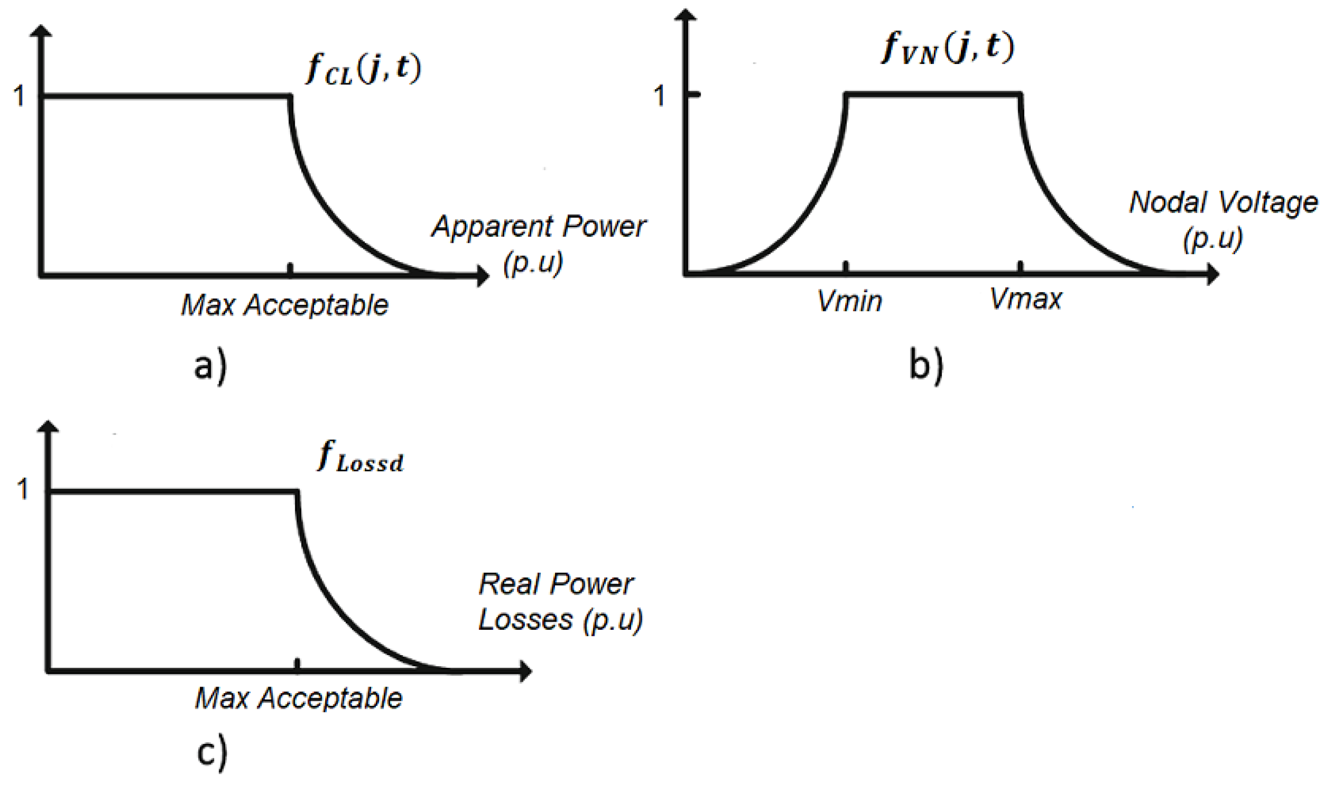
2.2. Enforcement of Voltage Limits

The mathematical expression of the sub-function that controls voltage limits is given by Equation (2). In this case $V_{mini}$ and $V_{maxi}$ are the minimum and maximum voltage limits at bus i, respectively; $\lambda v$ is is a penalty constant for voltage deviations, and $V_{i,t}$ is the voltage of bus i at time interval t.

$$f_{VN}(i,t)=\left\{\begin{array}{c}{e}^{\lambda v(V_{maxi}-V_{i,t}),V_{i,t}>V_{maxi}}\hfill \\ e^{\lambda v(V_{i,t}-V_{mini}),V_{mini}>V_{i,t}}\hfill \\ 1,V_{mini}\le V_{i,t}\le V_{maxi}\hfill \end{array}\right\}$$

(2)

2.3. Enforcement of Power Flow Limits

The sub-function that enforces apparent power flow limits is given by Equation (3). In this case, $\lambda b$ is a penalty factor for power flows out of limits, $Loa{d}_{Rjmax}$ is the maximum apparent power flow allowed by transmission line j, and $Loa{d}_{Rj,t}$ is the apparent power flow of line j at time interval t.

$$f_{CL}(j,t)=\left\{\begin{array}{c}{e}^{\lambda b(Loa{d}_{Rjmax}-Loa{d}_{Rj,t}),Loa{d}_{Rj,t}>Loa{d}_{Rjmax}}\hfill \\ 1,Loa{d}_{Rj,t}\le Loa{d}_{Rjmax}\hfill \end{array}\right\}$$

(3)

2.4. Active Power Losses Target

The goal of active power losses, defined by the system operator, is given by Equation (4). In this case, $\lambda l$ is a penalty factor for power losses greater than the target defined by the system operator, $Los{s}_R$ represents the daily total power losses of the system, and $P_{lossd}$ is the target of daily power losses.

$$f_{lossd}=\left\{\begin{array}{c}{e}^{\lambda l(Los{s}_R-P_{lossd}),P_{lossd}>Los{s}_R}\hfill \\ 1,P_{lossd}\le {Loss}_R\hfill \end{array}\right\}$$

(4)

Figure 1 illustrates the sub-functions used to evaluate limits on voltages, apparent power flows, and the goal on daily power losses. It is important to note that the sub-functions described below for transformer taps switching constraints and for daily capacitor switching limits feature a similar shape as those illustrated in Figure 1.

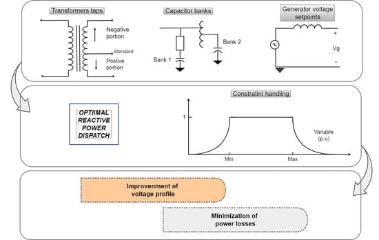
2.5. Limits on Transformer Taps Maneuvers

Equations (5)–(8) enforce the limits on number of transformer maneuvers. In this case, ${\lambda }_{CT}$, $C_{Maxh,T,k}$ and $C_{OT}(k,t)$ are the exponential penalty factor for deviations from the maximum allowed transformer maneuvers, the maximum cost of hourly maneuvers allowed in the k-th transformer and the hourly operating cost for maneuvers performed in the k-th transformer in period t, respectively. The last two expressions are given by Equations (6) and (7), respectively; where $C{T}_k$ is the cost of operating the k-th transformer, $T_{maxh,k}$ is the maximum number of operations allowed for the k-th transformer, $N{T}_{k,t}$ is the number of operations performed by the k-th transformer in the period t, and $P_{base}$ is the active base power. Equation (8) indicates the number tap positions moved within two consecutive time periods of a given transformer.

$$f_{CT}(k,t)=\left\{\begin{array}{c}{e}^{\left[{\lambda }_{CT}\left(C_{Maxh,T,k}-C_{OT}(k,t)\right)\right],C_{OT}(k,t)>Maxh,T,k}\hfill \\ 1,C_{OT}(k,t)\le C_{Maxh,T,k}\hfill \end{array}\right\}$$

(5)

$$C_{Maxh,T,k}=\frac{C{T}_k{T}_{maxh,k}}{P_{base}}$$

(6)

$$C_{OT}(k,t)=\frac{C{T}_{k}N{T}_{k,t}}{P_{base}}$$

(7)

$$N{T}_{k,t}=\left|Ta{p}_{k,t}-Ta{p}_{k,t-1}\right|,k=1,...,T,t=1,...,24 \mathrm{h}$$

(8)

2.6. Daily Limit of Transformer Tap Operations

A maximum number of daily operations is defined for each transformer in order to preserve their lifetime and avoid maintenance cost overruns. Equations (9) and (10) enforce the maximum daily switching operations of transformers. In this case, ${\lambda }_{CT}$ is an exponential penalty factor for number of tap operations out of limits, $C_{Maxd,T,k}$ is the maximum daily switching cost allowed for the k-th transformer, and $C_{OT}(k,t)$ is the switching cost of transformer k in time interval t. In Equation (10), $C{T}_k$ is the cost of operating the k-th transformer, and $T{max}_{d,k}$ is the maximum number of daily operations allowed for the k-th transformer.

$$f_{CTd}\left(k\right)=\left\{\begin{array}{c}{e}^{\left[{\lambda }_{CT}\left(C_{Maxd,T,k}-{\sum }_{t=1}^{24}{C}_{OT}(k,t)\right)\right],{\sum }_{t=1}^{24}{C}_{OT}(k,t)>C_{Maxd,T,k}}\hfill \\ 1,{\sum }_{t=1}^{24}{C}_{OT}(k,t)\le C_{Maxd,T,k}\hfill \end{array}\right\}$$

(9)

$$C_{Maxd,T,k}=\frac{C{T}_{k}T{max}_{d,k}}{P_{base}}$$

(10)

2.7. Capacitor Banks Daily Switching Limit

The number of maneuvers in capacitor banks must also be limited to avoid affecting its useful life and reduce maintenance costs. The enforcement of switching limits on capacitor banks are given by Equations (11)–(14). In this case, ${\lambda }_{CC}$ is an exponential penalty factor for number of capacitor maneuvers out of limits, $C_{Maxd,C,l}$ is the maximum number of daily maneuvers in a capacitor bank, $C_{OC}(l,t)$ is the cost of hourly maneuvers performed by the l-th capacitor bank. In Equation (12), $C{C}_l$ is is the cost of operating the l-th capacitor bank and $C{max}_{d,l}$ is the maximum daily number of switching operations allowed for the l-th capacitor bank. In Equation (13), $N{C}_{l,t}$ is the number of hourly switching operations performed by the l-th capacitor bank in the period t, and in Equation (14), $C_{l,t}$, $C_{l,t-1}$, and $\Delta C$ are reactive power capacity injected by the l-th capacitor bank in time t and time $t-1$, and the reactive power injection step of the l-th capacitor bank, respectively.

$$f_{CCd}\left(k\right)=\left\{\begin{array}{c}{e}^{\left[{\lambda }_{CC}\left(C_{Maxd,C,l}-{\sum }_{t=1}^{24}{C}_{OC}(l,t)\right)\right],{\sum }_{t=1}^{24}{C}_{OC}(l,t)>C_{Maxd,C,l}}\hfill \\ 1,{\sum }_{t=1}^{24}{C}_{OC}(l,t)\le C_{Maxd,C,l}\hfill \end{array}\right\}$$

(11)

$$C_{Maxd,C,l}=\frac{C{C}_{l}C{max}_{d,l}}{P_{base}}$$

(12)

$$C_{OC}(l,t)=\frac{C{C}_{l}N{C}_{l,t}}{Pbase}$$

(13)

$$N{C}_{l,t}=\frac{\left|C_{l,t}-C_{l,t-1}\right|}{\Delta C},l=1,...,Ct=1,...,24$$

(14)

3. Solution Approach

The MP-ORPD is a nonlinear and nonconvex optimization problem. These type of problems are better handled by metaheuristic techniques than by classical mathematical optimization. In this case, the MVMO was selected since it has proven to be effective for solving the single-period ORPD problem as reported in [57,58]. Furthermore, the MVMO algorithm features faster convergence speed than others metaheuristic techniques [57].

The MVMO approach shares several similarities with other metaheuristic algorithms; however, its main feature is a special mapping function applied to transform the variable domain for mutating the offspring, which is based on the mean and variance of the n-best population. The swarm version of this algorithm includes a population of candidate solutions [58,59].

The basic MVMO operates over a set of candidate solutions, its objective is to execute a correct and accurate optimization with a minimum quantity of objective function evaluations. The inner search space of all variables within MVMO is restricted to [0, 1]. Thus, the minimum and maximum limits of the variables must be normalized in this range. During each iteration, it is not possible that any vector solution component violates the corresponding limits. To achieve this objective, a special mapping function (h-function) was developed. The inputs of this function are the means and variance of the best solutions that the MVMO has found so far. Note that the output of this mapping function will always be within the range [0, 1], avoiding violation of variable limits during the search process. The shape and mapping curves are adjusted according to the progress in the search process and the MVMO updates the candidate solution around the best solution in each step of the iteration [60]. MVMO is able to search around the best local solution with a small possibility of being trapped in a local optimal solution. The basic considerations of the MVMO metaheuristic are detailed below.

3.1. Fitness Evaluation and Constraint Handling

The chi-squared test is applied for each candidate solution. The feasibility of the solution is checked and a fitness valued is assigned. The static penalization approach is used to handle constraints. Since the control variables are self-limited, all depending variables are restricted by applying the fitness function, as indicated in Equation (15), where f is the original objective function, n is the number of constrains, $\beta$ is the order of the penalization term, $v_i$ is the penalization coefficient of the ith constraint, and $g_i$ represents the inequality constraints.

$$min{f}^{{}^{\prime }}=f+{\sum }_{i=1}^n{v}_{i}max{\left[0,g_i\right]}^{\beta }$$

(15)

3.2. Enhanced Mapping

The mapping function transforms a variable $x_i^{*}$ varied randomly with unity distribution to another variable $x_i$, which is concentrated around the mean value. The new value of the ith variable is determined by Equation (16). Where $h_x$, $h_1$, and $h_0$ are the outputs of the mapping function based on the different inputs given by Equation (17). The mapping function (h-function) is parameterized as indicated in Equation (18), where $s_1$ and $s_2$ are shape factors that allow asymmetric variations of the mapping function. Finally, the shape factor is calculated as indicated in Equation (19). In this case, $f_s$ is a scale factor that allows controlling the search process during each iteration, while ${\overline{x}}_i$ and $v_i$ are the mean and variance of the solution archive, respectively. A more detailed description on how to adjust shape and scale is presented in [61].

$$x_i=h_x+(1-h_1+h_0)x_i^{*}-h_0$$

(16)

$$h_x=h(x=x_i^{*}),h_0=h(x=0),h_1=h(x=1)$$

(17)

$$h({\overline{x}}_i,s_1,s_2,x)={\overline{x}}_i(1-e^{-x{s}_1})+(1-{\overline{x}}_i)e^{-(1-x)s_2}$$

(18)

$$s_i=-ln\left(v_i\right)f_s$$

(19)

3.3. Solution Archive

This archive constitutes the base knowledge of the algorithm to guide the search direction. Therefore, the n best individuals that the MVMO has found so far are saved in this archive. The fitness value for each individual is also saved. The following rules are adjusted to compare the generated individuals in each iteration and the existing archived solutions aiming to avoid losing high-quality solutions: (i) any feasible solution is preferred over any unfeasible solution; (ii) between two feasible solutions, the one with the best fitness value is preferred; (iii) between two unfeasible solutions, the one with the lowest fitness value is preferred. The update is only done if the new individual is better than those that are currently in the archive. Feasible solutions are located in the upper part of the archive. These solutions are organized according to their fitness value. Unfeasible solutions are organized according to their fitness and located in the lower part of the archive. Once the archive is complete with n feasible solutions, any unfeasible solution candidate would not have the chance to be saved in the archive.

3.4. Offspring Generation and Stopping Criterion

The first positioned solution in the archive (the best so far), named as xbest, is assigned as the parent. For offspring generation a variable selection is performed. MVMO searches the mean value saved in the solution archive for the best solution only in m selected directions. This means that only these dimensions of the offspring will be updated while the $D-m$ remaining dimensions take the corresponding values of xbest, being D the dimension of the problem (number of control variables). Then, mutation is carried out for each m-selected dimension. Finally, the search process of the MVMO stops after a predetermined number of fitness evaluations is carried out.

3.5. MVMO Swarm Variant

In its swarm variant, MVMO is initiated with $n_p$ particles. In this case, each particle or candidate solution has its own solution archive and mapping function. In the process, each candidate solution executes m steps to identify an optimal set of independent solutions. Later, the particles exchange information. In some cases, some particles are very close to each other, which means that there is information redundancy. This redundancy is eliminated by discarding redundant particles. As with particle swarm optimization, a local and global best ($gbest$) solution are defined. Furthermore, the normalized distance between each particle to the local best and global best solutions are calculated. The i-th particle is discarded from the process if its normalized distance is less than a certain predefined threshold. If such threshold is zero, all particles are taken into account in the whole process; otherwise, if the threshold is one all particles are discarded except from the global best. In this case, after ($m\ast n_p+n_p$) fitness evaluations only one particle, the $gbest$, remains. Intermediate threshold values entail better adaptation to any optimization problem [58].

After independent evaluation, and if the particle is further considered, its searching will be directed toward the global solution by assigning global best instead of local best solution, as parent for the particle’s offspring. The remaining steps are identical with those of the classical MVMO. Figure 2 illustrates the flowchart of the implemented methodology. A detailed description of swarm MVMO variant is presented in [58,62].

4. Tests and Results

To show the effectiveness and applicability of the proposed approach several tests were carried out with two benchmark power systems: namely, the IEEE 30 and 57 bus test systems. This section details the application of the proposed model and solution approach.

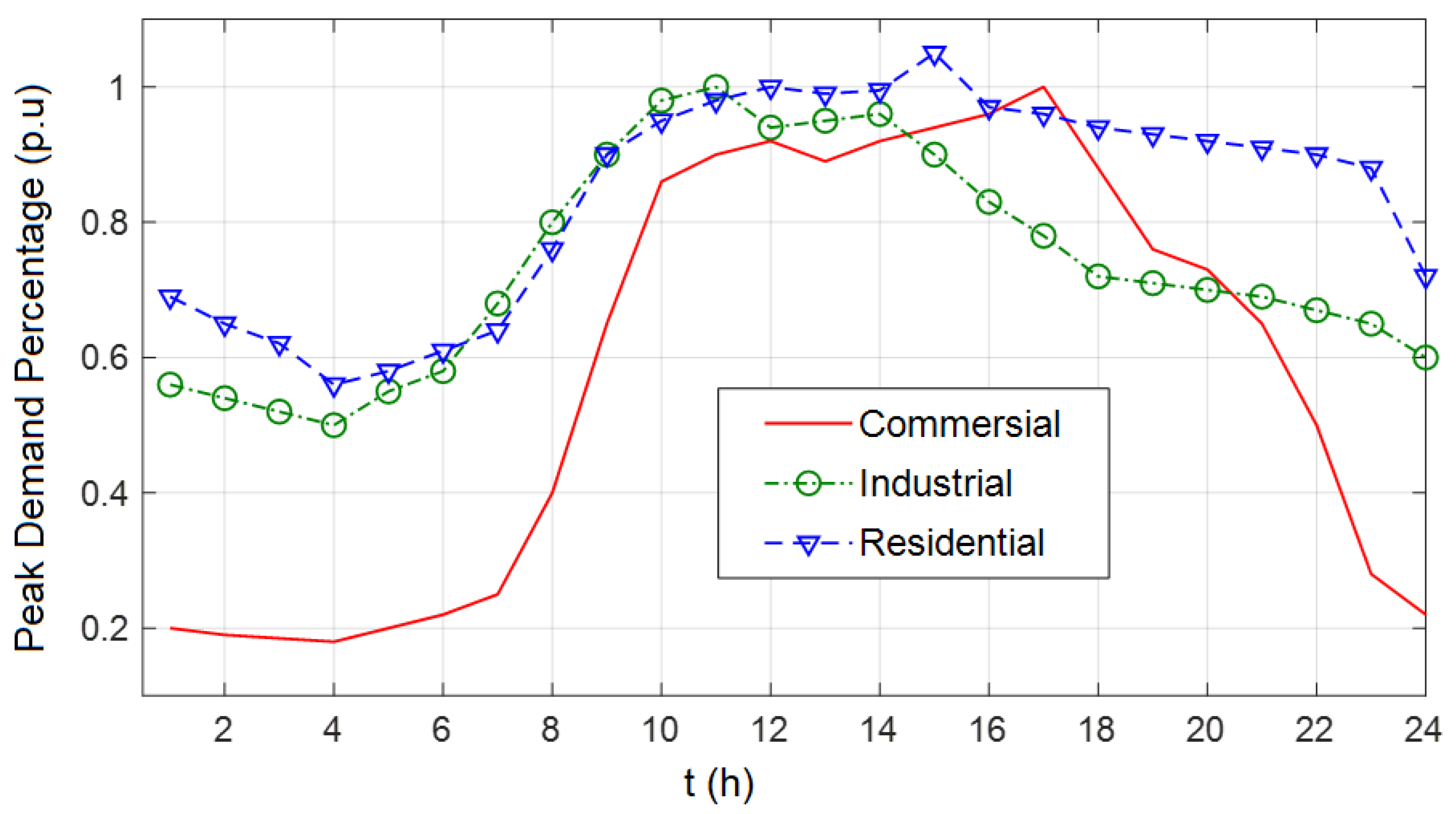
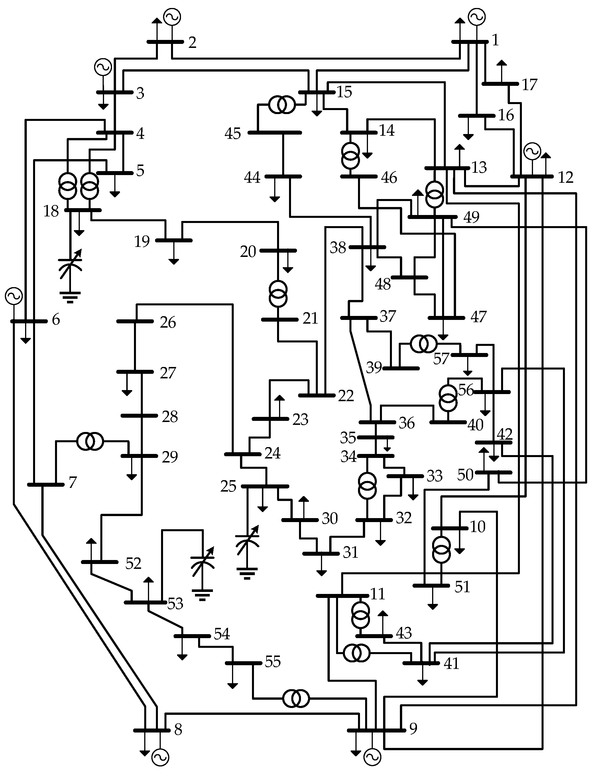
4.1. Description of the Test Systems

Several simulations were performed on the IEEE 30-bus [63] and 57-bus test systems [64]. The IEEE 30-bus test system consists of 41 branches, 24 PQ buses, and 19 control variables; these include 6 generation units, 4 transformers, and 9 capacitors. The IEEE 57-bus test system consists of 80 branches, 50 PQ buses, and 25 control variables; these are 7 generation units, 15 transformers, and 3 capacitors. For both systems, a time horizon of 24 h is defined, for which active and reactive power demands are established at each node. The per unit demand curve shown in Figure 3 illustrate the load curves of both systems. It should be noted that three types of users, namely residential, commercial, and industrial, were considered.

Table 2. Goal of power losses.

Test System	Power Losses (Base Case [MW])	Power Losses (Goal [MW])
IEEE-30 Bus	65.36	59.9
IEEE-57 Bus	241.7	219.5

presents the power losses for the base case and the goal aimed at for each test system. It is worth mentioning that this goal must be defined by the power system operator based on its knowledge of the system. In this case, the goal of power losses for each system was obtained through a sensitivity analysis.

One of the features that distinguish the proposed approach from other methods reported in the specialized literature is the handling of constraints. The sub-functions used to enforce constraints must be parameterized with several lambdas. In this case, the penalty factors (${\lambda }_v$, ${\lambda }_b$, ${\lambda }_{ct}$, ${\lambda }_{cc}$, ${\lambda }_{cr}$) for each of the sub-functions that make up the total fitness function are set to 0.05, except for ${\lambda }_l$ associated with the sub-function that enforces the maximum power flow through transmission lines which is set to 0.005, making this consideration less restrictive. These values of lambdas were established through sensitivity tests. Likewise, the cost per switching of transformer tap changers ($C{T}_k$) is defined as USD 6 per maneuver, and the cost per switching for capacitor banks ($C{C}_l$) is defined as USD 4 per maneuver. The maximum number of evaluations was set to 40,000, and 40 particles were used as initial candidate solutions.

The maximum number of daily operation allowed for the k-th transformer and $T{max}_{d,k}$ is established according to technical data. The daily limit is set to 114 maneuvers, taking into account 500,000 operations in 12 years [65]. As regards capacitor banks the maximum number of maneuvers recommended by the manufacturer is 100,000 in 20 years (to avoid premature maintenance interventions), which yields a maximum of 13 daily maneuvers [66].

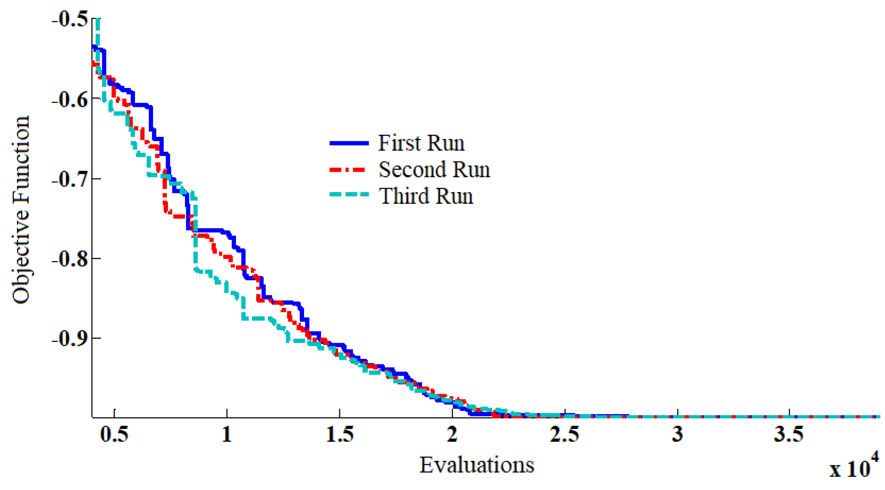
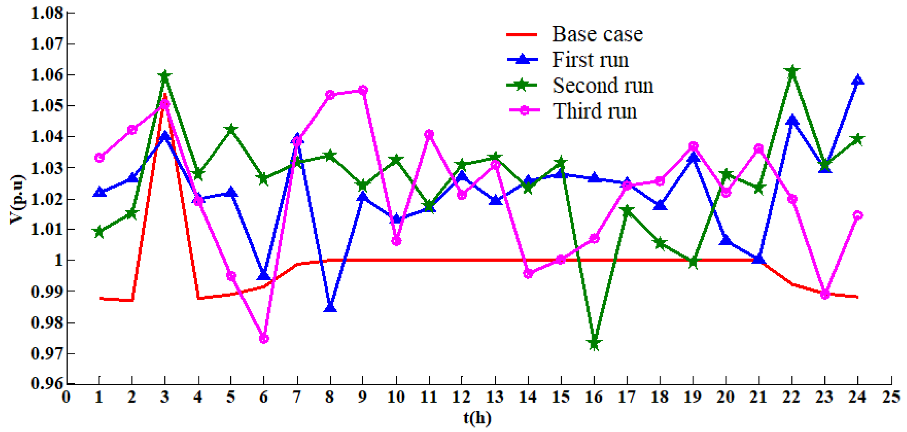
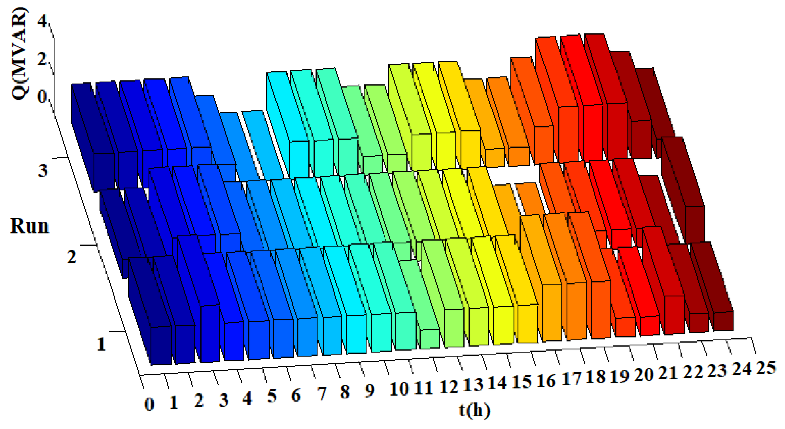
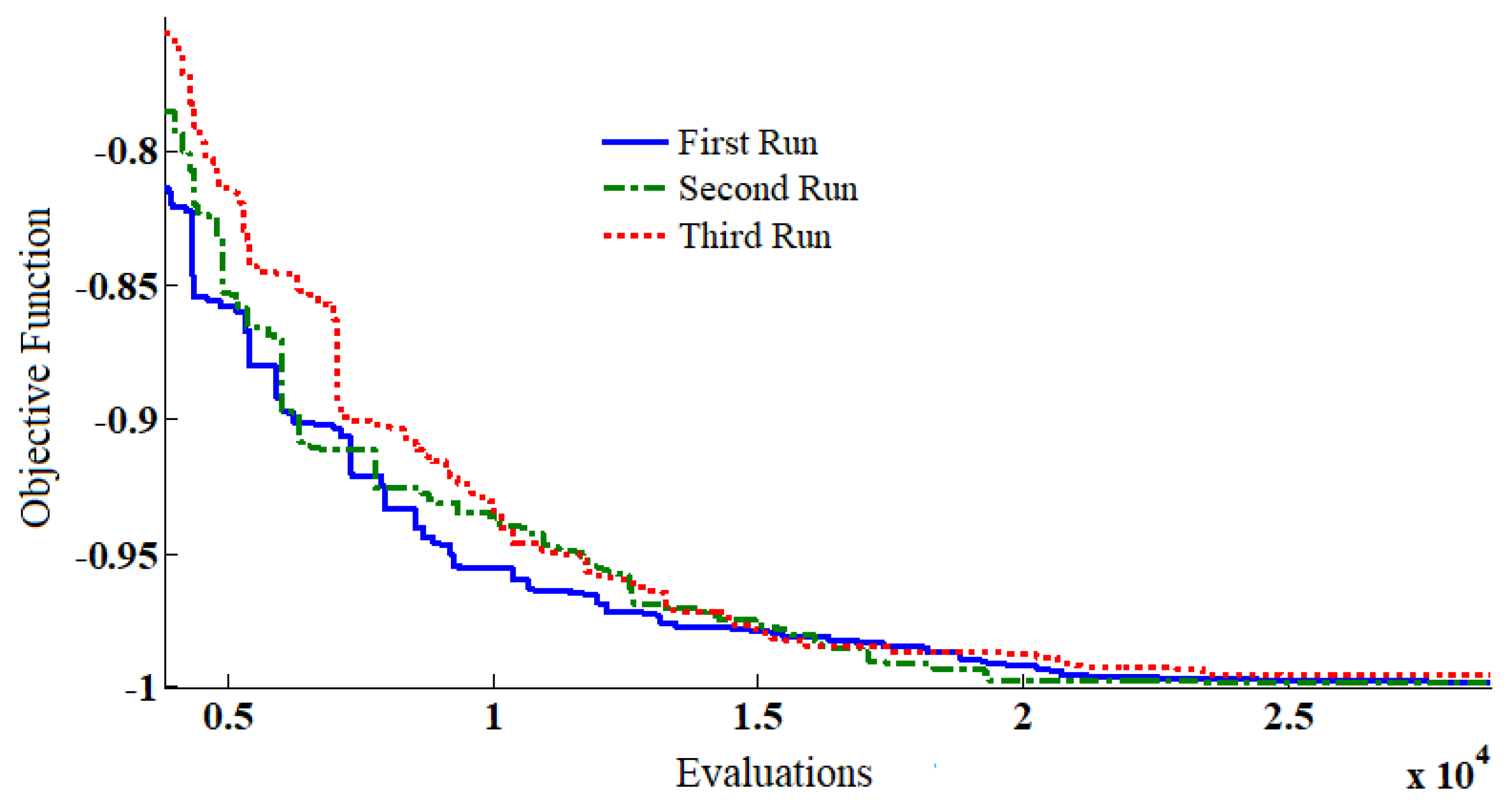
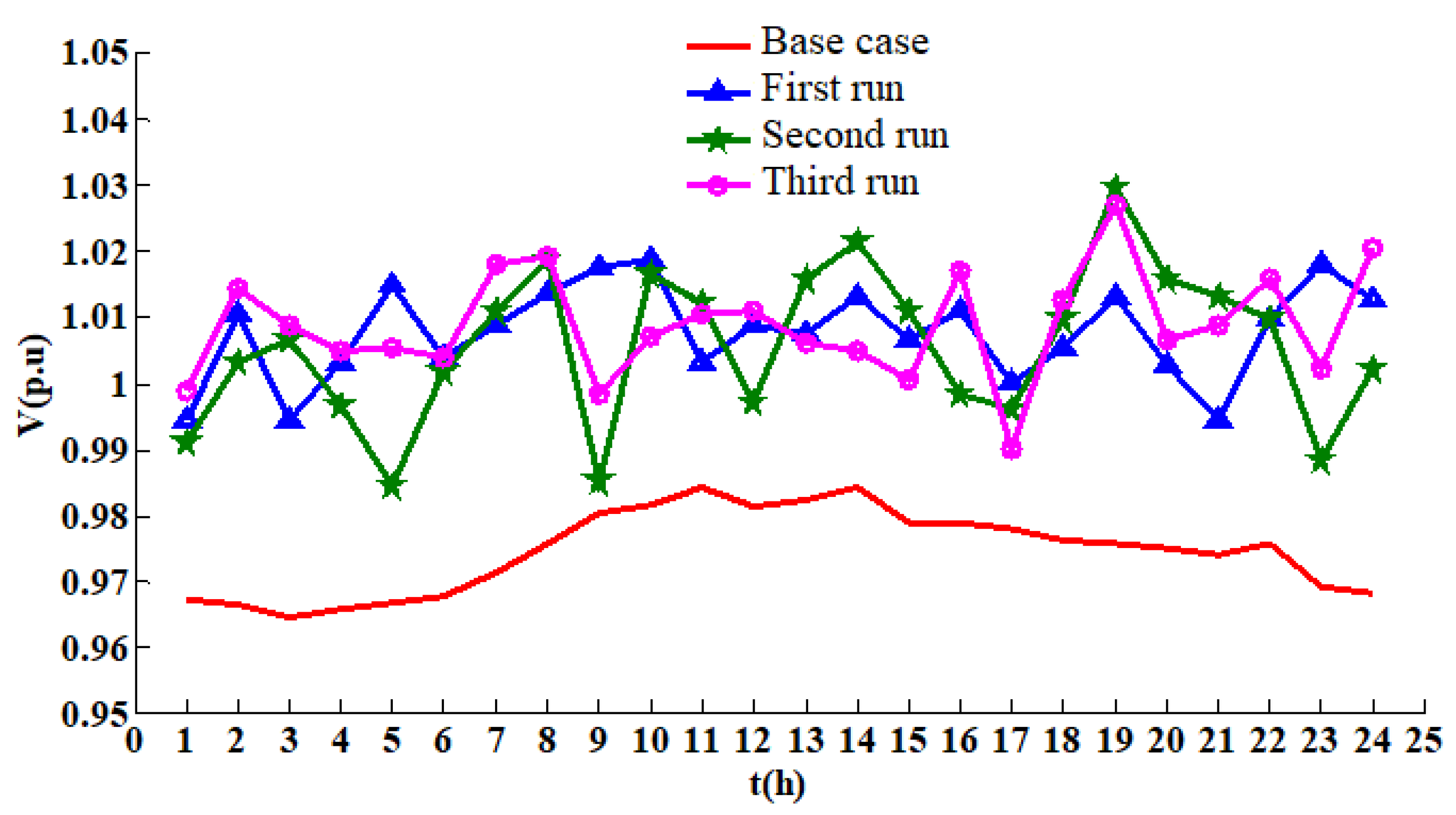
4.2. Results with the IEEE 30-Bus Test System

The IEEE 30-bus test system used in this paper is illustrated in Figure 4, to which 9 capacitor banks (each of 4 MVAr) proposed in [67] were incorporated. This results in 19 control variables which correspond to 6 controllable voltages at generation buses 1, 2, 22, 27, 23, and 13; 4 transformers with tap changers at branches 6–9, 6–10, 4–12, and 4–12; and 9 capacitor banks located at nodes 10, 12, 15, 17, 20, 21, 23, 24, and 29. In this case, the maximum demand is 181.73 MW in hour 14. Furthermore, voltage limits were set within 0.95–1.1 pu.

After running the MVMO algorithm, several feasible solutions were found for the MP-ORPD, which comply with the objective function and constraints. All tests were carried out on a laptop AMD Ryzen 7 with 20 G of RAM memory.

Table 3. Statistical results for 25 independent runs.

IEEE 30-Bus Test System	Power Losses (MW)	Time (s)
Best Solution	59.9128	3611
Worst Solution	59.9999	10,340
Mean	59.9838	7000
Standard Deviation	0.0186	1699

indicates the statistical results for 25 independent runs of the algorithm. The second column indicates the power loses achieved by the algorithm. It should be noted that despite the variety of solutions, most of them were significantly close to the goal of 59.9 MW of power losses set for the IEEE 30-bus test system. The third column indicates the processing time of the algorithm.

Figure 5 illustrates the convergence of the proposed algorithm for three independent runs. As the problem is set as a minimization the optimal solution is −1. Note that although 40,000 evaluations are set as the limit, the convergence is achieved at approximately 22,000 evaluations.

Figure 6 illustrates the voltage profile at generation bus 2 for three randomly selected runs of the algorithm. In this case, most voltage magnitudes are improved with respect to the base case. It is worth mentioning that the algorithm does not look for voltage improvement as such, but instead for a multi-period operation that guarantees power system limits and minimizes active power losses. In this case, all voltage magnitudes are within the permissible operating range.

Figure 7 depicts the voltage profile for load bus 22 (residential) for three random runs of the algorithm. An important improvement of voltage magnitude is observed for all runs. It should be noted that this improvement in voltage profile contributes to power loss reduction and also all voltages are within the allowed limits.

Figure 8 illustrates the hourly tap maneuvers for the transformer located at branch 6–10. It can be seen that there are no great changes in the maneuvers between consecutive hours. This minimization of maneuvers allows us to maintain the useful life of these equipment. A similar behavior was verified for the other transformers of the test system.

Figure 9 illustrates the variation of the reactive power injected by the capacitor bank located at bus 9. It was verified that there were no violations in the maximum number of maneuvers in any of the capacitor banks.

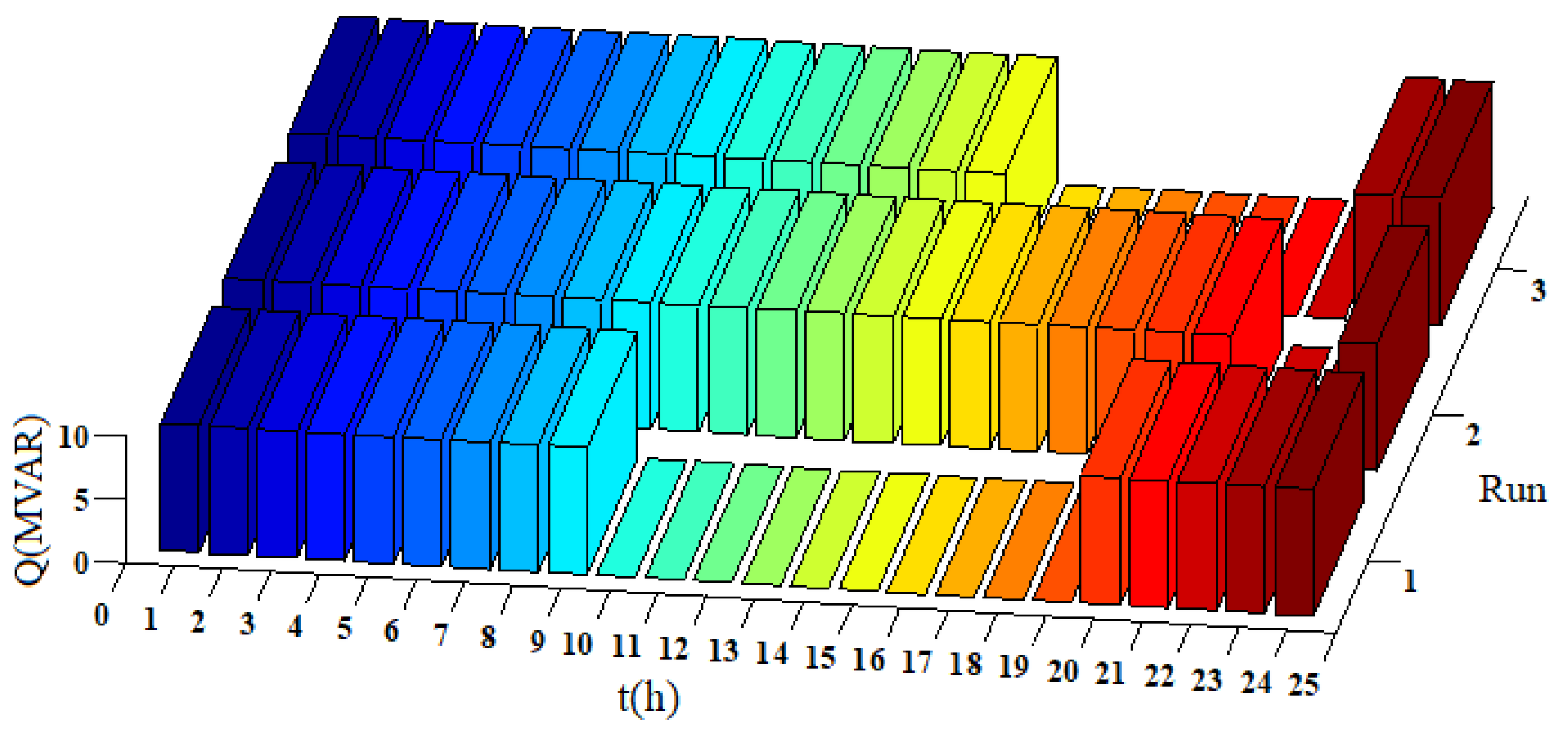
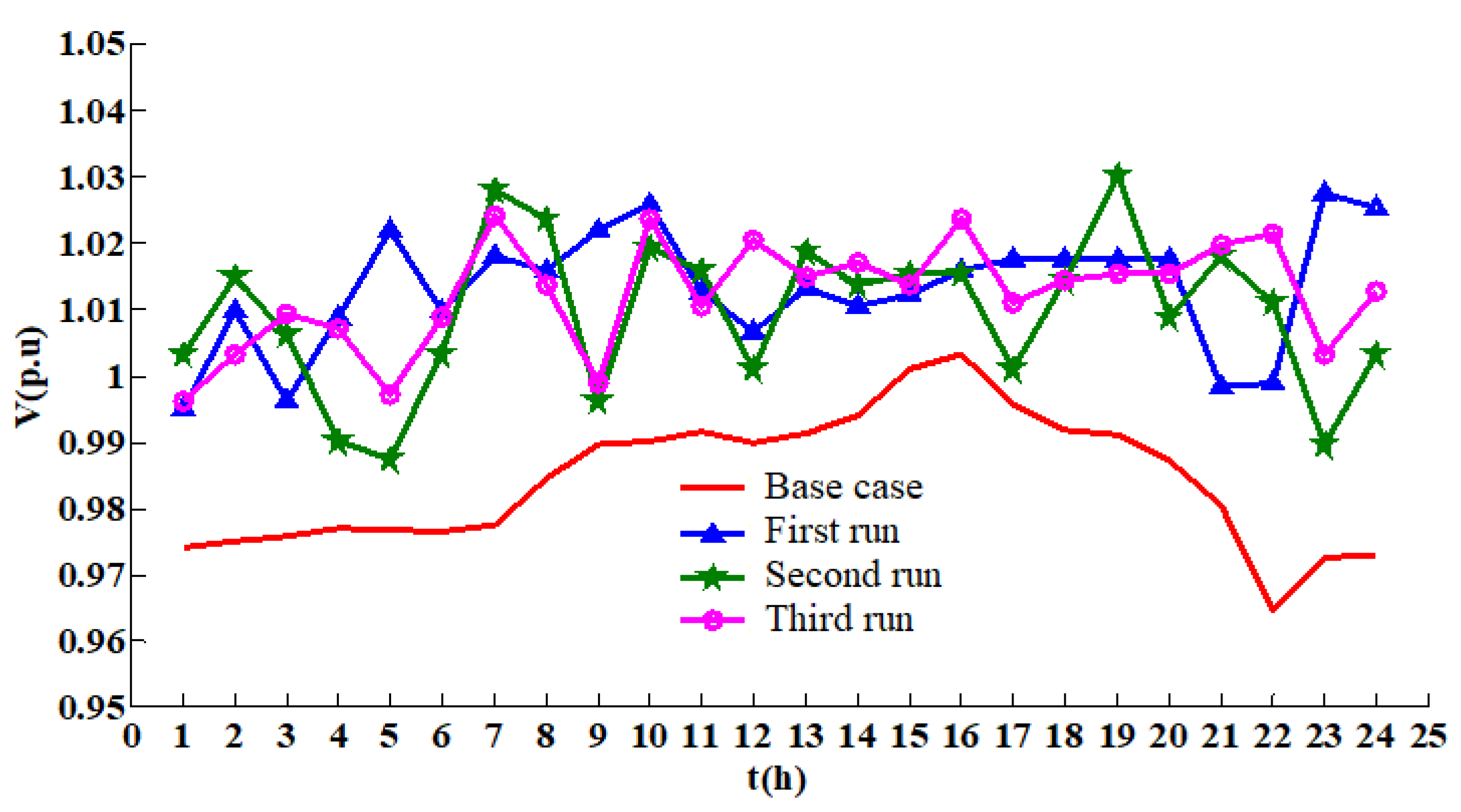
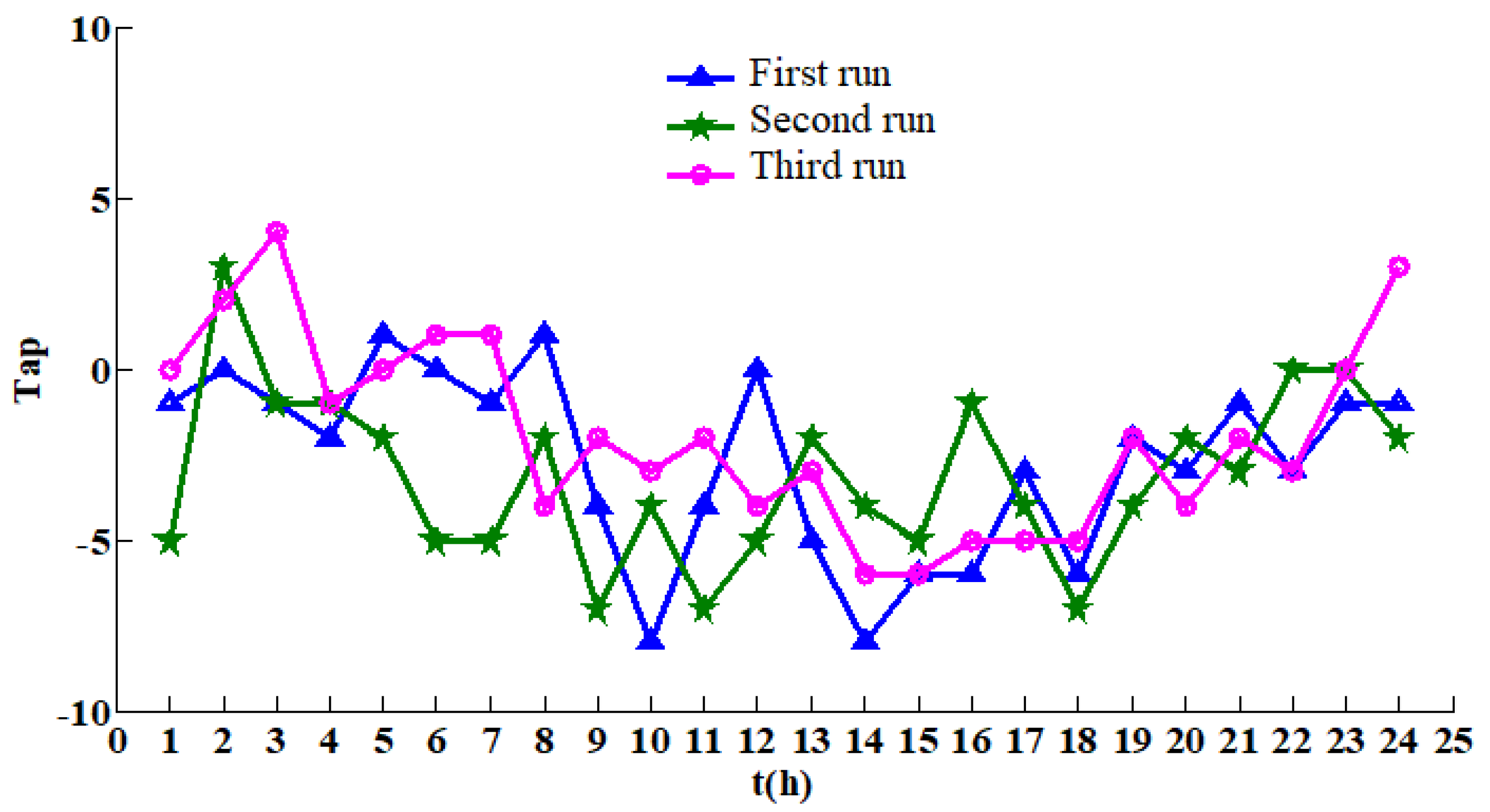
4.3. Results with the IEEE 57-Bus Test System

The IEEE 57-bus test system, illustrated in Figure 10, features 80 branches and 25 control variables: 7 generators with voltage control located at buses 1, 2, 3, 6, 8, 9, and 12; 15 on load tap changing transformers at branches 4–18 (2 transformers), 21–20, 24–26, 7–29, 34–32, 11–41, 15–45, 14–46, 10–51, 13–49, 11–43, 40–56, 39–57, and 9–55; and 3 capacitor banks located at nodes 18, 25, and 53.

Note that this system has more transformers than capacitor banks. For this reason, a single-step reactive power injection of 10 MVAr is considered for each capacitor bank.

After running the MVMO algorithm, several feasible solutions were found for the MP-ORPD, which comply with the objective function and constraints. All tests were carried out on a laptop AMD Ryzen 7 with 20 G of RAM memory.

Table 4. Statistical results for 25 independent runs.

IEEE 57-Bus Test System	Power Losses (MW)	Time (s)
Best Solution	219.8989	9922
Worst Solution	219.9972	20,619
Mean	219.9838	14,285
Standard Deviation	0.0256	2893

indicates the statistical results for 25 independent runs of the algorithm. The second column presents the power losses achieved by the algorithm. Note that despite the variety of solutions, most of them were significantly close to the goal of 219.5 MW of power losses set for the IEEE 57-bus test system. The third column indicates the computational time of the algorithm.

Figure 11 illustrates the convergence of the proposed algorithm for three independent runs. The maximum number of evaluations was set to 40,000; nonetheless, it can be observed that the algorithm achieves convergence at approximately 25,000 evaluations.

Figure 12 illustrates the voltage setpoints of generator located at bus 3 for three independent runs of the algorithm. It should be noted that all voltage setpoints are higher than the ones given in the base case.

Figure 13 illustrates the voltage at load bus 9 for three runs of the algorithm. Note that the MP-ORPD allows having higher voltages in load buses; nonetheless none of them is out of the operative limits as indicted by the constraints.

Figure 14 illustrates the taps movement for the transformer located at branch 7–29. It should be noted that tap variations correspond to the limits previously established.

Figure 15 illustrates the reactive compensation provided by the capacitor bank located at bus 18. Note that this compensation is used almost all the periods in run 2; nonetheless, it is not used in certain periods of time for runs 1 and 3. It is worth mentioning that the compensation does not need to be fully active all the time, since it is used when needed, to comply with the constraints and objective function.

5. Conclusions

This paper presented a new mathematical model for the multi-period version of the ORPD problem. Besides traditional limits on voltage magnitudes and power flows, the proposed MP-ORPD model incorporates inter-temporal constraints related to the number of maneuvers of transformer taps and capacitor banks. Such constraints allow to maintain the useful life of these elements. A key aspect of the proposed modeling is the design of the objective function. This consists of a multiplication of sub-functions in which penalization due to constraint violations is included. The main advantage of this objective function is the fact that both feasibility and optimality are easily verified.

Several tests carried out on two benchmark power systems evidenced the effectiveness and applicability of the proposed approach. For both power systems is was found that the algorithm was capable of finding high-quality solutions within reasonable computational time.

The MVMO algorithm proved to be an effective tool for solving the proposed MP-ORPD model. This technique presented adequate convergence as evidenced in the results. It is worth mentioning that for all the solutions found by the MVMO, the operative constraints and goal on power losses were achieved. Furthermore, there are notable improvements in the voltage profiles and in the reduction in transformer taps and capacitor bank maneuvers.

Although the MVMO proved to be an effective tool for solving the MP-ORPD, its main limitation lies in the high computational time required to find a solution. Nonetheless, such drawback is shared by all metaheuristic techniques. It is worth mentioning that the computational time is not a major inconvenience, since the MP-ORPD as proposed in this paper is not envisaged to be carried out online. A solution to the this issue and a future work is to explore parallel computation alternatives to reduce the computational time of the MP-ORPD.

References

1. Hassan, M.H.; Kamel, S.; El-Dabah, M.A.; Khurshaid, T.; Domínguez-García, J.L. Optimal Reactive Power Dispatch with Time-Varying Demand and Renewable Energy Uncertainty Using Rao-3 Algorithm. IEEE Access 2021, 9, 23264–23283. [Google Scholar] [CrossRef]
2. Mugemanyi, S.; Qu, Z.; Rugema, F.X.; Dong, Y.; Bananeza, C.; Wang, L. Optimal Reactive Power Dispatch Using Chaotic Bat Algorithm. IEEE Access 2020, 8, 65830–65867. [Google Scholar] [CrossRef]
3. Constante, F.S.G.; López, J.C.; Rider, M.J. Optimal Reactive Power Dispatch With Discrete Controllers Using a Branch-and-Bound Algorithm: A Semidefinite Relaxation Approach. IEEE Trans. Power Syst. 2021, 36, 4539–4550. [Google Scholar] [CrossRef]
4. Deeb, N.I.; Shahidehpour, S.M. An Efficient Technique for Reactive Power Dispatch Using a Revised Linear Programming Approach. Electr. Power Syst. Res. 1988, 15, 121–134. [Google Scholar] [CrossRef]
5. Sachdeva, S.S.; Billinton, R. Optimum Network Var Planning by Nonlinear Programming. IEEE Trans. Power Appar. Syst. 1973, PAS-92, 1217–1225. [Google Scholar] [CrossRef]
6. Grudinin, N. Reactive power optimization using successive quadratic programming method. IEEE Trans. Power Syst. 1998, 13, 1219–1225. [Google Scholar] [CrossRef]
7. Quintana, V.; Santos-Nieto, M. Reactive-power dispatch by successive quadratic programming. IEEE Trans. Energy Convers. 1989, 4, 425–435. [Google Scholar] [CrossRef]
8. Granville, S. Optimal reactive dispatch through interior point methods. IEEE Trans. Power Syst. 1994, 9, 136–146. [Google Scholar] [CrossRef]
9. Bjelogrlic, M.; Calovic, M.; Ristanovic, P.; Babic, B. Application of Newton’s optimal power flow in voltage/reactive power control. IEEE Trans. Power Syst. 1990, 5, 1447–1454. [Google Scholar] [CrossRef]
10. Zhu, J.; Xiong, X. Optimal reactive power control using modified interior point method. Electr. Power Syst. Res. 2003, 66, 187–192. [Google Scholar] [CrossRef]
11. Yu, D.C.; Fagan, J.E.; Foote, B.; Aly, A.A. An optimal load flow study by the generalized reduced gradient approach. Electr. Power Syst. Res. 1986, 10, 47–53. [Google Scholar] [CrossRef]
12. Deeb, N.; Shahidehpour, S. Linear reactive power optimization in a large power network using the decomposition approach. IEEE Trans. Power Syst. 1990, 5, 428–438. [Google Scholar] [CrossRef]
13. López-Lezama, J.M.; Cortina-Gómez, J.; Muñoz-Galeano, N. Assessment of the Electric Grid Interdiction Problem using a nonlinear modeling approach. Electr. Power Syst. Res. 2017, 144, 243–254. [Google Scholar] [CrossRef]
14. Saldarriaga-Zuluaga, S.D.; López-Lezama, J.M.; Muñoz-Galeano, N. Adaptive protection coordination scheme in microgrids using directional over-current relays with non-standard characteristics. Heliyon 2021, 7, e06665. [Google Scholar] [CrossRef] [PubMed]
15. Agudelo, L.; López-Lezama, J.M.; Muñoz-Galeano, N. Vulnerability assessment of power systems to intentional attacks using a specialized genetic algorithm. Dyna 2015, 82, 78–84. [Google Scholar] [CrossRef]
16. Niu, M.; Xu, N.Z.; Dong, H.N.; Ge, Y.Y.; Liu, Y.T.; Ngin, H.T. Adaptive Range Composite Differential Evolution for Fast Optimal Reactive Power Dispatch. IEEE Access 2021, 9, 20117–20126. [Google Scholar] [CrossRef]
17. Subbaraj, P.; Rajnarayanan, P. Optimal reactive power dispatch using self-adaptive real coded genetic algorithm. Electr. Power Syst. Res. 2009, 79, 374–381. [Google Scholar] [CrossRef]
18. Zhang, M.; Li, Y. Multi-Objective Optimal Reactive Power Dispatch of Power Systems by Combining Classification-Based Multi-Objective Evolutionary Algorithm and Integrated Decision Making. IEEE Access 2020, 8, 38198–38209. [Google Scholar] [CrossRef]
19. Zhihuan, L.; Yinhong, L.; Xianzhong, D. Non-dominated sorting genetic algorithm-II for robust multi-objective optimal reactive power dispatch. IET Gener. Transm. Distrib. 2010, 4, 1000–1008. [Google Scholar] [CrossRef]
20. Bhattacharyya, B.; Gupta, V. Fuzzy based evolutionary algorithm for reactive power optimization with FACTS devices. Int. J. Electr. Power Energy Syst. 2014, 61, 39–47. [Google Scholar] [CrossRef]
21. Jamal, R.; Men, B.; Khan, N.H. A Novel Nature Inspired Meta-Heuristic Optimization Approach of GWO Optimizer for Optimal Reactive Power Dispatch Problems. IEEE Access 2020, 8, 202596–202610. [Google Scholar] [CrossRef]
22. Yoshida, H.; Kawata, K.; Fukuyama, Y.; Takayama, S.; Nakanishi, Y. A particle swarm optimization for reactive power and voltage control considering voltage security assessment. IEEE Trans. Power Syst. 2000, 15, 1232–1239. [Google Scholar] [CrossRef] [Green Version]
23. Martinez-Rojas, M.; Sumper, A.; Bellmunt, O.; Sudria-Andreu, A. Reactive power dispatch in wind farms using particle swarm optimization technique and feasible solutions search. Appl. Energy 2011, 88, 4678–4686. [Google Scholar] [CrossRef]
24. Liang, R.H.; Wang, J.C.; Chen, Y.T.; Tseng, W.T. An enhanced firefly algorithm to multi-objective optimal active/reactive power dispatch with uncertainties consideration. Int. J. Electr. Power Energy Syst. 2015, 64, 1088–1097. [Google Scholar] [CrossRef]
25. De, M.; Goswami, S.K. Optimal Reactive Power Procurement With Voltage Stability Consideration in Deregulated Power System. IEEE Trans. Power Syst. 2014, 29, 2078–2086. [Google Scholar] [CrossRef]
26. Malakar, T.; Goswami, S. Active and reactive dispatch with minimum control movements. Int. J. Electr. Power Energy Syst. 2013, 44, 78–87. [Google Scholar] [CrossRef]
27. Duman, S.; Sonmez, Y.; Guvenc, U.; Yorukeren, N. Optimal reactive power dispatch using a gravitational search algorithm. IET Gener. Transm. Distrib. 2012, 6, 563. [Google Scholar] [CrossRef]
28. Niknam, T.; Narimani, M.R.; Azizipanah-Abarghooee, R.; Bahmani-Firouzi, B. Multiobjective Optimal Reactive Power Dispatch and Voltage Control: A New Opposition-Based Self-Adaptive Modified Gravitational Search Algorithm. IEEE Syst. J. 2013, 7, 742–753. [Google Scholar] [CrossRef]
29. Khazali, A.; Kalantar, M. Optimal reactive power dispatch based on harmony search algorithm. Int. J. Electr. Power Energy Syst. 2011, 33, 684–692. [Google Scholar] [CrossRef]
30. Kn, L.; Reddy, B.; Kalavathi, M. A New charged system Search for Solving Optimal Reactive Power Dispatch Problem. Int. J. Comput. 2014, 14, 22–40. [Google Scholar]
31. Yan, W.; Liu, F.; Chung, C.; Wong, K. A hybrid genetic algorithm-interior point method for optimal reactive power flow. IEEE Trans. Power Syst. 2006, 21, 1163–1169. [Google Scholar] [CrossRef] [Green Version]
32. Huang, C.M.; Huang, Y.C. Combined Differential Evolution Algorithm and Ant System for Optimal Reactive Power Dispatch. Energy Procedia 2012, 14, 1238–1243. [Google Scholar] [CrossRef] [Green Version]
33. Laouafi, F.; Boukadoum, A.; Leulmi, S. Reactive Power Dispatch with Hybrid Formulation: Particle Swarm Optimization and Improved Genetic Algorithms with Real Coding. Int. Rev. Electr. Eng. 2010, 5, 601–607. [Google Scholar]
34. Jamal, R.; Men, B.; Khan, N.H.; Raja, M.A.Z.; Muhammad, Y. Application of Shannon Entropy Implementation Into a Novel Fractional Particle Swarm Optimization Gravitational Search Algorithm (FPSOGSA) for Optimal Reactive Power Dispatch Problem. IEEE Access 2021, 9, 2715–2733. [Google Scholar] [CrossRef]
35. Kanna, B.; Singh, S.N. Towards reactive power dispatch within a wind farm using hybrid PSO. Int. J. Electr. Power Energy Syst. 2015, 69, 232–240. [Google Scholar] [CrossRef]
36. Vlachogiannis, J.; Lee, K. A Comparative Study on Particle Swarm Optimization for Optimal Steady-State Performance of Power Systems. IEEE Trans. Power Syst. 2006, 21, 1718–1728. [Google Scholar] [CrossRef] [Green Version]
37. Srivastava, L.; Singh, H. Hybrid multi-swarm particle swarm optimisation based multi-objective reactive power dispatch. IET Gener. Transm. Distrib. 2015, 9, 727–739. [Google Scholar] [CrossRef]
38. Gutierrez Rojas, D.; Lopez Lezama, J.; Villa, W. Metaheuristic Techniques Applied to the Optimal Reactive Power Dispatch: A Review. IEEE Latin Am. Trans. 2016, 14, 2253–2263. [Google Scholar] [CrossRef]
39. Marín-Cano, C.C.; Sierra-Aguilar, J.E.; López-Lezama, J.M.; Jaramillo-Duque, A.; Villegas, J.G. A Novel Strategy to Reduce Computational Burden of the Stochastic Security Constrained Unit Commitment Problem. Energies 2020, 13, 3777. [Google Scholar] [CrossRef]
40. Yang, B.; Cao, X.; Cai, Z.; Yang, T.; Chen, D.; Gao, X.; Zhang, J. Unit Commitment Comprehensive Optimal Model Considering the Cost of Wind Power Curtailment and Deep Peak Regulation of Thermal Unit. IEEE Access 2020, 8, 71318–71325. [Google Scholar] [CrossRef]
41. Naghdalian, S.; Amraee, T.; Kamali, S.; Capitanescu, F. Stochastic Network-Constrained Unit Commitment to Determine Flexible Ramp Reserve for Handling Wind Power and Demand Uncertainties. IEEE Trans. Ind. Inform. 2020, 16, 4580–4591. [Google Scholar] [CrossRef]
42. Sierra-Aguilar, J.E.; Marín-Cano, C.C.; López-Lezama, J.M.; Jaramillo-Duque, A.; Villegas, J.G. A New Affinely Adjustable Robust Model for Security Constrained Unit Commitment under Uncertainty. Appl. Sci. 2021, 11, 3987. [Google Scholar] [CrossRef]
43. Zhao, J.; Ju, L.; Dai, Z.; Chen, G. Voltage stability constrained dynamic optimal reactive power flow based on branch-bound and primal–dual interior point method. Int. J. Electr. Power Energy Syst. 2015, 73, 601–607. [Google Scholar] [CrossRef]
44. Liu, M.B.; Canizares, C.A.; Huang, W. Reactive Power and Voltage Control in Distribution Systems With Limited Switching Operations. IEEE Trans. Power Syst. 2009, 24, 889–899. [Google Scholar] [CrossRef]
45. Agalgaonkar, Y.P.; Pal, B.C.; Jabr, R.A. Distribution Voltage Control Considering the Impact of PV Generation on Tap Changers and Autonomous Regulators. IEEE Trans. Power Syst. 2014, 29, 182–192. [Google Scholar] [CrossRef] [Green Version]
46. Hu, Z.; Wang, X.; Chen, H.; Taylor, G. Volt/VAR control in distribution systems using a time-interval based approach. IEE Proc. Gener. Transm. Distrib. 2003, 150, 548–554. [Google Scholar] [CrossRef]
47. Sharma, A.; Jain, S.K. Day-ahead optimal reactive power ancillary service procurement under dynamic multi-objective framework in wind integrated deregulated power system. Energy 2021, 223, 120028. [Google Scholar] [CrossRef]
48. Kim, Y.J.; Ahn, S.J.; Hwang, P.I.; Pyo, G.C.; Moon, S.I. Coordinated Control of a DG and Voltage Control Devices Using a Dynamic Programming Algorithm. IEEE Trans. Power Syst. 2013, 28, 42–51. [Google Scholar] [CrossRef]
49. Huang, J.; Li, Z.; Wu, Q. Fully decentralized multiarea reactive power optimization considering practical regulation constraints of devices. Int. J. Electr. Power Energy Syst. 2019, 105, 351–364. [Google Scholar] [CrossRef]
50. Morán-Burgos, J.A.; Sierra-Aguilar, J.E.; Villa-Acevedo, W.M.; López-Lezama, J.M. A Multi-Period Optimal Reactive Power Dispatch Approach Considering Multiple Operative Goals. Appl. Sci. 2021, 11, 8535. [Google Scholar] [CrossRef]
51. Ahmadi, H.; Martí, J.R.; Dommel, H.W. A Framework for Volt-VAR Optimization in Distribution Systems. IEEE Trans. Smart Grid 2015, 6, 1473–1483. [Google Scholar] [CrossRef]
52. Zhang, Y.-J.; Ren, Z. Optimal reactive power dispatch considering costs of adjusting the control devices. IEEE Trans. Power Syst. 2005, 20, 1349–1356. [Google Scholar] [CrossRef]
53. Yang, W.; Chen, L.; Deng, Z.; Xu, X.; Zhou, C. A multi-period scheduling strategy for ADN considering the reactive power adjustment ability of DES. Int. J. Electr. Power Energy Syst. 2020, 121, 106095. [Google Scholar] [CrossRef]
54. Ibrahim, T.M.S.; De Rubira, T.T.; Del Rosso, A.; Patel, M.; Guggilam, S.; Mohamed, A. Alternating Optimization Approach for Voltage-Secure Multi-Period Optimal Reactive Power Dispatch. IEEE Trans. Power Syst. 2021, 1. [Google Scholar] [CrossRef]
55. Villa-Acevedo, W.M.; López-Lezama, J.M.; Valencia-Velásquez, J.A. A Novel Constraint Handling Approach for the Optimal Reactive Power Dispatch Problem. Energies 2018, 11, 2352. [Google Scholar] [CrossRef] [Green Version]
56. Londoño, D.C.; Villa-Acevedo, W.M.; López-Lezama, J.M. Assessment of Metaheuristic Techniques Applied to the Optimal Reactive Power Dispatch. In Proceedings of the Applied Computer Sciences in Engineering; Communications in Computer and Information Science; Springer International Publishing: Cham, Switzerland, 2019; pp. 250–262. [Google Scholar] [CrossRef]
57. Nakawiro, W.; Erlich, I.; Rueda, J.L. A novel optimization algorithm for optimal reactive power dispatch: A comparative study. In Proceedings of the 2011 4th International Conference on Electric Utility Deregulation and Restructuring and Power Technologies (DRPT), Weihai, China, 6–9 July 2011; pp. 1555–1561. [Google Scholar] [CrossRef]
58. Rueda, J.L.; Erlich, I. Optimal dispatch of reactive power sources by using MVMO optimization. In Proceedings of the 2013 IEEE Computational Intelligence Applications in Smart Grid (CIASG), Singapore, 16–19 April 2013; pp. 29–36. [Google Scholar] [CrossRef]
59. Erlich, I. Mean-Variance Mapping Optimization Algorithm Home Page. Available online: https://www.uni-due.de/mvmo/ (accessed on 10 November 2020).
60. Erlich, I.; Venayagamoorthy, G.K.; Worawat, N. A Mean-Variance Optimization algorithm. In Proceedings of the IEEE Congress on Evolutionary Computation, Barcelona, Spain, 18–23 July 2010; pp. 1–6. [Google Scholar] [CrossRef]
61. Cepeda, J.C.; Rueda, J.L.; Erlich, I. Identification of dynamic equivalents based on heuristic optimization for smart grid applications. In Proceedings of the 2012 IEEE Congress on Evolutionary Computation, Brisbane, Australia, 10–15 June 2012; pp. 1–8. [Google Scholar] [CrossRef] [Green Version]
62. Rueda, J.L.; Erlich, I. Evaluation of the mean-variance mapping optimization for solving multimodal problems. In Proceedings of the 2013 IEEE Symposium on Swarm Intelligence (SIS), Singapore, 16–19 April 2013; pp. 7–14. [Google Scholar] [CrossRef]
63. University of Illinois. ICSEG Power Case 1—IEEE 30 Bus Systems. Available online: https://uofi.app.box.com/s/frjqsg9vpe6dvv7ufodd (accessed on 10 November 2020).
64. University of Washington. Power Systems Test Case Archive—UWEE. Available online: https://labs.ece.uw.edu/pstca/ (accessed on 10 November 2020).
65. ABB. Cambiador de Tomas en Carga, Tipo UBB Guía de Mantenimiento; Technical Report; 1ZSE 5492-127 es, Rev. 5; ABB: Ludvika, Suecia, 2005. [Google Scholar]
66. ABB. Interruptores de Tanque Vivo; Guia de Usuario Edición 4, 2008-10; ABB: Ludvika, Suecia, 2008. [Google Scholar]
67. Ela, A.A.E.; Abido, M.; Spea, S. Differential evolution algorithm for optimal reactive power dispatch. Electr. Power Syst. Res. 2011, 81, 458–464. [Google Scholar] [CrossRef]
Figure 1. (a) Power flow limits of branch j at time t; (b) voltage limits for bus i at time t; and (c) active power loss limit.
Computers 11 00048 g001
Figure 2. Flowchart of the swarm MVMO [58].
Computers 11 00048 g002
Figure 3. Daily hourly demand curves according to the type of users.
Computers 11 00048 g003
Figure 4. IEEE 30-bus test system.
Computers 11 00048 g004
Figure 5. Convergence of the MVMO algorithm for the IEEE 30-bus test system.
Computers 11 00048 g005
Figure 6. Voltage profile at generation bus 2 for several runs of the algorithm.
Computers 11 00048 g006
Figure 7. Voltage profile at load bus 22 (residential) for several runs of the algorithm.
Computers 11 00048 g007
Figure 8. Hourly variation of transformer taps located in branch 6–10 for the IEEE 30-bus test system.
Computers 11 00048 g008
Figure 9. Reactive power variation of capacitor bank located at node 9 (IEEE 30-bus test system).
Computers 11 00048 g009
Figure 10. IEEE 57-bus test system.
Computers 11 00048 g010
Figure 11. Convergence of the MVMO algorithm for the IEEE 57-bus test system.
Computers 11 00048 g011
Figure 12. Voltage set-points of generator at bus 3 for different runs of the algorithm (IEEE 57-bus test system).
Computers 11 00048 g012
Figure 13. Voltage profile at load bus 9 for different runs of the algorithm (IEEE 57-bus test system).
Computers 11 00048 g013
Figure 14. Voltage profile at load bus 9 for different runs of the algorithm (IEEE 57-bus test system).
Computers 11 00048 g014
Figure 15. Dispatch of the capacitive compensation located at bus 18 (IEEE 57-bus test system).
Computers 11 00048 g015