Article

Vehicle Auto-Classification Using Machine Learning Algorithms Based on Seismic Fingerprinting

by
Ahmad Bahaa Ahmad
1,2,
Hakim Saibi
3,
Abdelkader Nasreddine Belkacem
4 and
Takeshi Tsuji
1,2,5,*
1
Department of Earth Resources Engineering, Kyushu University, 744 Motooka, Nishi-ku, Fukuoka 819-0395, Japan
2
School of Engineering, The University of Tokyo, 7-3-1 Hongo Bunkyo-ku, Tokyo 113-8656, Japan
3
Geosciences Department, College of Science, United Arab Emirates University, Al-Ain 15551, United Arab Emirates
4
Department of Computer and Network Engineering, United Arab Emirates University, Al-Ain 15551, United Arab Emirates
5
International Institute for Carbon-Neutral Energy Research (I2CNER), Kyushu University, 744 Motooka, Nishi-ku, Fukuoka 819-0395, Japan
*
Author to whom correspondence should be addressed.
Computers 2022, 11(10), 148; https://doi.org/10.3390/computers11100148
Submission received: 13 August 2022 / Revised: 24 September 2022 / Accepted: 27 September 2022 / Published: 30 September 2022
(This article belongs to the Special Issue Machine Learning for Traffic Modeling and Prediction)

Abstract

:
Most vehicle classification systems now use data from images or videos. However, these approaches violate drivers’ privacy and reveal their identities. Due to various disruptions, detecting automobiles using seismic ambient noise signals is challenging. This study uses seismic surface waves to compare time series data between different vehicle types. We applied various artificial intelligence approaches using raw data from three different vehicle sizes (Bus/Truck, Car, and Motorcycle) and background noise. By using vertical component seismic data, this study compares the decoding abilities of Logistic Regression, Support Vector Machine, and Naïve Bayes (NB) approaches to determine the class of automobiles. The Multiclass classifiers were trained on 4185 samples and tested on 1395 randomly chosen from actual and synthetic data sets. Additionally, we used the convolutional neural network approach as a baseline to assess the effectiveness of machine learning (ML) methods. The NB method showed relatively high classification accuracy during training for the three multiclass classification situations. Overall, we investigate an ML-based decoding technique that can be used for security and traffic analysis across large geographic areas without endangering driver privacy and is more effective and economical than conventional methods.

1. Introduction

Many nations have made significant investments in traffic monitoring systems [1], which gather and analyze traffic data to produce statistics concerning the number of vehicles on the road and their usage trends over time. Governments can use these figures to plan road upkeep and estimate future transportation demands. A crucial aspect in predicting noise levels and road damage is determining the size of vehicles—according to the Traffic Monitoring Guide report released by the Federal Highway Administration in the United States [2], a roadway’s geometry is designed based on the typical mix of vehicle types that utilize that route.
Vehicle detection systems use UpToDate sensing technology supported by machine learning (ML) approaches [3]. While modern systems achieve increasingly accurate vehicle classification, their features and requirements vary, including the types of sensors used, parameter settings, operational environments, and cost. Many traffic monitoring systems include methods for classifying vehicles based on eyesight, often cameras; these systems achieve high classification accuracy between 90 and 99% [4].
Although camera-based systems have a high degree of classification accuracy, other factors, such as weather and lighting, can impact their effectiveness. For example, an automobile can be fully or partially missed when a larger vehicle covers the camera’s view.
Additionally, such systems require significant infrastructure expenditure to cover the road network fully. Since many individuals do not feel comfortable being monitored by cameras, the associated privacy issues for vehicle occupants are also a significant issue. An inductive loop detector based on vehicles’ magnetic properties is one of the most commonly used traffic monitoring systems for vehicle recognition and categorization [5]. This loop detector technology is built on a coil of wire buried beneath the road that records changes in the amplitude, phase, and frequency of the magnetic profile signal when a vehicle passes over it [6]. The loop detector technique has been widely studied, with previous works demonstrating its high accuracy (99%) for classifying large vehicles, such as cars, trucks, and vans [7,8,9,10]. The accuracy of loop detector systems has been shown to be independent of vehicle speed [11].
Different sensor types have been utilized in other proposed privacy-preserving systems. When combining several sensor networks, magnetic sensors positioned in the middle of or adjacent roads can achieve vehicle classification accuracy levels of up to 96.4% [12,13,14]. In comparison, a combination of infrared and ultrasonic sensors can provide an accuracy of up to 99% [15]. In addition to the current methods, new approaches have been suggested for monitoring traffic congestion in metropolitan areas based on GPS, social media, and network data collected directly from vehicles [16,17,18,19,20]. Intelligent transportation systems have been developed using ML techniques, with detailed information on metropolitan area traffic patterns and travel patterns now available. However, compared to inductive loops and camera-based systems, most of the proposed methods are less accurate at categorization; in addition, these approaches may require specialized installations, such as loop detectors for public roadways [21].
A range of vibration-based vehicle classification techniques has been proposed to address this issue. Vehicles’ engine systems and the interaction of their tires with the road are the principal causes of vehicle vibrations [22,23,24], and the vehicle’s size significantly impacts these signals. Due to the impact of the underlying geology on the propagation of the seismic wave, it can be challenging to locate these signals. Due to the similar vibrations of most cars at frequencies around 20 Hz, identifying seismic signals from moving objects in real life remains challenging. However, these signals are less susceptible to wind noise due to passing through the ground, a factor that is advantageous for vehicle detection [25]. This study explores using artificial intelligence (AI) approaches to identify automobiles from seismic waves. AI has significantly improved voice recognition technologies, such as voice analysis, in the past ten years [26].
Additionally, AI has been applied to seismic event categorization [27,28,29,30]; thus, we consider this a promising approach to vehicle identification. In addition to its benefits for vehicle occupant privacy, AI seismic data-based traffic monitoring is also expected to achieve low power consumption and cost. Furthermore, seismic-based traffic monitoring can be implemented in remote and limited-access areas, and it can operate for extended periods (months) with minimum maintenance and power supply. Most seismic sensor systems are prepared for extreme environments, unlike camera-based systems. Moreover, the seismic system does not have a blind spot; it can cover a relatively large area and be hidden easily, making it suitable for security and border control purposes. A neural network was employed in a 2010 study to categorize automobiles based on seismic data [31], while another study published in 2019 only used seismic signatures [25]. In the latter work, a log-scaled frequency cepstral coefficient matrix was proposed to extract spectral information from vehicle seismic signals; this approach was able to classify objects with an accuracy of up to 91.39%. Both studies focused on large military vehicles; thus, these approaches cannot be directly applied to civilian cars. Additionally, neither technique can utilize seismic data without preprocessing or without the inclusion of additional data. Ahmad and Tsuji (2021) developed a seismometer-based traffic monitoring system using a convolutional neural network (CNN) [32]. However, this approach investigated only one specific branch of ML (the neural networks).
In this study, we used three distinct ML algorithms to classify the size of cars using seismic waves—Logistic Regression (LR), Support Vector Machine (SVM), and Naïve Bayes (NB). Previous studies have captured and categorized waveform data from various sources to investigate how effectively ML approaches can extract information from seismic waves; thus, we also contrast the findings of this investigation with the published CNN-based approach. This study will extend the investigation of using other ML algorithms to classify vehicles of different sizes based on their seismic signals. Although this study shares the same goal and data set as the previous study of Ahmad and Tsuji (2021) [32], it discusses the usage of more straightforward and linear methods such as LR to conclude if those methods are beneficial. Another difference between these methods (SVM, LR, and NB) and neural networks is that the idea of neural networks highly depends on optimized variables (weights/filters), making it relatively computationally consuming. The previous study investigated only a specific branch of ML, neural networks, and focused on the well-known architectures for voice recognition, such as CNN and RNN. To our knowledge, this is the first study to use Logistic Regression, Support Vector Machine, and Naïve Bayes to predict and classify vehicles using their ground motions.
This study highlights the ability of seismic surface ambient noise to carry more information than has been recognized, and we hope that the work presented here will inspire researchers to investigate more uses for seismic surface noise. This understanding can improve earthquake early warning systems, civil engineering, plant operations optimization, crime prevention, and even enhance hydrocarbon and water exploration by extracting hidden information.

2. Materials and Methods
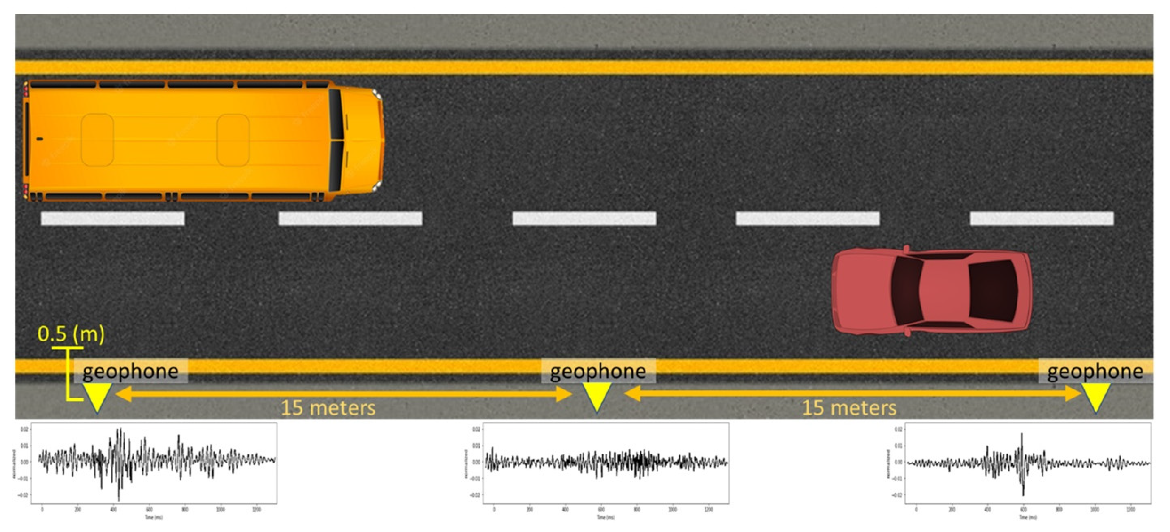
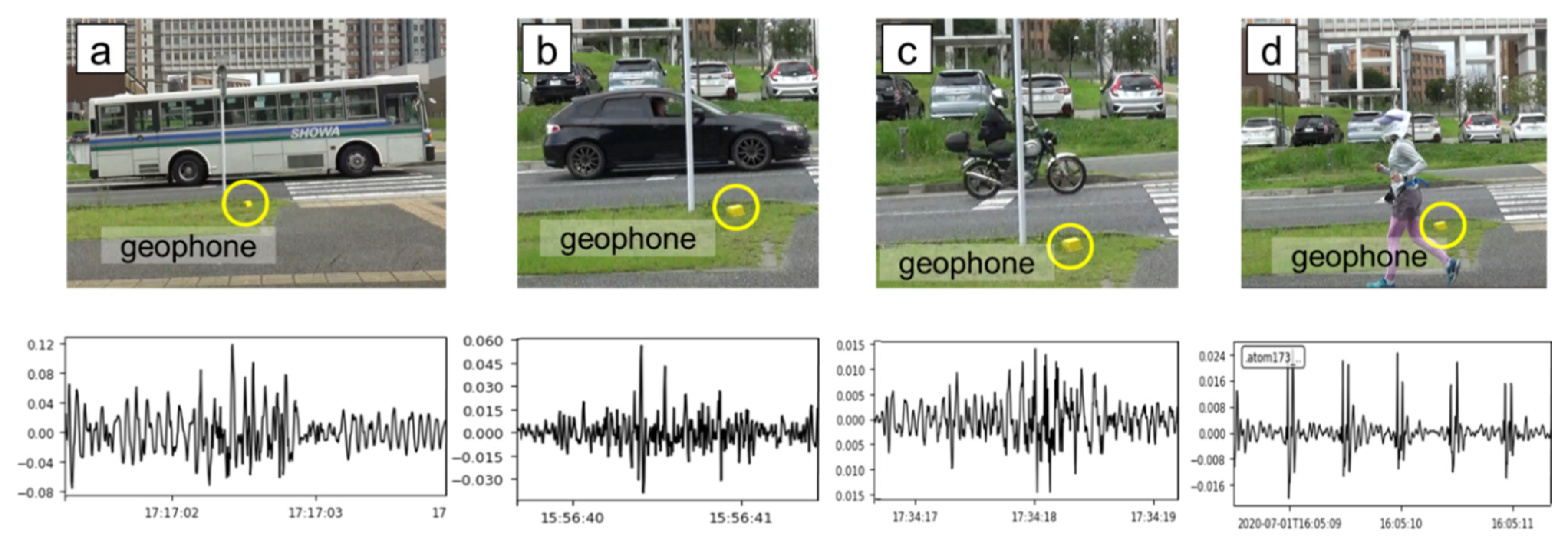
2.1. Data Set

For this investigation, we collected seismic vertical motion data for several cars using geophones at Kyushu University in July 2020. The geophones were set up at three sites, each 15 m apart and 0.5 m from the road. Vibrations in the vertical direction were captured at a 250 Hz sampling rate. We categorize vehicles as large (e.g., buses and trucks), medium (e.g., passenger cars), and small (e.g., motorcycles and scooters) size. Figure 1 shows the configuration of the seismic sensors used in the survey.
We used video records as a visual guide to preparing the events/vehicles catalog. The video camera and geophones were synchronized to a GPS clock to ensure accuracy in data preparation. However, the video/images were not used as data input for the algorithms. When an automobile was near the geophone, each event (i.e., the passage of a vehicle) lasted 2–3 s.
We calculated the automobiles’ speeds based on the signals from three stations. Most of the cars measured in this experiment traveled between 25 and 35 km/h, with a top speed of 45 km/h. To prevent overfitting the models, we only included clear vehicle signals during the training phase, excluding any signals that had background noise or overlapped with other cars. The chosen occurrences were sliced from the record as 5-sec windows containing 1251 data points. The following mathematical formulations assume vibration data:
W = S(t)1, S(t)2, S(t)3, S(t)4, ……., S(t)n,
S is the geophone reading at time (t), which is 0.004 s (250 Hz) in this case, and n is the number of samples (1251) in the study case. This period was selected to ensure that the entire seismic waveform was fully included. We retrieved an average of 68 waveform windows per geophone station per vehicle class with a total of 612 events. To cover the noise as the fourth class in our data, we chose 318 representative waveform windows; strong winds, bicycles, pedestrians, trolley-pushing pedestrians, road maintenance, and general background noise represent several examples of noise sources. Thus, the total original data set comprised a 930 windows. Figure 2 shows an example of each vehicle class and noise.

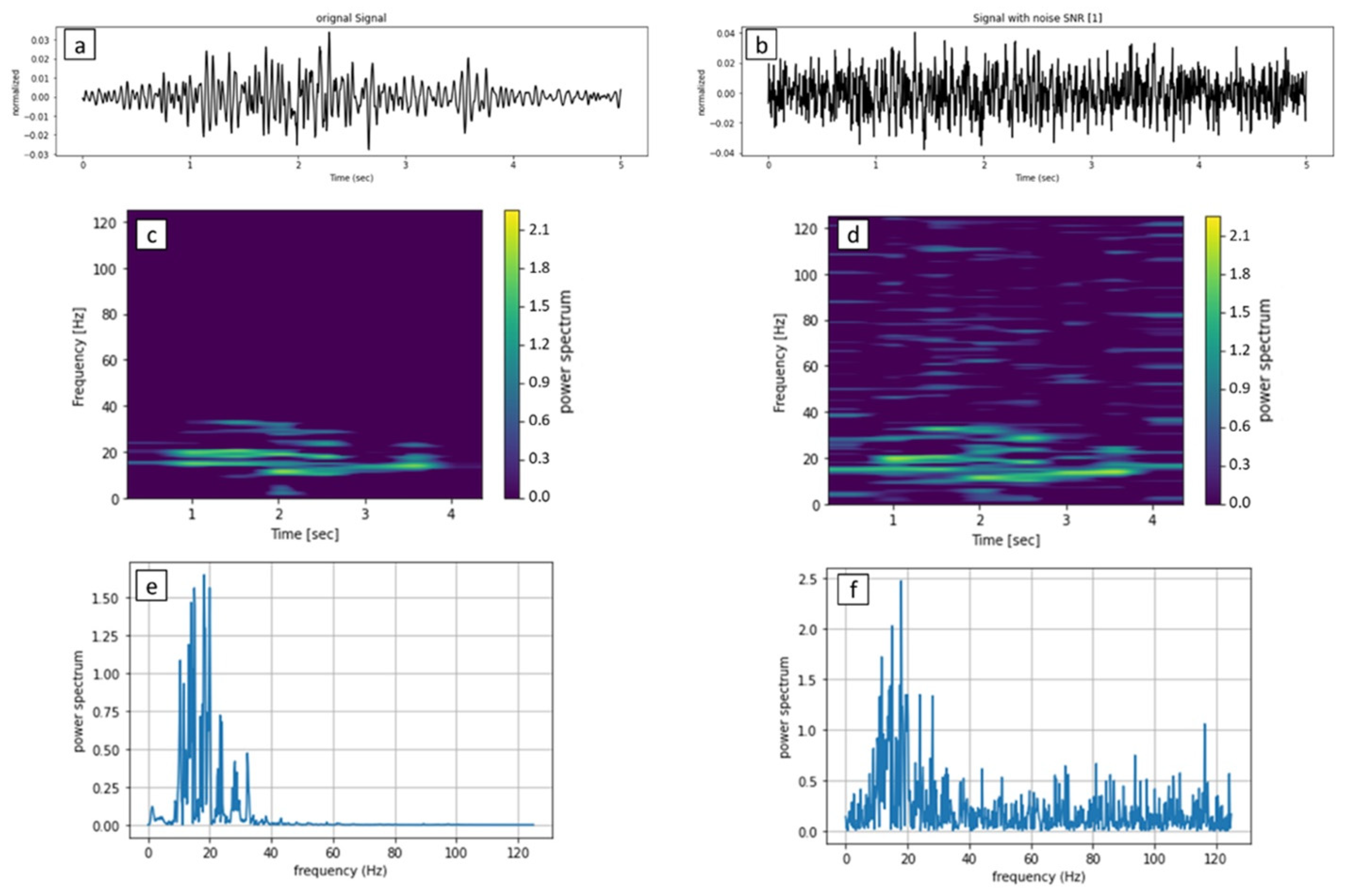
2.2. Training Data Augmentation

Extensive training data set is required in ML for precise prediction and to avoid overfitting [33]. For this reason, our initial dataset of 930 samples was inadequate, and therefore we created extra synthetic data from it for training. In order to alter the signal-to-noise ratio (SNR) of waveforms, random noise was applied, as shown in Figure 3. We varied the SNR [34] from 1 to 5, as determined by the following expression:
SNR = Psignal/Pnoise = (Asignal/Anoise)2,
where A is the root mean square amplitude and P is the average power. ~4650 artificial samples were employed in the enhanced dataset created and used for training.

2.3. Machine Learning Schemes

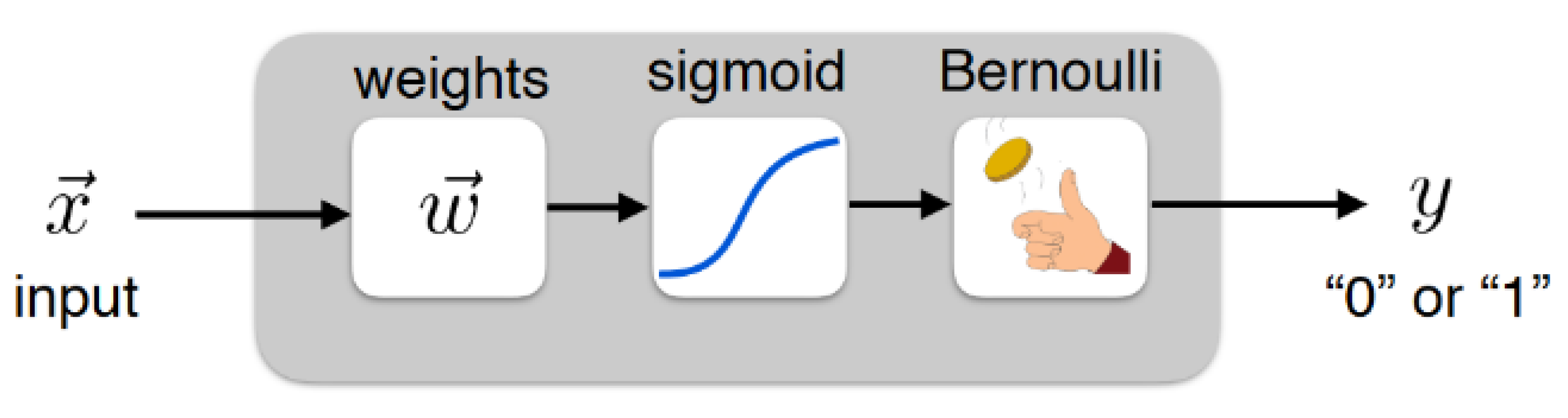
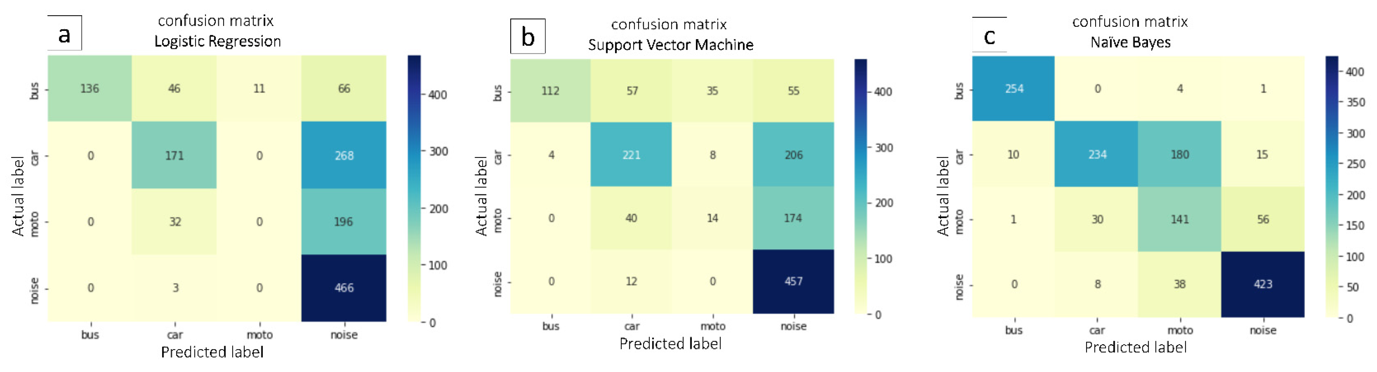
2.3.1. Logistic Regression (LR) for ML

The probability of a target variable is predicted using the supervised learning classification technique known as logistic regression. In LR, we take the output of the linear function and compress the value to the range of [0, 1] using the sigmoid function (logistic function). Any real-valued integer may be mapped to a value between 0 and 1 using the sigmoid function, which is an S-shaped curve but never precisely at those values [35]. For building our classifier model, we used generalized linear models with LR (Figure 4).
A logistic regression model makes mathematical predictions about P(Y = 1) as a function of X. Several category problems, including spam detection and diabetes prediction, may be solved using one of the most fundamental machine learning methods.

2.3.2. Support Vector Machine (SVM)

SVM algorithm was implemented in Matlab to train SVM classifiers for model-building and then use the optimal classifier for new data classification. We used SVM with a non-linear kernel, e.g., a radial basis function. The traditional C-SVM model was used as a classification model and can be described as follows:
1 2   w 2 + C i = 1 l ζ i   ,
y i [ w · x i + b ] 1 ζ i ,   ( ζ i 0 ) ,   i = 1 , 2 , 3   l   ,
where w is the average vector, C is the penalty factor, and ζi is the margin of error. xi is the input, yi is the class label, b is the bias to the separation hyperplane, and l is the number of samples of the input xi.
Additionally, the radial basis kernel function, which was applied to address the non-linear characteristics of the geophysical data, can be described as:
K ( x i , x j ) = e x p ( g x i x j 2 ) ,   g > 0   ,
where g is the kernel parameter that denotes the transformed data’s gamma distribution, and the kernel parameter g, and penalty factor C are adjusted to search for optimal separation hyperplane. We used ten-fold cross-validation for training classifiers to avoid overfitting. In contrast, the SVM approach involves adopting a non-linear kernel function to transform the input data into a higher-dimensional feature space, making it easier to separate the data. The iterative learning process in SVM identifies the optimal hyperplanes with the maximum margin between each class in a higher-dimensional feature space.

2.3.3. Naïve Bayes (NB)

NB is a probabilistic classifier that applies Bayes’ theorem with strong (naïve) independence assumptions between the features. The following was used to calculate a posterior probability of A happening given that B happened:
P ( A B ) = P ( A B ) / P ( B ) = P ( A ) × P ( B A ) / P ( B ) ,
where A and B are events or classes, P(A) and P(B) are the probabilities of A occurring and B occurring independently of each other. P(B) should be greater than zero, and P(BA) is the probability of B occurring, given that A is true. Bayes’ Rule was applied to our classification problem; we classified our data into the population that maximizes the posterior probability for the decision rule.

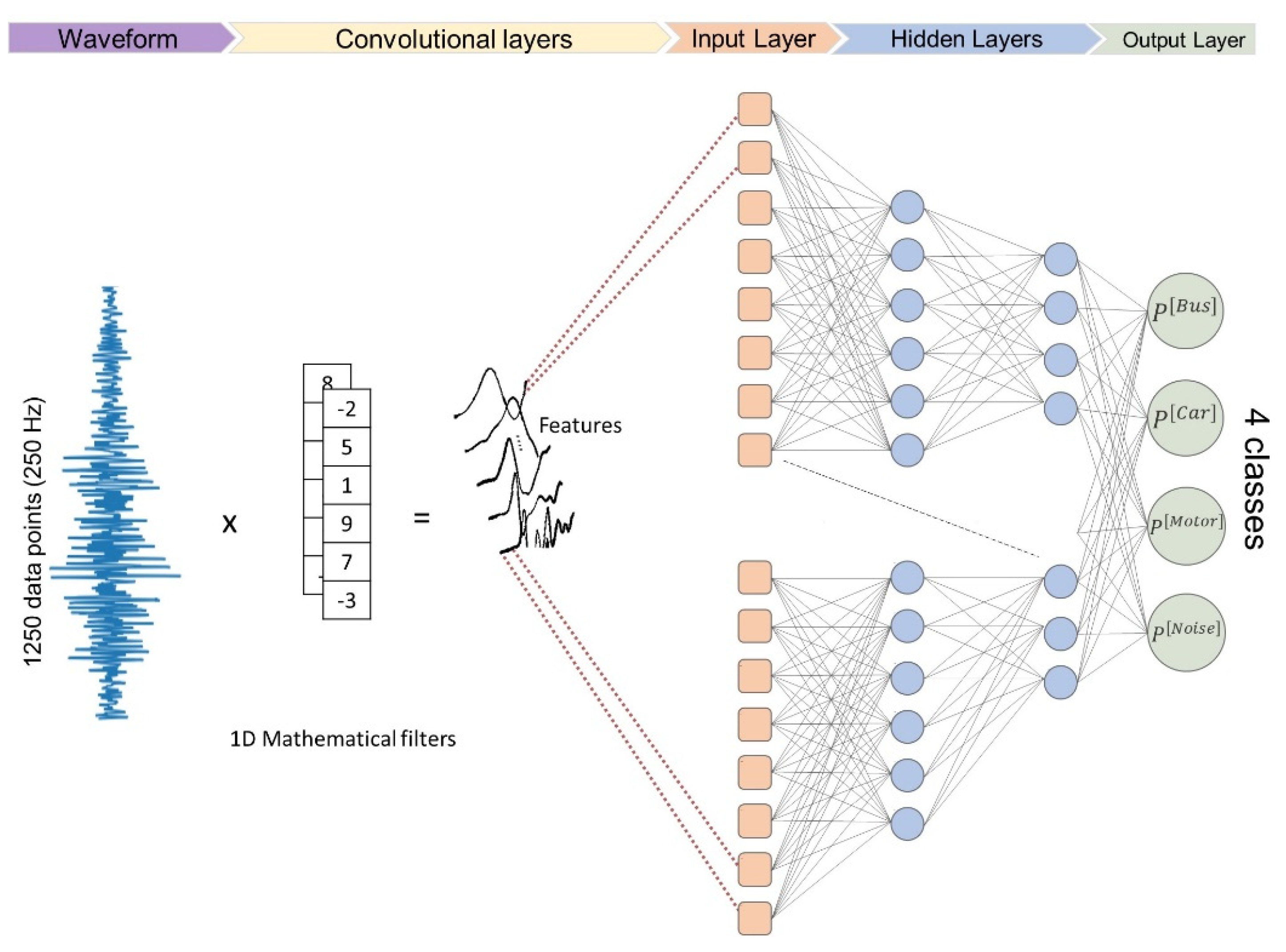
2.3.4. Convolutional Neural Networks (CNNs)

Neural Networks form the main backbone for deep learning. CNN is an enhanced neural network design. This AI technique was inspired by biological processes between neurons of the animal visual cortex [36]. In this study, we used CNNs to compare the performance of ML, and deep learning (DL) approaches. CNNs use filters before the neural networks called the convolutional layer. In our CNN, we used multiple convolutional layers with multi-channel filters in each layer and maximum pooling. The convolutional layer extracts the unique features and passes them to the neural networks. CNN breaks problems into smaller-scale tasks, making it an effective method for solving complex problems. Every neuron in each layer holds values depending on the previous input layer, and the weight connecting the neurons is given by:
Y = 1 n ( X * W ) + b   ,
where n represents the number of neurons in a hidden layer, X is the value that the neuron holds, W represents the weight that connects Y with X, and b is the bias for the equation.
We used published CNN architecture shown in Figure 5. The architecture contains five convolutional layers, each containing 50 1D mathematical filters. After the mathematical filter for downsampling, we used the MaxPool layer with dimensions (1 × 3). The CNN contains four hidden layers with redactional size, and the final layer is four output classes normalized with the softmax equation to 0 and 1 [32]. We used the pre-trained CNN model for comparison with the other three ML methods.

3. Results and Discussion

We calculated precision, recall, f1-score, and accuracy to evaluate the three proposed methods using the same training and test data set [37]. The formula for each evaluation technique is described as the following equation:
P r e c i s i o n = T r u e   P o s i t i v e T r u e   P o s t i v e + F a l s e   P o s t i v e   ,
R e c a l l = T r u e   P o s i t i v e T r u e   P o s i t i v e + F a l s e   N e g a t i v e     ,
f 1 - s c o r e = 2 × P r e c i s i o n × R e c a l l P r e c i s i o n + R e c a l l     ,
A c c u r a c y = T r u e   P o s i t i v e + T r u e   N e g a t i v e   a l l   p r e d i c t i o n s     ,
We randomly split the dataset into training and testing data sets in a 75–25 ratio. The testing data set includes (259 buses, 439 cars, 228 motorcycles, and 469 noise) data samples, including actual and synthetic data.
We used a confusion matrix heat map to visualize the performance of LR, SVM, and NB shown in Figure 6. Apart from the decision accuracy evaluation, we measured the computational time for the three methods and compared those results with the state-of-the-art CNN architecture.
The confusion matrix of LR detection is presented in Figure 6a. Table 1 shows the precision, recall, and f1-score for each class of LR calculated based on the result of Figure 6a. Based on Figure 6a, LR has failed to detect any motorcycle signals, while it has overpredicted the noise, especially for car and motorcycle classes.
LR has made 11 predictions for a motorcycle, but all were false positive predictions toward the bus class, as shown in Figure 6a. Table 1 shows that LR scores 99% precision for the noise class and 47% recall only for the same class. On the other hand, LR scores 100% recall and 53% precision for the bus class. These scores indicate that the LR classifier is unsuitable for the proposed task and will probably miss or incorrectly detect the right vehicle’s class. Figure 6b shows the decisions made by the SVM model. We can see a slight improvement compared to LR model predictions. Based on Figure 6b and Table 2, SVM has 14 true positive motorcycle predictions. However, the SVM’s scores are relatively too low to be a reliable method for the given task.
The third algorithm we tested in this study (NB) has significantly improved prediction scores. NB could successfully predict most motorcycle data samples, which LR and SVM failed to do. NB has also sourced 98% precision and 97% f1-score for the bus class, as shown in Table 3. NB scored a 47% f1-score for the motorcycle class, considered the highest among the three methods. NB has scored relatively high precision, recall, and f1-scores which might make it a potential competitor for the CNN algorithm in this task.
In addition to the previous evaluation parameters, we have calculated the accuracy using equation 10, measured the running time for all three methods, and compared it with the accuracy and running time for CNN, as shown in Table 4. We used a work frame consisting of Python code based on ObsPy, NumPy, and scikit-learn libraries for this task. We used a cloud computing platform containing dual Tesla K80 GPUs with 12 GB RAM to run all algorithms. While CNN still scores the highest accuracy along all proposed methods, NB has 750 times faster computation time. While CNN required 112 s to finalize the training and test, NB needed 0.15 s to do the same task using an identical data set.

4. Conclusions

We have tested three ML algorithms, Logistic Regression, Support Vector Machine, and Naïve Bayes, using the same data set to investigate which is suitable for traffic monitoring based on the ground motion generated by vehicles. We have observed four factors in training and testing to evaluate the efficiency of the methods and have compared them to the state-of-the-art CNN using 5580 data samples. After testing and observation, we find that both Logistic Regression and Support Vector Machine are not suitable for the mentioned task. Logistic Regression and Support Vector Machine scored low in all evaluations. LR and SVM failed to recognize any motorcycle seismic signals, and both of them have low precision for vehicles and high precision for noise, indicating that these methods frequently mispredicted vehicles as noise. SVM was computationally expensive relative to the other ML algorithm. Therefore, we do not recommend considering Logistic Regression nor Support Vector Machine for the given task.
On the other hand, Naïve Bayes has shown promising results. NB has average F-1 scores of 75%, up to 97% in some cases. NB did not have difficulty correctly predicting motorcycles and scored 62% precision. Although CNN is the superior method in accuracy and precision, Naïve Bayes has shown modest computational cost. NB was 750 times faster than CNN under the same conditions. We recommend developing and enhancing models for traffic monitoring using NB with frequency domain data. We will consider this factor in future research. Therefore, we recommend NB for vehicle classification application that has real-time processing. Otherwise, CNN can be adopted for offline applications based on the significant compromise on accuracy.
However, this approach faces some challenges as the current approach is limited to a single-vehicle pass; this problem may be overcome by installing two or more geophones within a known distance near the roadway. Another consideration that should be studied in the future is real-time monitoring. So far, all studies have used seismic data records but not real-time data. We will consider this purpose in future research. The proposed method can be further enhanced by forecasting various aspects of traffic flow, such as speed, direction, and whether a road user is driving safely. This approach may also be adapted and applied to other modes of transportation, including ships, bicycles, foot traffic, and airplanes.

Author Contributions

All authors contributed to this study. Conceptualization, A.B.A., H.S. and T.T.; data curation, A.B.A.; formal analysis, A.B.A.; funding acquisition, T.T.; investigation, H.S. and T.T.; methodology, A.B.A., T.T., H.S. and A.N.B.; resources, T.T. and H.S.; software, A.B.A. and A.N.B.; visualization, T.T. and H.S.; writing—original draft, A.B.A. and H.S.; writing—review and editing, H.S. All authors have read and agreed to the published version of the manuscript.

Funding

This work was supported by JSPS KAKENHI Grant Number JP20H01997 and JP21H05202. Furthermore, the approach for automatic signal classification was partially supported by Shikoku Electric Power Co., Inc.

Data Availability Statement

The seismic data sets are available by communicating with the authors.

Acknowledgments

Chanmaly CHHUN, Fernando LAWRENS, Rezkia DEWI, Fahrudin, and Tarek IMAM (Kyushu University, Japan) are acknowledged by ABA and TT for their assistance in gathering seismic data. HS and ANB thank UAEU for providing Matlab and the computing resources needed to execute the simulation.

Conflicts of Interest

The authors declare no conflict of interest.

References

  1. Lee, H.; Coifman, B. Using LIDAR to Validate the Performance of Vehicle Classification Stations. J. Intell. Transp. Syst. Technol. Plan. Oper. 2015, 19, 355–369. [Google Scholar] [CrossRef]
  2. U.S. Federal Highway Administration (Ed.) Traffic Monitoring Guide—Updated October 2016; Office of Highway Policy Information: Washington, DC, USA, 2016; pp. 56–59.
  3. Abiodun, O.I.; Jantan, A.; Omolara, A.E.; Dada, K.V.; Mohamed, N.A.; Arshad, H. State-of-the-art in artificial neural network applications: A survey. Heliyon 2018, 4, e00938. [Google Scholar] [CrossRef] [PubMed]
  4. Won, M. Intelligent Traffic Monitoring Systems for Vehicle Classification: A Survey. IEEE Access 2019, 8, 73340–73358. [Google Scholar] [CrossRef]
  5. Coifman, B.; Neelisetty, S. Improved Speed Estimation from Single-Loop Detectors with High Truck Flow. J. Intell. Transp. Syst. Technol. Plan. Oper. 2014, 18, 138–148. [Google Scholar] [CrossRef]
  6. Jeng, S.-T.; Chu, L. A high-definition traffic performance monitoring system with the Inductive Loop Detector signature technology. In Proceedings of the 2014 17th IEEE International Conference on Intelligent Transportation Systems, ITSC 2014, Qingdao, China, 14 November 2014; pp. 1820–1825. [Google Scholar] [CrossRef]
  7. Wu, L.; Coifman, B. Improved vehicle classification from dual-loop detectors in congested traffic. Transp. Res. Part C Emerg. Technol. 2014, 46, 222–234. [Google Scholar] [CrossRef]
  8. Wu, L.; Coifman, B. Vehicle Length Measurement and Length-Based Vehicle Classification in Congested Freeway Traffic. Transp. Res. Rec. 2014, 2443, 1–11. [Google Scholar] [CrossRef]
  9. Balid, W.; Refai, H.H. Real-Time Magnetic Length-Based Vehicle Classification: Case Study for Inductive Loops and Wireless Magnetometer Sensors in Oklahoma State. Transp. Res. Rec. 2018, 2672, 102–111. [Google Scholar] [CrossRef]
  10. Li, Y.; Tok, A.Y.C.; Ritchie, S. Individual Truck Speed Estimation from Advanced Single Inductive Loops. Transp. Res. Rec. 2019, 2673, 272–284. [Google Scholar] [CrossRef]
  11. Lamas-Seco, J.J.; Castro, P.M.; Dapena, A.; Vazquez-Araujo, F.J. Vehicle Classification Using the Discrete Fourier Transform with Traffic Inductive Sensors. Sensors 2015, 15, 27201–27214. [Google Scholar] [CrossRef] [Green Version]
  12. Dong, H.; Wang, X.; Zhang, C.; He, R.; Jia, L.; Qin, Y. Improved Robust Vehicle Detection and Identification Based on Single Magnetic Sensor. IEEE Access 2018, 6, 5247–5255. [Google Scholar] [CrossRef]
  13. Belenguer, F.M.; Martinez-Millana, A.; Salcedo, A.M.; Núñez, J.H.A. Vehicle Identification by Means of Radio-Frequency-Identification Cards and Magnetic Loops. IEEE Trans. Intell. Transp. Syst. 2019, 21, 5051–5059. [Google Scholar] [CrossRef]
  14. Li, F.; Lv, Z. Reliable vehicle type recognition based on information fusion in multiple sensor networks. Comput. Netw. 2017, 117, 76–84. [Google Scholar] [CrossRef]
  15. Odat, E.; Shamma, J.S.; Claudel, C. Vehicle Classification and Speed Estimation Using Combined Passive Infrared/Ultrasonic Sensors. IEEE Trans. Intell. Transp. Syst. 2018, 19, 1593–1606. [Google Scholar] [CrossRef]
  16. Carli, R.; Dotoli, M.; Epicoco, N.; Angelico, B.; Vinciullo, A. Automated Evaluation of Urban Traffic Congestion Using Bus as a Probe. In Proceedings of the 2015 IEEE International Conference on Automation Science and Engineering (CASE), Gothenburg, Sweden, 24–28 August 2015; pp. 967–972. [Google Scholar]
  17. Ahmed, S.H.; Bouk, S.H.; Yaqub, M.A.; Kim, D.; Song, H.; Lloret, J. CODIE: Controlled Data and Interest Evaluation in Vehicular Named Data Networks. IEEE Trans. Veh. Technol. 2016, 65, 3954–3963. [Google Scholar] [CrossRef]
  18. Carli, R.; Dotoli, M.; Epicoco, N. Monitoring traffic congestion in urban areas through probe vehicles: A case study analysis. Internet Technol. Lett. 2018, 1, e5. [Google Scholar] [CrossRef]
  19. Wang, S.; Zhang, X.; Cao, J.; He, L.; Stenneth, L.; Yu, P.S.; Li, Z.; Huang, Z. Computing Urban Traffic Congestions by Incorporating Sparse GPS Probe Data and Social Media Data. ACM Trans. Inf. Syst. 2017, 35, 1–30. [Google Scholar] [CrossRef]
  20. Litman, T. Developing Indicators for Comprehensive and Sustainable Transport Planning. Transp. Res. Rec. 2007, 2017, 10–15. [Google Scholar] [CrossRef]
  21. Martin, P.T.; Feng, Y.; Wang, X.; Assistants, R. Detector Technology Evaluation; Mountain-Plains Consortium: Fargo, ND, USA, 2003. [Google Scholar]
  22. William, P.E.; Hoffman, M.W. Classification of Military Ground Vehicles Using Time Domain Harmonics’ Amplitudes. IEEE Trans. Instrum. Meas. 2011, 60, 3720–3731. [Google Scholar] [CrossRef]
  23. Ketcham, S.; Moran, M.; Lacombe, J.; Greenfield, R.; Anderson, T. Seismic source model for moving vehicles. IEEE Trans. Geosci. Remote Sens. 2005, 43, 248–256. [Google Scholar] [CrossRef]
  24. Moran, M.L.; Greenfield, R.J. Estimation of the Acoustic-to-Seismic Coupling Ratio Using a Moving Vehicle Source. IEEE Trans. Geosci. Remote Sens. 2008, 46, 2038–2043. [Google Scholar] [CrossRef]
  25. Jin, G.; Ye, B.; Wu, Y.; Qu, F. Vehicle Classification Based on Seismic Signatures Using Convolutional Neural Network. IEEE Geosci. Remote Sens. Lett. 2019, 16, 628–632. [Google Scholar] [CrossRef]
  26. Zhao, T. Seismic facies classification using different deep convolutional neural networks. In Proceedings of the 2018 SEG International Exposition and Annual Meeting, SEG 2018, Houston, TX, USA, 14–19 October 2018; pp. 2046–2050. [Google Scholar] [CrossRef]
  27. Shimshoni, Y.; Intrator, N. Classification of seismic signals by integrating ensembles of neural networks. IEEE Trans. Signal Process. 1998, 46, 1194–1201. [Google Scholar] [CrossRef]
  28. Zhao, T.; Mukhopadhyay, P. A Fault Detection Workflow Using Deep Learning and Image Processing. In Proceedings of the 2018 SEG International Exposition and Annual Meeting, SEG 2018, Houston, TX, USA, 14–19 October 2018; pp. 1966–1970. [Google Scholar]
  29. Perol, T.; Gharbi, M.; Denolle, M. Convolutional neural network for earthquake detection and location. Sci. Adv. 2018, 4, e1700578. [Google Scholar] [CrossRef] [PubMed]
  30. Yuan, S.; Liu, J.; Wang, S.; Wang, T.; Shi, P. Seismic Waveform Classification and First-Break Picking Using Convolution Neural Networks. IEEE Geosci. Remote Sens. Lett. 2018, 15, 272–276. [Google Scholar] [CrossRef]
  31. Evans, N. Automated Vehicle Detection and Classification Using Acoustic and Seismic Signals. Ph.D. Thesis, University of York, York, UK, 2010. [Google Scholar]
  32. Ahmad, A.; Tsuji, T. Traffic Monitoring System Based on Deep Learning and Seismometer Data. Appl. Sci. 2021, 11, 4590. [Google Scholar] [CrossRef]
  33. Waldeland, A.U.; Jensen, A.C.; Gelius, L.-J.; Solberg, A.H.S. Convolutional neural networks for automated seismic interpretation. Lead. Edge 2018, 37, 529–537. [Google Scholar] [CrossRef]
  34. Tyagi, V.; Kalyanaraman, S.; Krishnapuram, R. Vehicular Traffic Density State Estimation Based on Cumulative Road Acoustics. IEEE Trans. Intell. Transp. Syst. 2012, 13, 1156–1166. [Google Scholar] [CrossRef]
  35. Rymarczyk, T.; Kozłowski, E.; Kłosowski, G.; Niderla, K. Logistic Regression for Machine Learning in Process Tomography. Sensors 2019, 19, 3400. [Google Scholar] [CrossRef] [Green Version]
  36. Grossberg, S.; Rudd, M.E. A neural architecture for visual motion perception: Group and element apparent motion. Neural Netw. 1989, 2, 421–450. [Google Scholar] [CrossRef]
  37. Saibi, H.; Belkacem, A.N.; Amrouche, M. Cavity auto-detection using machine learning algorithms: Logistic regression, support vector machine, and naïve Bayes. In Proceedings of the Fifth International Conference on Engineering Geophysics, Al Ain, United Arab Emirates, 21–24 October 2019; pp. 260–263. [Google Scholar] [CrossRef]
Figure 1. A schematic illustration for the survey performed at Kyushu University to collect seismic data using three geophones (sensors) at a 15 m spacing and a 0.5 m distance from the road.
Computers 11 00148 g001
Figure 2. Example of signal plots for (a) a large vehicle (bus), (b) a medium-sized vehicle (light car), (c) a small vehicle (motorcycle), and (d) other noise (pedestrian). A yellow circle in each image indicates the seismic sensor (i.e., geophone).
Computers 11 00148 g002
Figure 3. (a) Seismic bus signal before adding noise. (b) Seismic signal after adding noise with SNR = 1. Panels (c,d) show the original and noisy signal spectrograms, respectively. Panels (e,f) show the power spectra calculated in the original and noisy signals, respectively.
Computers 11 00148 g003
Figure 4. Classification using generalized linear models with LR.
Computers 11 00148 g004
Figure 5. The CNN architecture was used in this study. The architecture contains five convolutional layers, a flatten (input layer), four dense layers, and four output classes.
Computers 11 00148 g005
Figure 6. A confusion matrix for prediction decisions for (a) LR model, (b) SVM model, and (c) NB model. The vertical axis shows the actual class, and the horizontal axis shows the predicted class by each model.
Computers 11 00148 g006
Table 1. The evaluation parameters for LR model prediction for 1395 data samples, including precision, recall, and f1-score calculated per class, averaged, and weighted average on the number of samples for each class.
PrecisionRecallF1-ScoreNumber of Predictions
Bus/Truck0.531.000.69136
Passenger car0.390.680.49252
Motorcycle0.000.000.0011
Noise0.990.470.64966
Average0.480.540.451395
Weighted average0.830.550.611395
Table 2. The evaluation parameters for SVM model prediction for 1395 data samples, including precision, recall, and f1-score calculated per class, averaged, and weighted average on the number of samples for each class.
PrecisionRecallF1-ScoreNumber of Predictions
Bus/Truck0.430.970.60116
Passenger car0.500.670.57330
Motorcycle0.060.250.1057
Noise0.970.510.67892
Average0.490.600.491395
Weighted average0.780.580.621395
Table 3. The evaluation parameters for NB model prediction for 1395 data samples, including precision, recall, and f1-score calculated per class, averaged, and weighted average on the number of samples for each class.
PrecisionRecallF1-ScoreNumber of Predictions
Bus/Truck0.980.960.97265
Passenger car0.530.860.66272
Motorcycle 0.620.390.48363
Noise0.900.850.88495
Average0.760.770.751395
Weighted average0.770.750.751395
Table 4. Accuracy and running time of LR, SVM, NB, and CNN. The running time includes the training and testing on data set with a size of 5580 samples.
LRSVMNBCNN
Accuracy55%58%75%94%
Running time (Seconds)1.66412.490.150112.3 *
* CNN has trained for 100 iterations.
Publisher’s Note: MDPI stays neutral with regard to jurisdictional claims in published maps and institutional affiliations.

