
In Silico Investigations of Multi-Drug Adaptive Therapy Protocols

 ,
,  ,
,  and
and 
Abstract
Simple Summary
Abstract
1. Introduction
2. Materials and Methods
2.1. Purpose
2.2. Entities, State Variables, and Scales
2.3. Process Overview and Scheduling
2.4. Design Concepts
2.4.1. Basic Principles
2.4.2. Emergence
2.4.3. Adaptation
2.4.4. Objectives
2.4.5. Learning
2.4.6. Prediction
2.4.7. Sensing
2.4.8. Interaction
2.4.9. Stochasticity
2.4.10. Collectives
2.4.11. Observation
2.5. Initialization
2.6. Input Data
2.7. Submodels
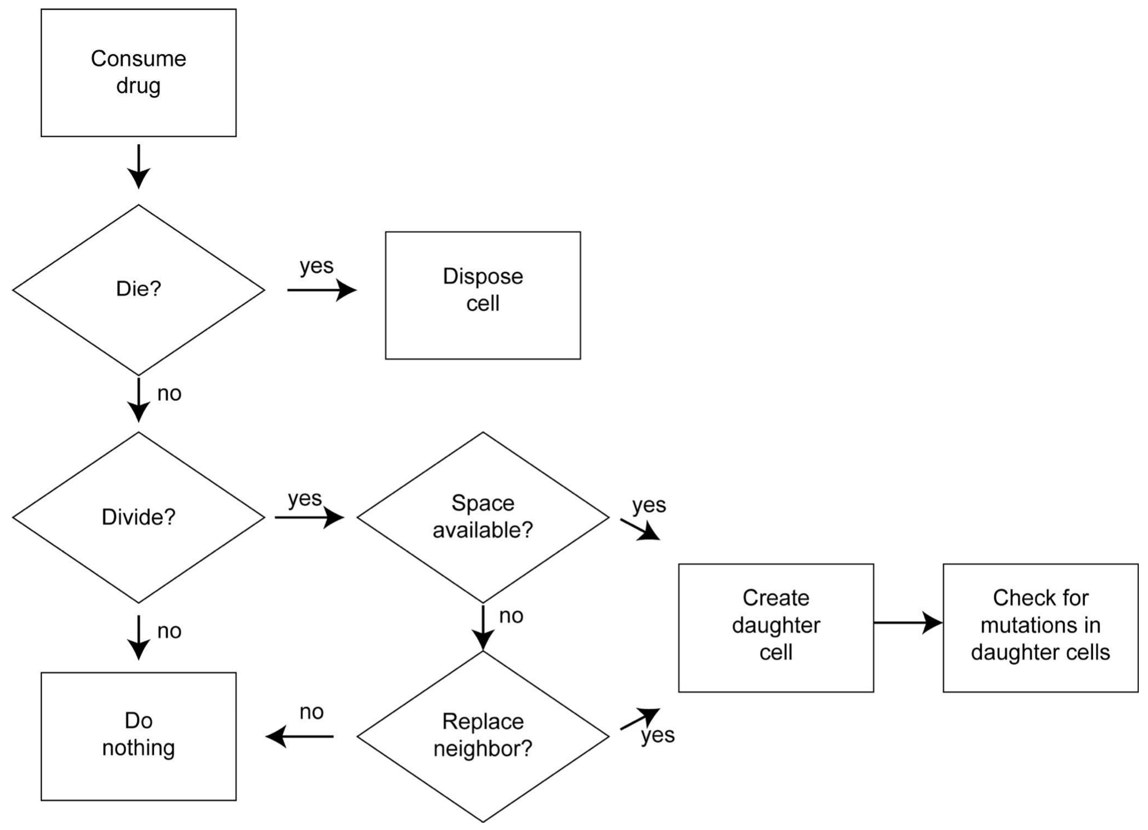
2.7.1. Cell Death
2.7.2. Cell Division
2.7.3. Competition for Space
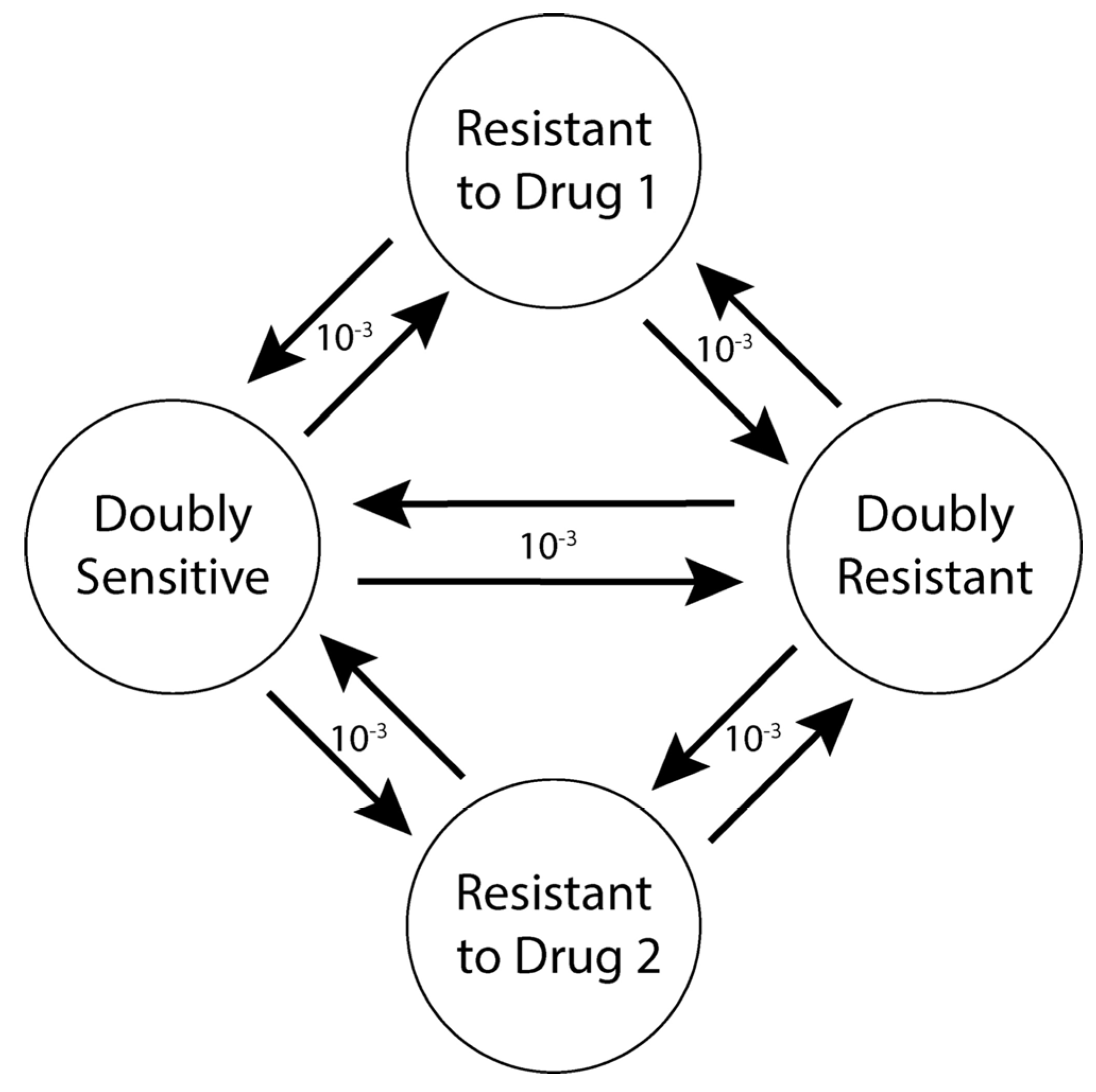
2.7.4. Mutation
2.7.5. Drug Dynamics (Diffusion and Metabolism)
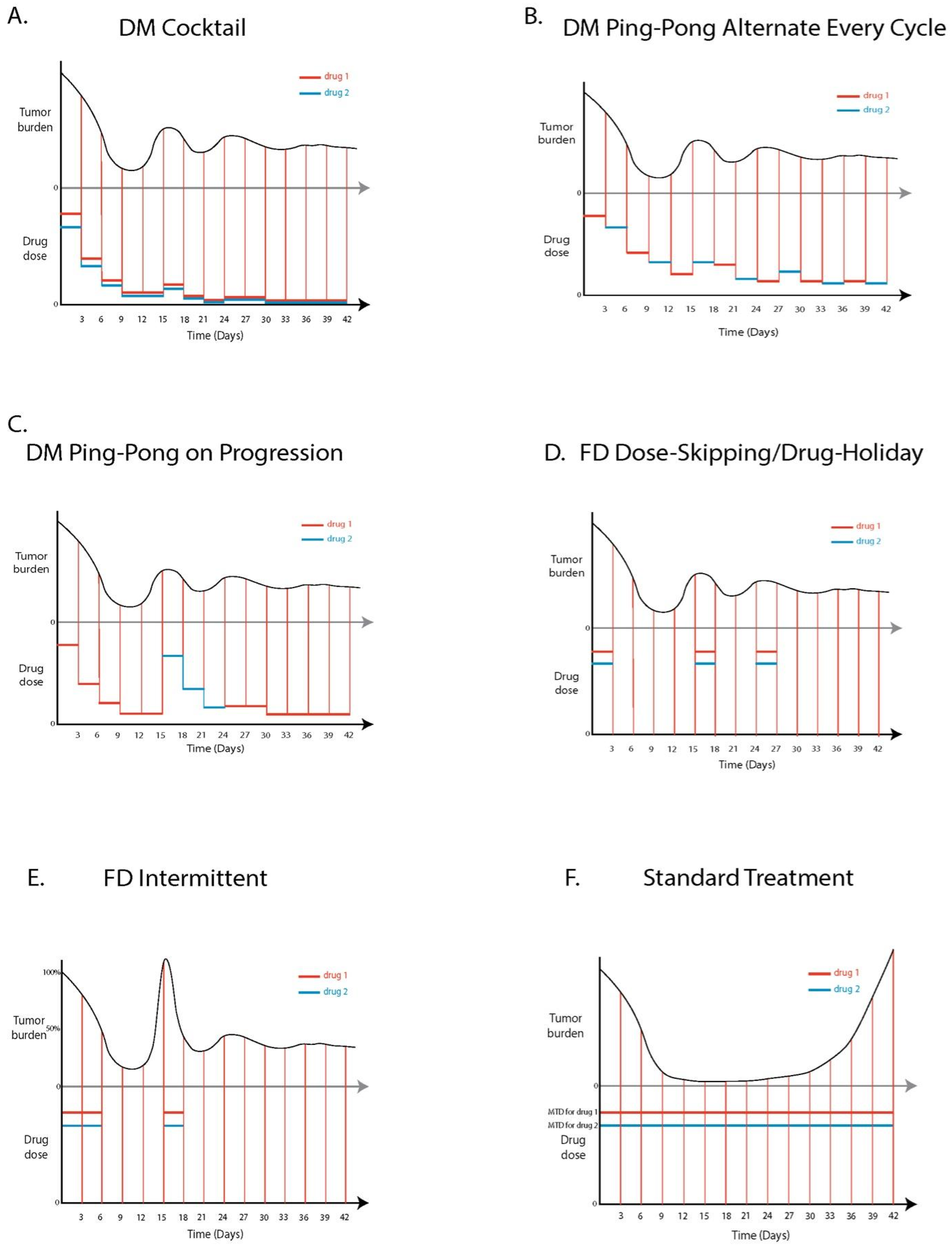
2.7.6. Drug Protocols
Standard Treatment (ST)
DM Cocktail Tandem
DM Ping-Pong Alternate Every Cycle
DM Ping-Pong on Progression
FD Dose-Skipping/Drug Holiday
FD Intermittent
3. Results
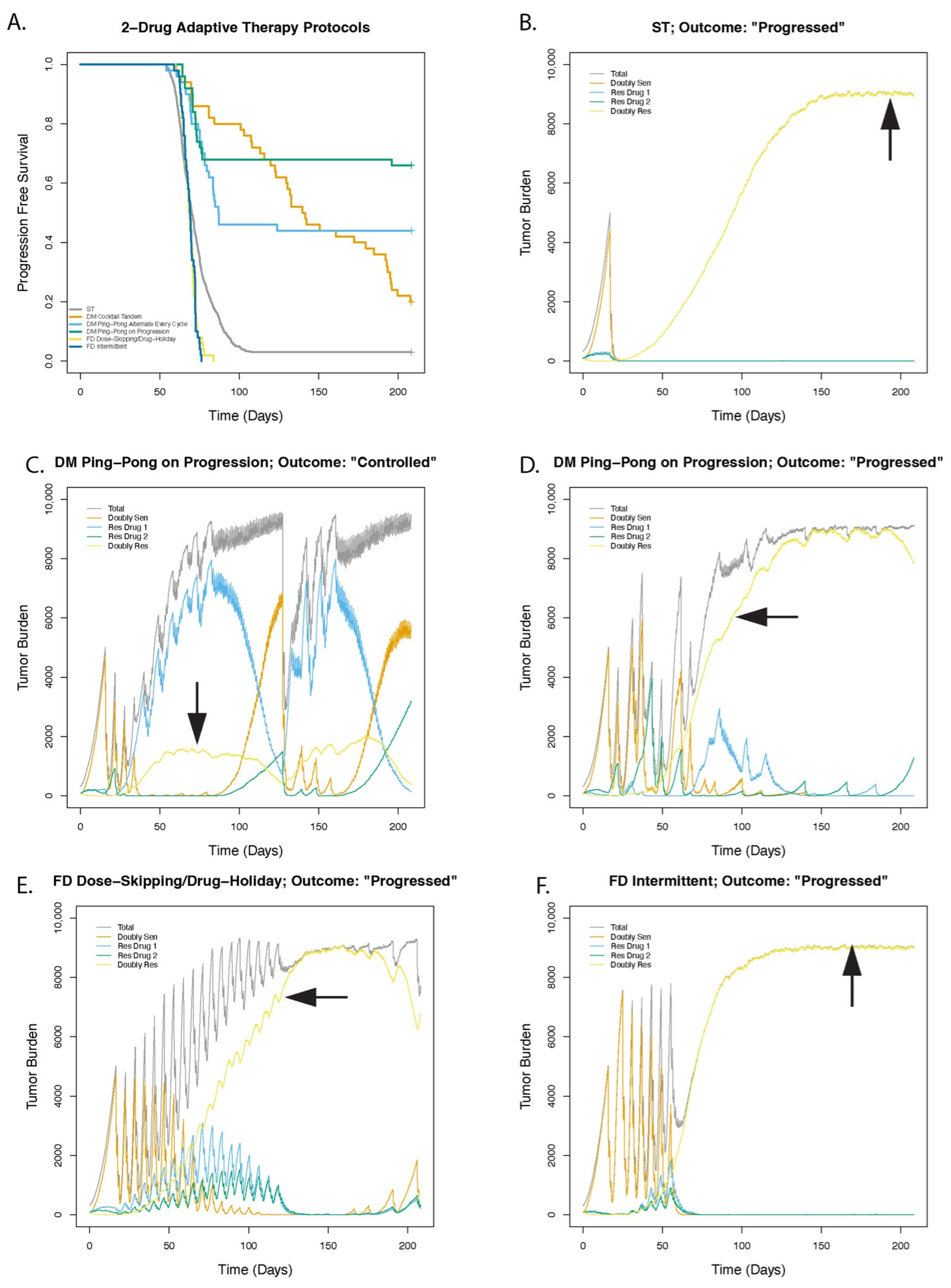
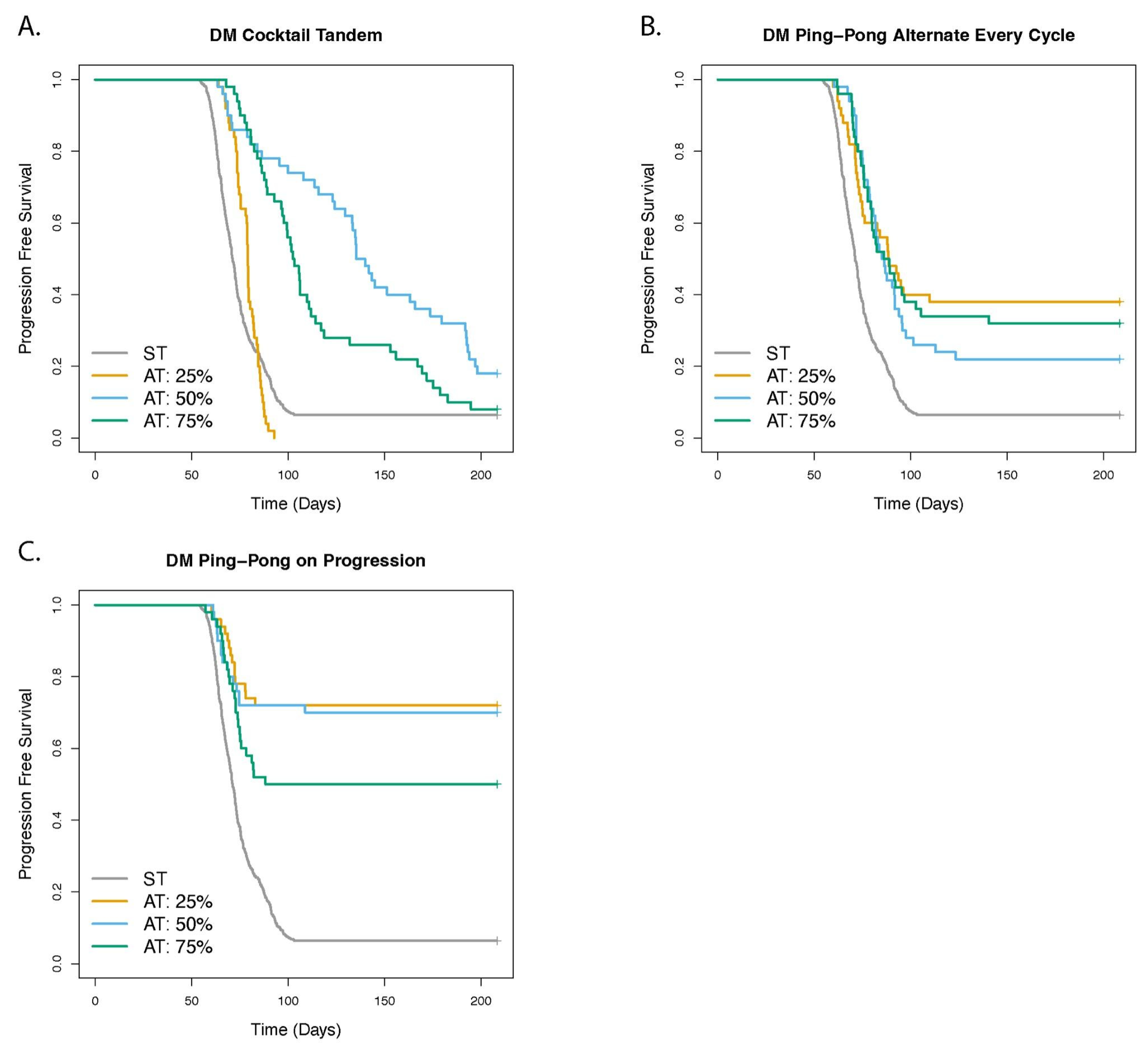
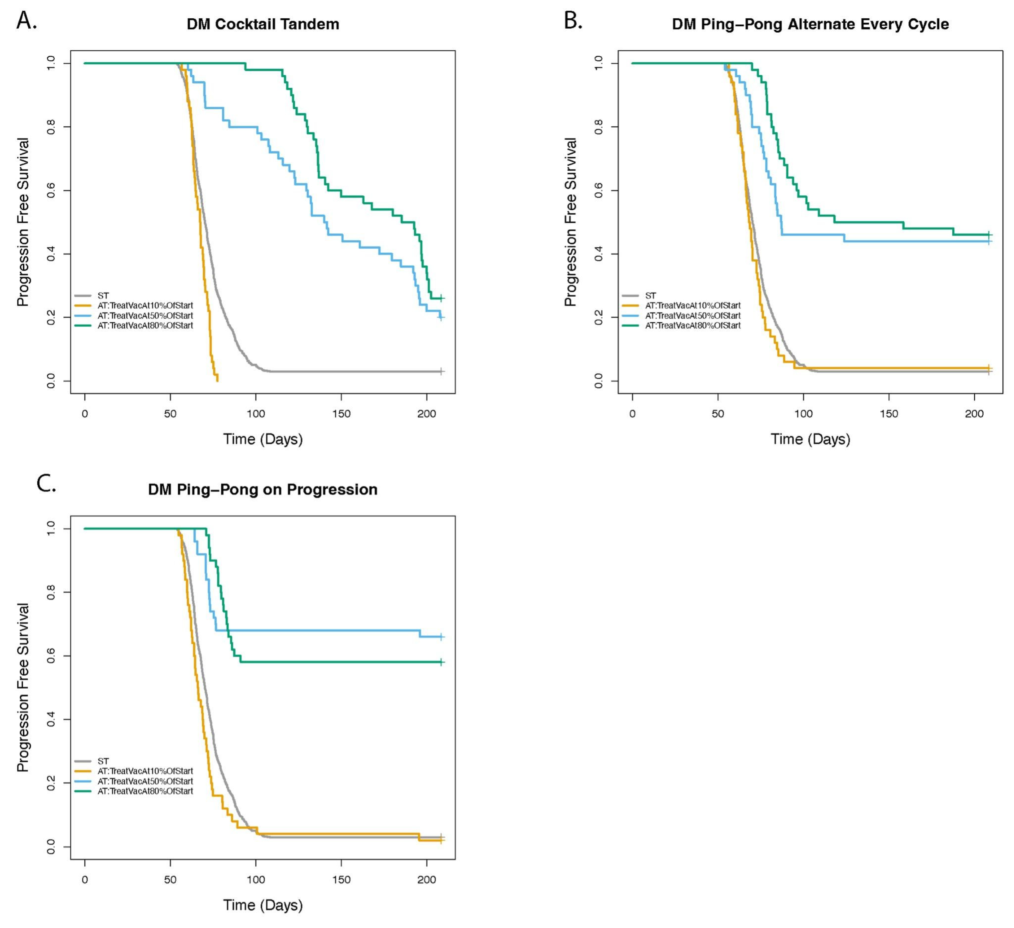
3.1. Dose Modulation Adaptive Therapy Protocols with Two Drugs Leads to Increased Time to Progression (TTP) Relative to Standard Treatment (ST) at Maximum Tolerated Dose
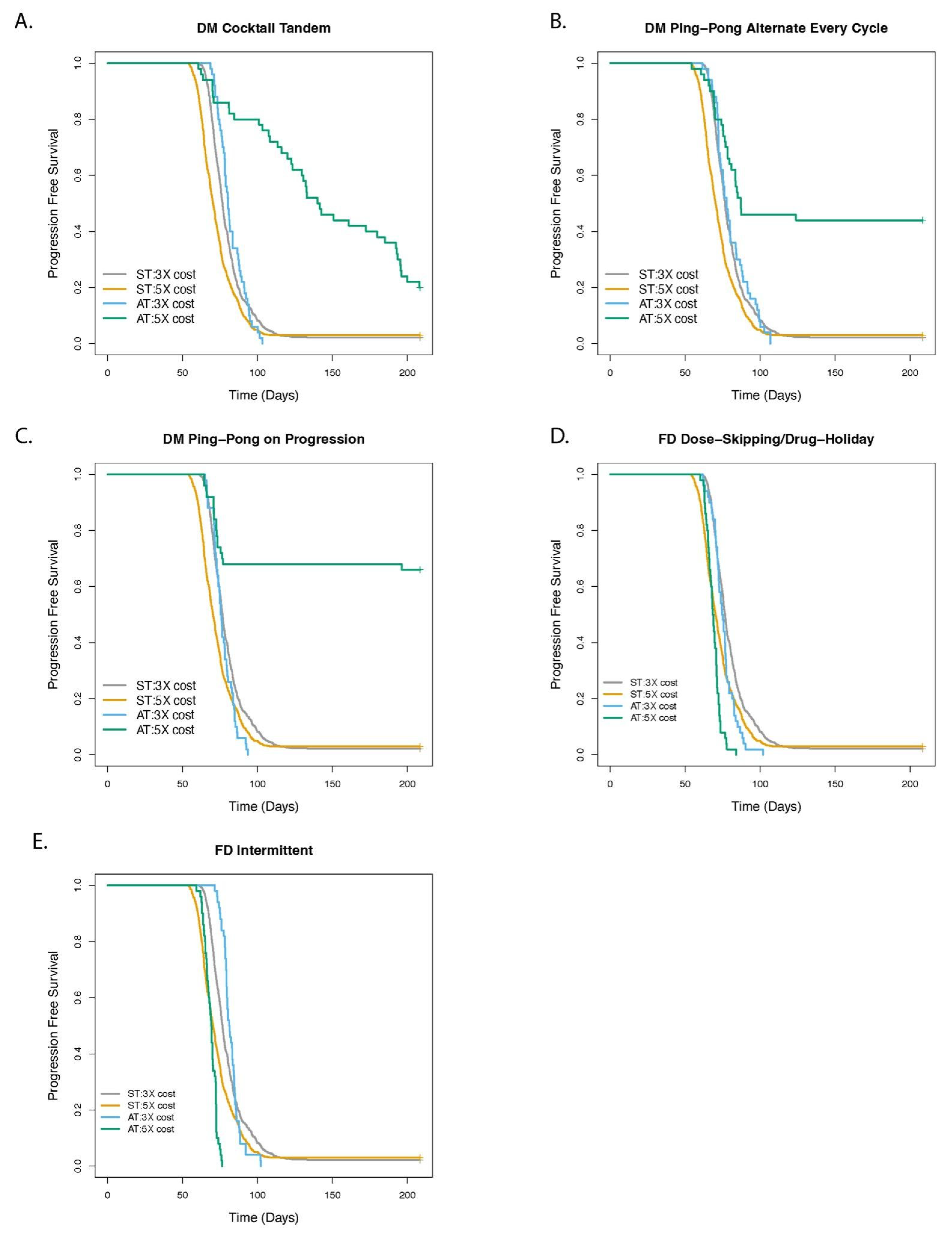
3.2. Greater Fitness Costs for Resistant Cells Increases the TTP for Adaptive Therapy
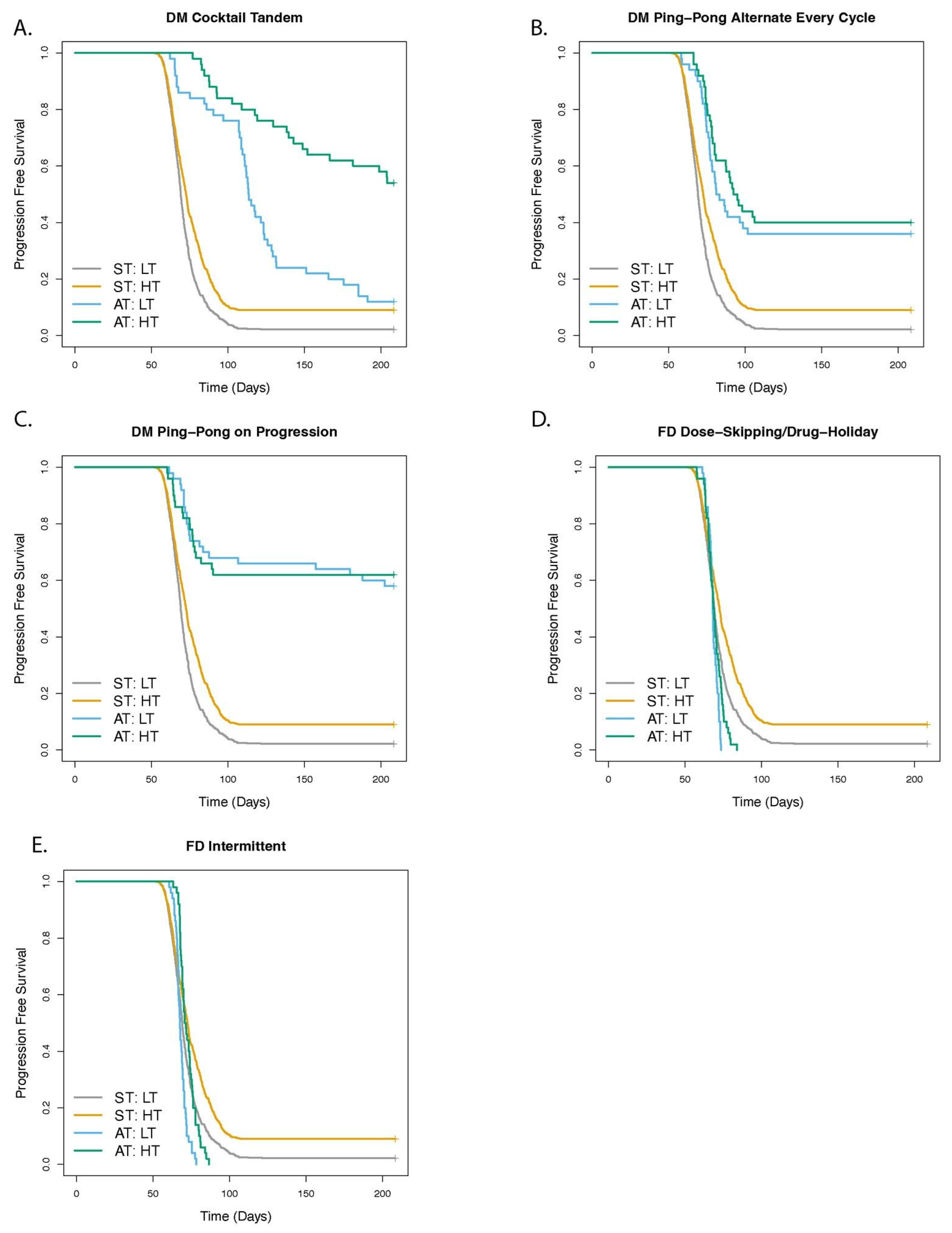
3.3. Higher Levels of Cell Turnover Increases the Efficacy of Adaptive Therapy
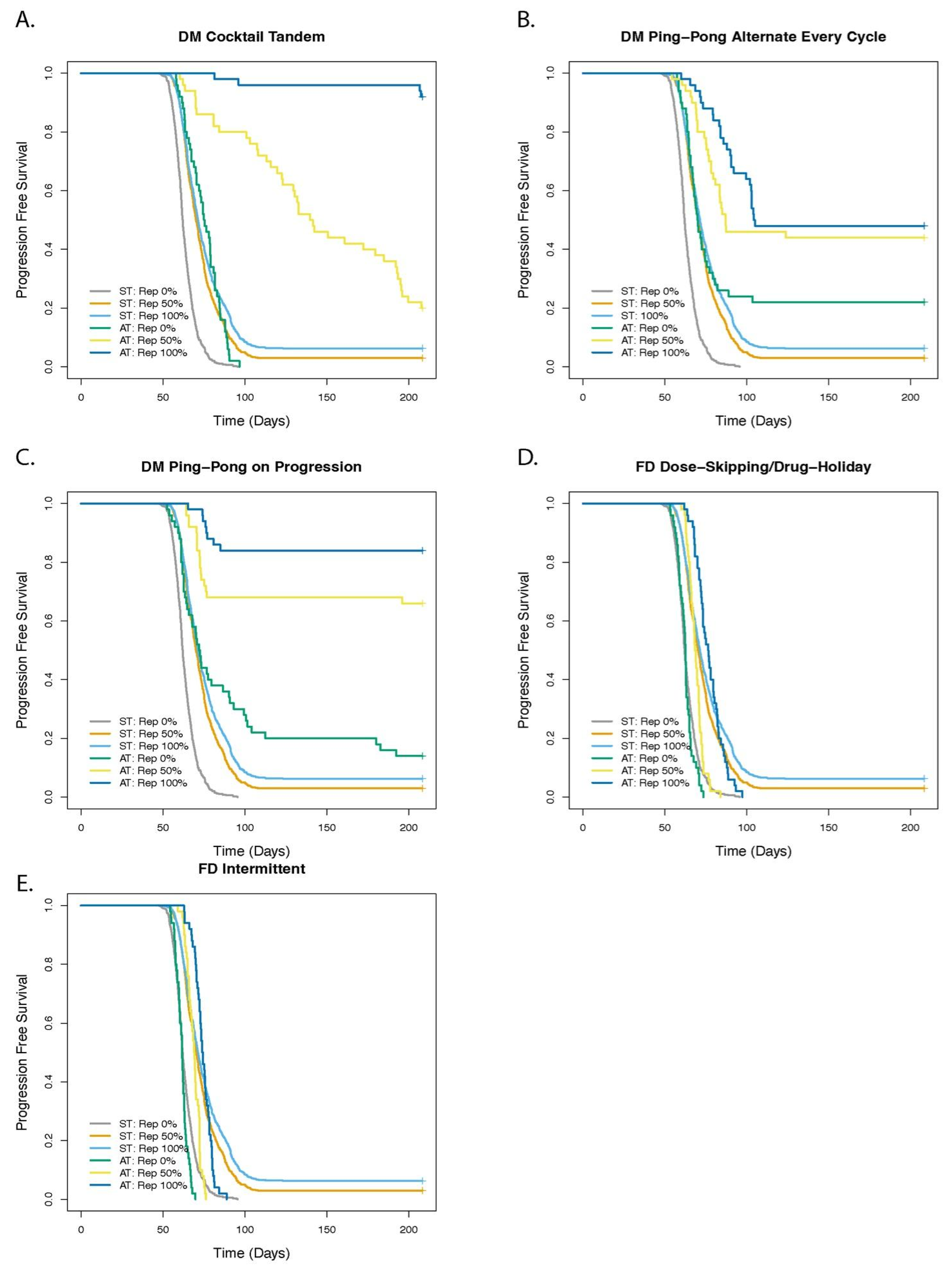
3.4. Cell Replacement Increases the TTP with Adaptive Therapy
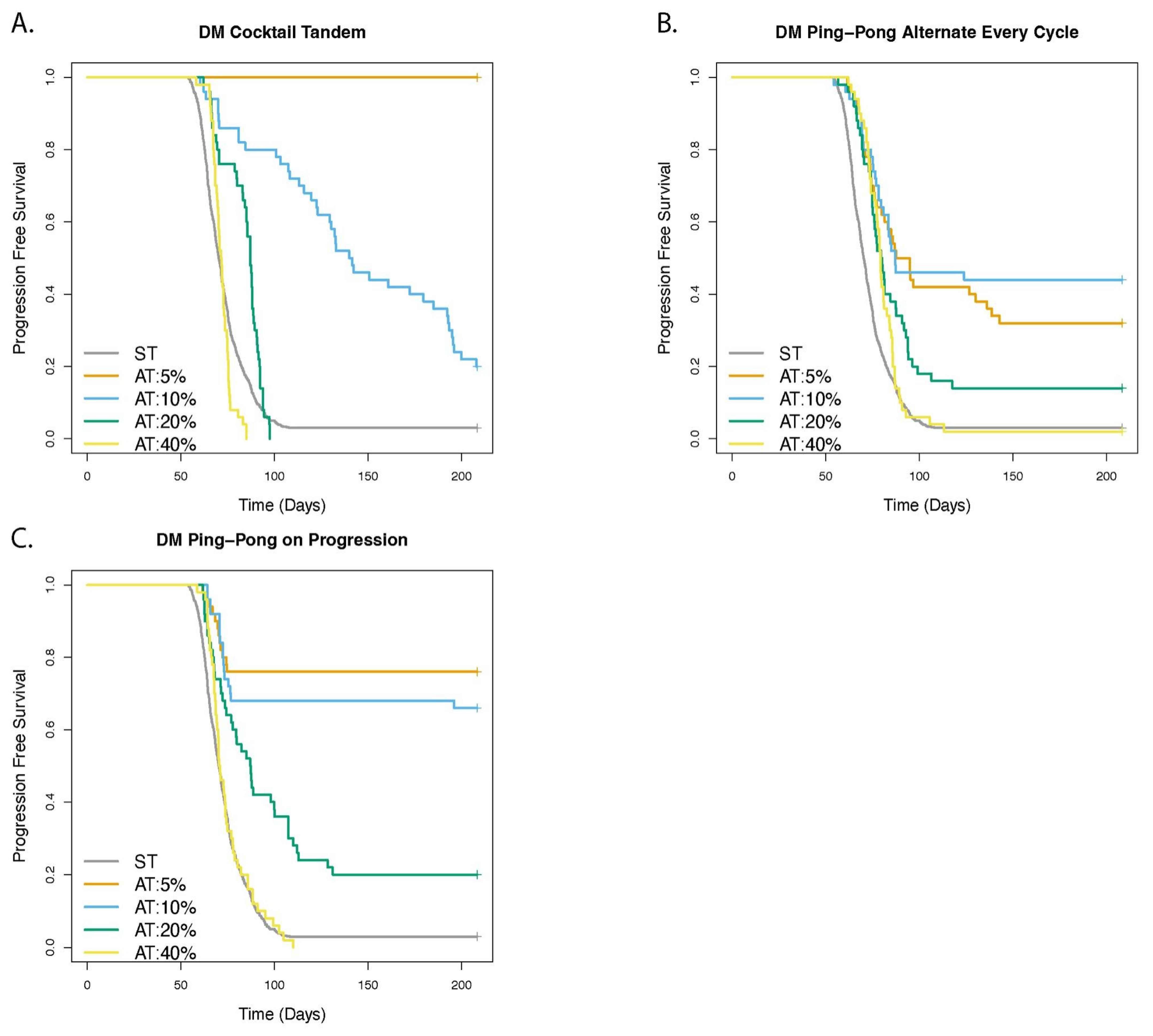
3.5. Adaptive Therapy Works Better If Smaller Changes in the Tumor Burden Trigger a Change in Dose
3.6. For Dose Modulation Regimens, the Amount by Which the Drug Dose Is Changed (Delta Dose) Has Little Effect on the Success of Adaptive Therapy
3.7. Dose Modulation Adaptive Therapy Works Best When Frequent Treatment Vacations Are Allowed
4. Discussion
5. Conclusions
Supplementary Materials
Author Contributions
Funding
Institutional Review Board Statement
Informed Consent Statement
Data Availability Statement
Acknowledgments
Conflicts of Interest
References
- Gatenby, R.A. A Change of Strategy in the War on Cancer. Nature 2009, 459, 508–509. [Google Scholar] [CrossRef] [PubMed]
- Chabner, B.A.; Roberts, T.G. Chemotherapy and the War on Cancer. Nat. Rev. Cancer 2005, 5, 65–72. [Google Scholar] [CrossRef] [PubMed]
- Williams, M.J.; Werner, B.; Barnes, C.P.; Graham, T.A.; Sottoriva, A. Identification of Neutral Tumor Evolution across Cancer Types. Nat. Genet. 2016, 48, 238–244. [Google Scholar] [CrossRef] [PubMed]
- Ross, E.M.; Markowetz, F. OncoNEM: Inferring Tumor Evolution from Single-Cell Sequencing Data. Genome Biol. 2016, 17, 69. [Google Scholar] [CrossRef] [PubMed]
- Ricketts, C.J.; Marston Linehan, W. Intratumoral Heterogeneity in Kidney Cancer. Nat. Genet. 2014, 46, 214–215. [Google Scholar] [CrossRef] [PubMed]
- Morris, L.G.T.; Riaz, N.; Desrichard, A.; Şenbabaoğlu, Y.; Ari Hakimi, A.; Makarov, V.; Reis-Filho, J.S.; Chan, T.A. Pan-Cancer Analysis of Intratumor Heterogeneity as a Prognostic Determinant of Survival. Oncotarget 2016, 7, 10051–10063. [Google Scholar] [CrossRef]
- Griffiths, J.I.; Chen, J.; Cosgrove, P.A.; O’Dea, A.; Sharma, P.; Ma, C.; Trivedi, M.; Kalinsky, K.; Wisinski, K.B.; O’Regan, R.; et al. Serial Single-Cell Genomics Reveals Convergent Subclonal Evolution of Resistance as Early-Stage Breast Cancer Patients Progress on Endocrine plus CDK4/6 Therapy. Nat. Cancer 2021, 2, 658–671. [Google Scholar] [CrossRef]
- Raatz, M.; Shah, S.; Chitadze, G.; Brüggemann, M.; Traulsen, A. The Impact of Phenotypic Heterogeneity of Tumour Cells on Treatment and Relapse Dynamics. PLoS Comput. Biol. 2021, 17, e1008702. [Google Scholar] [CrossRef]
- Kaznatcheev, A.; Peacock, J.; Basanta, D.; Marusyk, A.; Scott, J.G. Fibroblasts and Alectinib Switch the Evolutionary Games Played by Non-Small Cell Lung Cancer. Nat. Ecol. Evol. 2019, 3, 450–456. [Google Scholar] [CrossRef]
- Marusyk, A.; Almendro, V.; Polyak, K. Intra-Tumour Heterogeneity: A Looking Glass for Cancer? Nat. Rev. Cancer 2012, 12, 323–334. [Google Scholar] [CrossRef]
- Worsley, C.M.; Mayne, E.S.; Veale, R.B. Clone Wars: The Evolution of Therapeutic Resistance in Cancer. Evol. Med. Public Health 2016, 2016, 180–181. [Google Scholar] [CrossRef] [PubMed][Green Version]
- Ramos, P.; Bentires-Alj, M. Mechanism-Based Cancer Therapy: Resistance to Therapy, Therapy for Resistance. Oncogene 2015, 34, 3617–3626. [Google Scholar] [CrossRef]
- Barrett, M.T.; Lenkiewicz, E.; Evers, L.; Holley, T.; Ruiz, C.; Bubendorf, L.; Sekulic, A.; Ramanathan, R.K.; Von Hoff, D.D. Clonal Evolution and Therapeutic Resistance in Solid Tumors. Front. Pharmacol. 2013, 4, 2. [Google Scholar] [CrossRef] [PubMed]
- Enriquez-Navas, P.M.; Wojtkowiak, J.W.; Gatenby, R.A. Application of Evolutionary Principles to Cancer Therapy. Cancer Res. 2015, 75, 4675–4680. [Google Scholar] [CrossRef] [PubMed]
- Adkins, S.; Shabbir, A. Biology, Ecology and Management of the Invasive Parthenium Weed (Parthenium Hysterophorus L.). Pest Manag. Sci. 2014, 70, 1023–1029. [Google Scholar] [CrossRef] [PubMed]
- Alto, B.W.; Lampman, R.L.; Kesavaraju, B.; Muturi, E.J. Pesticide-Induced Release From Competition Among Competing Aedes Aegypti and Aedes Albopictus (Diptera: Culicidae). J. Med. Entomol. 2013, 50, 1240–1249. [Google Scholar] [CrossRef] [PubMed]
- Gallaher, J.A.; Enriquez-Navas, P.M.; Luddy, K.A.; Gatenby, R.A.; Anderson, A.R.A. Spatial Heterogeneity and Evolutionary Dynamics Modulate Time to Recurrence in Continuous and Adaptive Cancer Therapies. Cancer Res. 2018, 78, 2127–2139. [Google Scholar] [CrossRef]
- Gatenby, R.A.; Brown, J.; Vincent, T. Lessons from Applied Ecology: Cancer Control Using an Evolutionary Double Bind. Cancer Res. 2009, 69, 7499–7502. [Google Scholar] [CrossRef]
- Gatenby, R.A.; Silva, A.S.; Gillies, R.J.; Roy Frieden, B. Adaptive Therapy. Cancer Res. 2009, 69, 4894–4903. [Google Scholar] [CrossRef]
- Enriquez-Navas, P.M.; Kam, Y.; Das, T.; Hassan, S.; Silva, A.; Foroutan, P.; Ruiz, E.; Martinez, G.; Minton, S.; Gillies, R.J.; et al. Exploiting Evolutionary Principles to Prolong Tumor Control in Preclinical Models of Breast Cancer. Sci. Transl. Med. 2016, 8, 327ra24. [Google Scholar] [CrossRef]
- Zhang, J.; Cunningham, J.J.; Brown, J.S.; Gatenby, R.A. Integrating Evolutionary Dynamics into Treatment of Metastatic Castrate-Resistant Prostate Cancer. Nat. Commun. 2017, 8, 1816. [Google Scholar] [CrossRef] [PubMed]
- West, J.; You, L.; Zhang, J.; Gatenby, R.A.; Brown, J.S.; Newton, P.K.; Anderson, A.R.A. Towards Multidrug Adaptive Therapy. Cancer Res. 2020, 80, 1578–1589. [Google Scholar] [CrossRef] [PubMed]
- West, J.B.; Dinh, M.N.; Brown, J.S.; Zhang, J.; Anderson, A.R.; Gatenby, R.A. Multidrug Cancer Therapy in Metastatic Castrate-Resistant Prostate Cancer: An Evolution-Based Strategy. Clin. Cancer Res. 2019, 25, 4413–4421. [Google Scholar] [CrossRef] [PubMed]
- Ibrahim-Hashim, A.; Robertson-Tessi, M.; Enriquez-Navas, P.M.; Damaghi, M.; Balagurunathan, Y.; Wojtkowiak, J.W.; Russell, S.; Yoonseok, K.; Lloyd, M.C.; Bui, M.M.; et al. Defining Cancer Subpopulations by Adaptive Strategies Rather Than Molecular Properties Provides Novel Insights into Intratumoral Evolution. Cancer Res. 2017, 77, 2242–2254. [Google Scholar] [CrossRef]
- Bacevic, K.; Noble, R.; Soffar, A.; Wael Ammar, O.; Boszonyik, B.; Prieto, S.; Vincent, C.; Hochberg, M.E.; Krasinska, L.; Fisher, D. Spatial Competition Constrains Resistance to Targeted Cancer Therapy. Nat. Commun. 2017, 8, 1995. [Google Scholar] [CrossRef]
- Buhler, C.K.; Terry, R.S.; Link, K.G.; Adler, F.R. Do Mechanisms Matter? Comparing Cancer Treatment Strategies across Mathematical Models and Outcome Objectives. Math. Biosci. Eng. 2021, 18, 6305–6327. [Google Scholar] [CrossRef]
- Araujo, A.; Cook, L.M.; Frieling, J.S.; Tan, W.; Copland, J.A., 2nd; Kohli, M.; Gupta, S.; Dhillon, J.; Pow-Sang, J.; Lynch, C.C.; et al. Quantification and Optimization of Standard-of-Care Therapy to Delay the Emergence of Resistant Bone Metastatic Prostate Cancer. Cancers 2021, 13, 677. [Google Scholar] [CrossRef]
- Brady-Nicholls, R.; Nagy, J.D.; Gerke, T.A.; Zhang, T.; Wang, A.Z.; Zhang, J.; Gatenby, R.A.; Enderling, H. Prostate-Specific Antigen Dynamics Predict Individual Responses to Intermittent Androgen Deprivation. Nat. Commun. 2020, 11, 1750. [Google Scholar] [CrossRef]
- Cunningham, J.; Thuijsman, F.; Peeters, R.; Viossat, Y.; Brown, J.; Gatenby, R.; Staňková, K. Optimal Control to Reach Eco-Evolutionary Stability in Metastatic Castrate-Resistant Prostate Cancer. PLoS ONE 2020, 15, e0243386. [Google Scholar]
- Hansen, E.; Read, A.F. Modifying Adaptive Therapy to Enhance Competitive Suppression. Cancers 2020, 12, 3556. [Google Scholar] [CrossRef]
- Traina, T.A.; Theodoulou, M.; Feigin, K.; Patil, S.; Lee Tan, K.; Edwards, C.; Dugan, U.; Norton, L.; Hudis, C. Phase I Study of a Novel Capecitabine Schedule Based on the Norton-Simon Mathematical Model in Patients With Metastatic Breast Cancer. J. Clin. Oncol. 2008, 26, 1797–1802. [Google Scholar] [CrossRef] [PubMed]
- Brady, R.; Enderling, H. Mathematical Models of Cancer: When to Predict Novel Therapies, and When Not to. Bull. Math. Biol. 2019, 81, 3722–3731. [Google Scholar] [CrossRef] [PubMed]
- Rodrigues, D.S.; de Arruda Mancera, P.F. Mathematical Analysis and Simulations Involving Chemotherapy and Surgery on Large Human Tumours under a Suitable Cell-Kill Functional Response. Math. Biosci. Eng. 2013, 10, 221–234. [Google Scholar] [PubMed]
- Everett, R.A.; Nagy, J.D.; Kuang, Y. Dynamics of a Data Based Ovarian Cancer Growth and Treatment Model with Time Delay. J. Dyn. Differ. Equ. 2016, 28, 1393–1414. [Google Scholar] [CrossRef]
- Jain, H.V.; Clinton, S.K.; Bhinder, A.; Friedman, A. Mathematical Modeling of Prostate Cancer Progression in Response to Androgen Ablation Therapy. Proc. Natl. Acad. Sci. USA 2011, 108, 19701–19706. [Google Scholar] [CrossRef]
- Rockne, R.; Alvord, E.C., Jr.; Rockhill, J.K.; Swanson, K.R. A Mathematical Model for Brain Tumor Response to Radiation Therapy. J. Math. Biol. 2009, 58, 561–578. [Google Scholar] [CrossRef]
- Benzekry, S.; Hahnfeldt, P. Maximum Tolerated Dose versus Metronomic Scheduling in the Treatment of Metastatic Cancers. J. Theor. Biol. 2013, 335, 235–244. [Google Scholar] [CrossRef]
- Benzekry, S.; Pasquier, E.; Barbolosi, D.; Lacarelle, B.; Barlési, F.; André, N.; Ciccolini, J. Metronomic Reloaded: Theoretical Models Bringing Chemotherapy into the Era of Precision Medicine. Semin. Cancer Biol. 2015, 35, 53–61. [Google Scholar] [CrossRef]
- Kaznatcheev, A.; Scott, J.G.; Basanta, D. Edge Effects in Game-Theoretic Dynamics of Spatially Structured Tumours. J. R. Soc. Interface 2015, 12, 20150154. [Google Scholar] [CrossRef]
- Bruno, R.; Bottino, D.; de Alwis, D.P.; Fojo, A.T.; Guedj, J.; Liu, C.; Swanson, K.R.; Zheng, J.; Zheng, Y.; Jin, J.Y. Progress and Opportunities to Advance Clinical Cancer Therapeutics Using Tumor Dynamic Models. Clin. Cancer Res. 2020, 26, 1787–1795. [Google Scholar] [CrossRef]
- Gluzman, M.; Scott, J.G.; Vladimirsky, A. Optimizing Adaptive Cancer Therapy: Dynamic Programming and Evolutionary Game Theory. Proc. Biol. Sci. 2020, 287, 20192454. [Google Scholar] [CrossRef] [PubMed]
- Viossat, Y.; Noble, R. A Theoretical Analysis of Tumour Containment. Nat. Ecol. Evol. 2021, 5, 826–835. [Google Scholar] [CrossRef] [PubMed]
- Strobl, M.A.R.; West, J.; Viossat, Y.; Damaghi, M.; Robertson-Tessi, M.; Brown, J.S.; Gatenby, R.A.; Maini, P.K.; Anderson, A.R.A. Turnover Modulates the Need for a Cost of Resistance in Adaptive Therapy. Cancer Res. 2021, 81, 1135–1147. [Google Scholar] [CrossRef] [PubMed]
- Delbaldo, C.; Michiels, S.; Syz, N.; Soria, J.-C.; Le Chevalier, T.; Pignon, J.-P. Benefits of Adding a Drug to a Single-Agent or a 2-Agent Chemotherapy Regimen in Advanced Non-Small-Cell Lung Cancer: A Meta-Analysis. JAMA 2004, 292, 470–484. [Google Scholar] [CrossRef]
- Wagner, A.D.; Grothe, W.; Haerting, J.; Kleber, G.; Grothey, A.; Fleig, W.E. Chemotherapy in Advanced Gastric Cancer: A Systematic Review and Meta-Analysis Based on Aggregate Data. J. Clin. Oncol. 2006, 24, 2903–2909. [Google Scholar] [CrossRef]
- Carrick, S.; Parker, S.; Thornton, C.E.; Ghersi, D.; Simes, J.; Wilcken, N. Single Agent versus Combination Chemotherapy for Metastatic Breast Cancer. Cochrane Database Syst. Rev. 2009, 2009, CD003372. [Google Scholar] [CrossRef]
- Mokhtari, R.B.; Homayouni, T.S.; Baluch, N.; Morgatskaya, E.; Kumar, S.; Das, B.; Yeger, H. Combination Therapy in Combating Cancer. Oncotarget 2017, 8, 38022–38043. [Google Scholar] [CrossRef]
- Moore, H. How to Mathematically Optimize Drug Regimens Using Optimal Control. J. Pharmacokinet. Pharmacodyn. 2018, 45, 127–137. [Google Scholar] [CrossRef]
- Gallaher, J.A.; Brown, J.S.; Anderson, A.R.A. The Impact of Proliferation-Migration Tradeoffs on Phenotypic Evolution in Cancer. Sci. Rep. 2019, 9, 2425. [Google Scholar] [CrossRef]
- Strobl, M.A.R.; Gallaher, J.; West, J.; Robertson-Tessi, M.; Maini, P.K.; Anderson, A.R.A. Spatial Structure Impacts Adaptive Therapy by Shaping Intra-Tumoral Competition. Commun. Med. 2022, 2, 46. [Google Scholar] [CrossRef]
- Bravo, R.R.; Baratchart, E.; West, J.; Schenck, R.O.; Miller, A.K.; Gallaher, J.; Gatenbee, C.D.; Basanta, D.; Robertson-Tessi, M.; Anderson, A.R.A. Hybrid Automata Library: A Flexible Platform for Hybrid Modeling with Real-Time Visualization. PLoS Comput. Biol. 2020, 16, e1007635. [Google Scholar] [CrossRef] [PubMed]
- Grimm, V.; Berger, U.; DeAngelis, D.L.; Gary Polhill, J.; Giske, J.; Railsback, S.F. The ODD Protocol: A Review and First Update. Ecol. Model. 2010, 221, 2760–2768. [Google Scholar] [CrossRef]
- Fortunato, A.; Boddy, A.; Mallo, D.; Aktipis, A.; Maley, C.C.; Pepper, J.W. Natural Selection in Cancer Biology: From Molecular Snowflakes to Trait Hallmarks. Cold Spring Harb. Perspect. Med. 2017, 7, a029652. [Google Scholar] [CrossRef] [PubMed]
- Araujo, R.P.; McElwain, D.L.S. New Insights into Vascular Collapse and Growth Dynamics in Solid Tumors. J. Theor. Biol. 2004, 228, 335–346. [Google Scholar] [CrossRef]
- Boucher, Y.; Jain, R.K. Microvascular Pressure Is the Principal Driving Force for Interstitial Hypertension in Solid Tumors: Implications for Vascular Collapse. Cancer Res. 1992, 52, 5110–5114. [Google Scholar]
- Durgan, J.; Florey, O. Cancer Cell Cannibalism: Multiple Triggers Emerge for Entosis. Biochim. Biophys. Acta (BBA)-Mol. Cell Res. 2018, 1865, 831–841. [Google Scholar] [CrossRef]
- Fais, S.; Overholtzer, M. Cell-in-Cell Phenomena in Cancer. Nat. Rev. Cancer 2018, 18, 758–766. [Google Scholar] [CrossRef]
- Ribatti, D. A Revisited Concept: Contact Inhibition of Growth. From Cell Biology to Malignancy. Exp. Cell Res. 2017, 359, 17–19. [Google Scholar] [CrossRef]
- Mendonsa, A.M.; Na, T.-Y.; Gumbiner, B.M. E-Cadherin in Contact Inhibition and Cancer. Oncogene 2018, 37, 4769–4780. [Google Scholar] [CrossRef]
- Brown, R.; Curry, E.; Magnani, L.; Wilhelm-Benartzi, C.S.; Borley, J. Poised Epigenetic States and Acquired Drug Resistance in Cancer. Nat. Rev. Cancer 2014, 14, 747–753. [Google Scholar] [CrossRef]
- Garcia-Martinez, L.; Zhang, Y.; Nakata, Y.; Chan, H.L.; Morey, L. Epigenetic Mechanisms in Breast Cancer Therapy and Resistance. Nat. Commun. 2021, 12, 1786. [Google Scholar] [CrossRef] [PubMed]
- der Maur, P.A.; Auf der Maur, P.; Berlincourt-Böhni, K. Human Lymphocyte Cell Cycle: Studies with the Use of BrUdR. Hum. Genet. 1979, 49, 209–215. [Google Scholar] [CrossRef] [PubMed]
- Dowling, M.R.; Kan, A.; Heinzel, S.; Zhou, J.H.S.; Marchingo, J.M.; Wellard, C.J.; Markham, J.F.; Hodgkin, P.D. Stretched Cell Cycle Model for Proliferating Lymphocytes. Proc. Natl. Acad. Sci. USA 2014, 111, 6377–6382. [Google Scholar] [CrossRef] [PubMed]
- Yoon, H.; Kim, T.S.; Braciale, T.J. The Cell Cycle Time of CD8 T Cells Responding In Vivo Is Controlled by the Type of Antigenic Stimulus. PLoS ONE 2010, 5, e15423. [Google Scholar] [CrossRef]
- Ross, D.T.; Scherf, U.; Eisen, M.B.; Perou, C.M.; Rees, C.; Spellman, P.; Iyer, V.; Jeffrey, S.S.; Van de Rijn, M.; Waltham, M.; et al. Systematic Variation in Gene Expression Patterns in Human Cancer Cell Lines. Nat. Genet. 2000, 24, 227–235. [Google Scholar] [CrossRef]
- Williams, M.J.; Werner, B.; Heide, T.; Curtis, C.; Barnes, C.P.; Sottoriva, A.; Graham, T.A. Quantification of Subclonal Selection in Cancer from Bulk Sequencing Data. Nat. Genet. 2018, 50, 895–903. [Google Scholar] [CrossRef]
- Vermeulen, L.; Snippert, H.J. Stem Cell Dynamics in Homeostasis and Cancer of the Intestine. Nat. Rev. Cancer 2014, 14, 468–480. [Google Scholar] [CrossRef]
- Vermeulen, L.; Morrissey, E.; van der Heijden, M.; Nicholson, A.M.; Sottoriva, A.; Buczacki, S.; Kemp, R.; Tavaré, S.; Winton, D.J. Defining Stem Cell Dynamics in Models of Intestinal Tumor Initiation. Science 2013, 342, 995–998. [Google Scholar] [CrossRef]
- Hamann, J.C.; Surcel, A.; Chen, R.; Teragawa, C.; Albeck, J.G.; Robinson, D.N.; Overholtzer, M. Entosis Is Induced by Glucose Starvation. Cell Rep. 2017, 20, 201–210. [Google Scholar] [CrossRef]
- Schwartz, L.H.; Litière, S.; de Vries, E.; Ford, R.; Gwyther, S.; Mandrekar, S.; Shankar, L.; Bogaerts, J.; Chen, A.; Dancey, J.; et al. RECIST 1.1—Update and Clarification: From the RECIST Committee. Eur. J. Cancer 2016, 62, 132–137. [Google Scholar] [CrossRef]
- Smalley, I.; Kim, E.; Li, J.; Spence, P.; Wyatt, C.J.; Eroglu, Z.; Sondak, V.K.; Messina, J.L.; Babacan, N.A.; Maria-Engler, S.S.; et al. Leveraging Transcriptional Dynamics to Improve BRAF Inhibitor Responses in Melanoma. EBioMedicine 2019, 48, 178–190. [Google Scholar] [CrossRef] [PubMed]
- Kim, E.; Brown, J.S.; Eroglu, Z.; Anderson, A.R.A. Adaptive Therapy for Metastatic Melanoma: Predictions from Patient Calibrated Mathematical Models. Cancers 2021, 13, 823. [Google Scholar] [CrossRef] [PubMed]


| Parameter | Value |
|---|---|
| Cell division rate: doubly sensitive | 0.06 per hour |
| Cell division rate: resistant to drug 1 | 0.04 per hour |
| Cell division rate: resistant to drug 2 | 0.04 per hour |
| Cell division rate: doubly resistant | 0.02 per hour |
| Background death rate | 0.01 per hour |
| Replacement probability | 0.5 |
| Delta Tumor | 10% |
| Delta Dose | 50% |
| Probability of death due to drug 1 potency (Ψ1) | 0.04 per unit drug concentration |
| Probability of death due to drug 2 potency (Ψ2) | 0.04 per unit drug concentration |
| Maximum tolerated dose (MTD) | 5.0 units for a single drug. See Section 2.7.6 for MTD under combination therapies. |
| Minimum drug dose | 0.5 units |
| Drug on time | 1 h |
| Frequency of drug application | Once every 24 h |
| Check tumor burden | Every 3 days |
| Drug decay | 10% per hour |
| Drug diffusion rate | 2.0 |
| Tumor size triggering treatment | Tumor burden is 50% or more of the carrying capacity |
| Mutation rate | 10−3 per cell division |
| Measurement noise standard deviation (SD) | 5 cells |
| Total grid size | 100 by 100 |
| Duration of simulation | 5000 h |
| Stop dosing/initiate treatment vacation when (DM protocols only): | Tumor burden is less than or equal to 25% of carrying capacity |
| Cell Types | Doubling Time |
|---|---|
| Doubly sensitive | 13.86 h |
| Resistant to drug 1 | 23.1 h |
| Resistant to drug 2 | 23.1 h |
| Doubly resistant | 69.3 h |
Publisher’s Note: MDPI stays neutral with regard to jurisdictional claims in published maps and institutional affiliations. |
© 2022 by the authors. Licensee MDPI, Basel, Switzerland. This article is an open access article distributed under the terms and conditions of the Creative Commons Attribution (CC BY) license (https://creativecommons.org/licenses/by/4.0/).
Share and Cite
Thomas, D.S.; Cisneros, L.H.; Anderson, A.R.A.; Maley, C.C. In Silico Investigations of Multi-Drug Adaptive Therapy Protocols. Cancers 2022, 14, 2699. https://doi.org/10.3390/cancers14112699
Thomas DS, Cisneros LH, Anderson ARA, Maley CC. In Silico Investigations of Multi-Drug Adaptive Therapy Protocols. Cancers. 2022; 14(11):2699. https://doi.org/10.3390/cancers14112699
Chicago/Turabian StyleThomas, Daniel S., Luis H. Cisneros, Alexander R. A. Anderson, and Carlo C. Maley. 2022. "In Silico Investigations of Multi-Drug Adaptive Therapy Protocols" Cancers 14, no. 11: 2699. https://doi.org/10.3390/cancers14112699
APA StyleThomas, D. S., Cisneros, L. H., Anderson, A. R. A., & Maley, C. C. (2022). In Silico Investigations of Multi-Drug Adaptive Therapy Protocols. Cancers, 14(11), 2699. https://doi.org/10.3390/cancers14112699