
Radiophysiomics: Brain Tumors Classification by Machine Learning and Physiological MRI Data

 ,
,  , and
, and 
Abstract
:Simple Summary
Abstract
1. Introduction
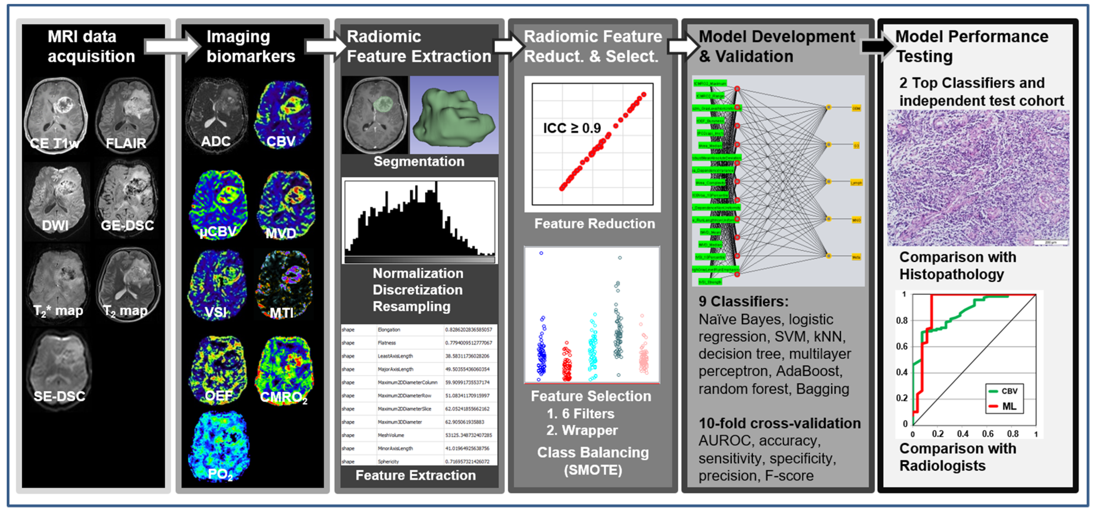
2. Materials and Methods
2.1. Ethics
2.2. Patients
2.3. MRI Data Acquisition
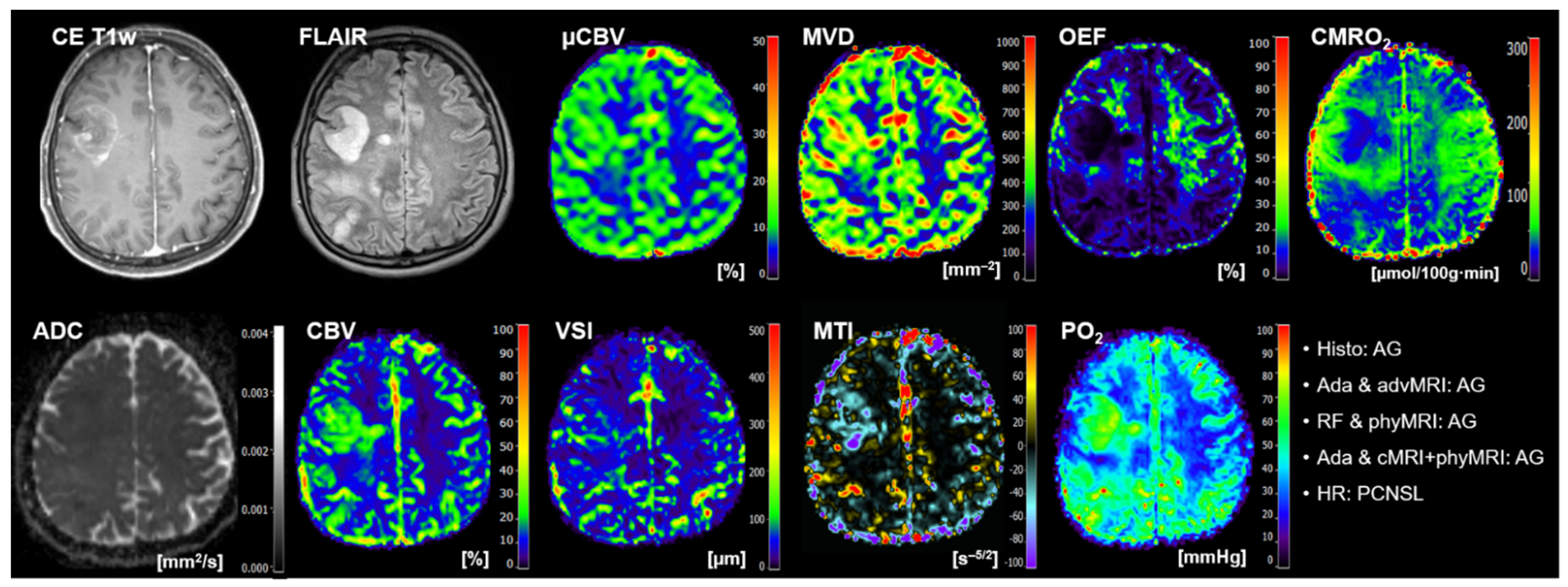
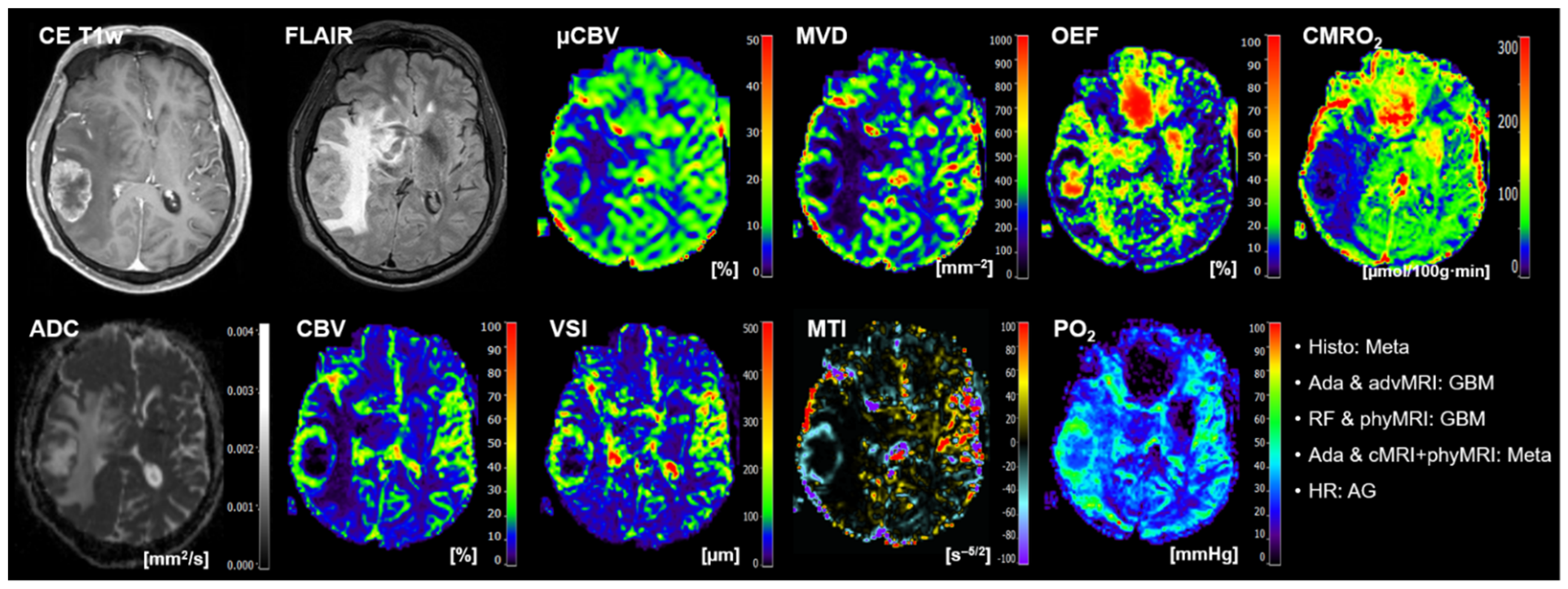
- The conventional anatomical MRI (cMRI) protocol for clinical routine diagnosis of brain tumors included, among others, an axial fluid-attenuated inversion recovery (FLAIR) sequence as well as a high-resolution contrast-enhanced T1-weighted (CE T1w) sequence.
- The advanced MRI (advMRI) protocol for clinical routine diagnosis of brain tumors was extended by axial diffusion-weighted imaging (DWI; b values 0 and 1000 s/mm2) sequence and a gradient echo dynamic susceptibility contrast (GE-DSC) perfusion MRI sequence, which was performed using 60 dynamic measurements during administration of 0.1 mmol/kg-bodyweight gadoterate-meglumine (Dotarem, Guerbet, Aulnay-Sous-Bois, France).
- The physiological MRI (phyMRI) protocol included the innovative MRI techniques of vascular architecture mapping (VAM) [31] for the assessment of microvascular architecture and neovascularization activity, as well as the quantitative blood-oxygenation-level-dependent (qBOLD) imaging approach [19,32] for assessment of tissue oxygen metabolism and tension. The VAM approach [33,34] additionally required a spin-echo DSC (SE-DSC) perfusion MRI sequence conducted with the same parameters and contrast agent injection protocol as described for the routine GE-DSC perfusion MRI. Details of our strategy to minimize adverse effects due to differences in time to first-pass peak and contrast-agent leakage, which could significantly affect the data evaluation, were previously described [33,34]. The qBOLD approach [19,32] additionally required a multi-echo GE sequence and a multi-echo SE sequence for the mapping of the transverse relaxation rates R2* (=1/T2*) and R2 (=1/T2), respectively. All phyMRI sequences for VAM and qBOLD were carried out with identical geometric parameters (voxel size, number of slices, etc.) and slice position as used for the routine GE-DSC perfusion sequence. The phyMRI protocol required seven minutes of extra scan time in total.
2.4. MRI Data Processing and Calculation of MRI Biomarker Maps
2.5. Radiomic Feature Extraction
- Fourteen shape features, which represent the three-dimensional size and shape of the segmented volume of interest (VOI, i.e., contrast-enhancing tumor and peritumoral edema). These features included elongation, flatness, least and major axis length, maximum 2D diameter of column, maximum 2D diameter of row, maximum 2D diameter of slice, maximum 3D diameter, mesh volume, minor axis length, sphericity, surface area, surface volume ratio, and voxel volume.
- Eighteen first-order features, which represent the distribution of gray values within an image, were calculated from the histogram of voxel intensities. These features included the 10th and 90th percentile, energy, entropy, interquartile range, kurtosis, maximum, mean absolute deviation, mean, median, minimum, range, robust mean absolute deviation, root mean squared, skewness, total energy, uniformity, and variance.
- Seventy-five texture features, which describe relationships between neighboring voxels with similar or dissimilar values. These features included the following 6 subcategories: (i) 24 gray-level co-occurrence matrix (GLCM) features characterizing how often pairs of voxels with specific intensity levels and spatial relationships occurred in an image [55]; (ii) 14 gray-level dependence matrix (GLDM) features representing the dependency of connected voxels to a center voxel [56]; (iii) 16 gray-level run-length matrix (GLRLM) features evaluating the length of consecutive pixels with the same gray level [57]; (iv) 16 gray-level size zone matrix (GLSZM) features quantifying the number of connected voxels that share the same intensity value [58]; and (v) 5 neighboring gray-tone difference matrix (NGTDM) features assessing differences between pixel values and neighbor average gray values [59]. Schematic representation of the extraction of first-order features, GLDM features, and NGTDM features is depicted in Figure S1 in the Supplementary Materials.
2.6. Radiomic Feature Reduction and Selection
2.7. Model Development and Validation
2.8. Model Performance Testing and Human Reading
3. Results
3.1. Patient Characteristics
- Seventy-seven patients (46%; 32 females; 45 males; mean age 63.2 ± 12.3 years; 31–84 years) had the diagnosis of a glioblastoma WHO grade 4;
- Seventeen patients (10%; 7 females; 10 males; mean age 49.9 ± 16.1 years; 21–73 years) had an anaplastic glioma WHO grade 3;
- Twenty-eight patients (17%; 18 females; 10 males; mean age 60.3 ± 13.2 years; 27–82 years) had a meningioma (15 patients WHO grade I, 12 patients WHO grade II; one patient WHO grade III);
- Sixteen patients (10%; 8 females; 8 males; mean age 69.8 ± 9.7 years; 55–92 years) had a PCNSL;
- Twenty-nine patients (17%; 16 females; 13 males; mean age 63.4 ± 9.3 years; 46–79 years) suffered from a brain metastasis that originated in twelve patients from lung cancer, in five patients from breast cancer, in four patients from a melanoma, in two patients each from esophageal or renal cancer, and in one patient each from fibrosarcoma, bladder cancer, pancreatic cancer, and colon cancer, respectively.
- Nine patients (45%; 4 females; 5 males; mean age 60.9 ± 18.5 years; 26–79 years) had a glioblastoma WHO grade 4;
- Three patients (15%; 2 females; 1 male; mean age 45.8 ± 19.8 years; 24–63 years) had an anaplastic glioma WHO grade 3;
- Three patients (15%; 1 female; 2 males; mean age 55.6 ± 16.2 years; 37–68 years) had a meningioma (1 patient WHO grade I and 2 patients WHO grade II);
- Five patients (25%; 4 females; 1 male; mean age 63.4 ± 4.3 years; 59–70 years) suffered from a brain metastasis that originated in two patients from lung cancer, and in one patient each from gastrointestinal cancer, bladder cancer, and breast cancer, respectively.
3.2. The Selected Radiomic Features
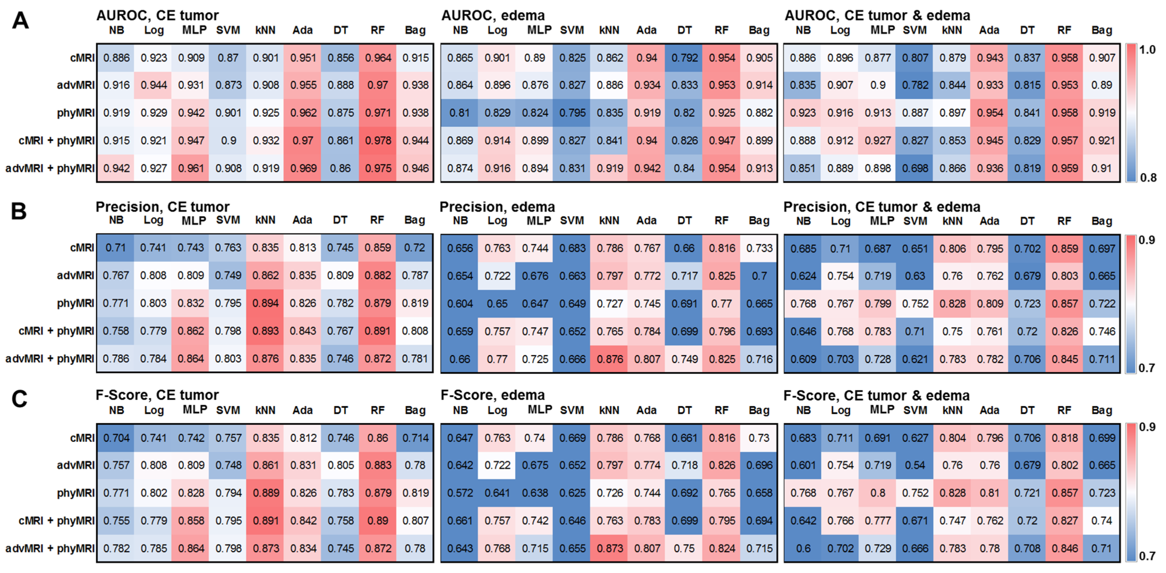
3.3. The Top ML Classifiers in the Learning/Validation Cohort
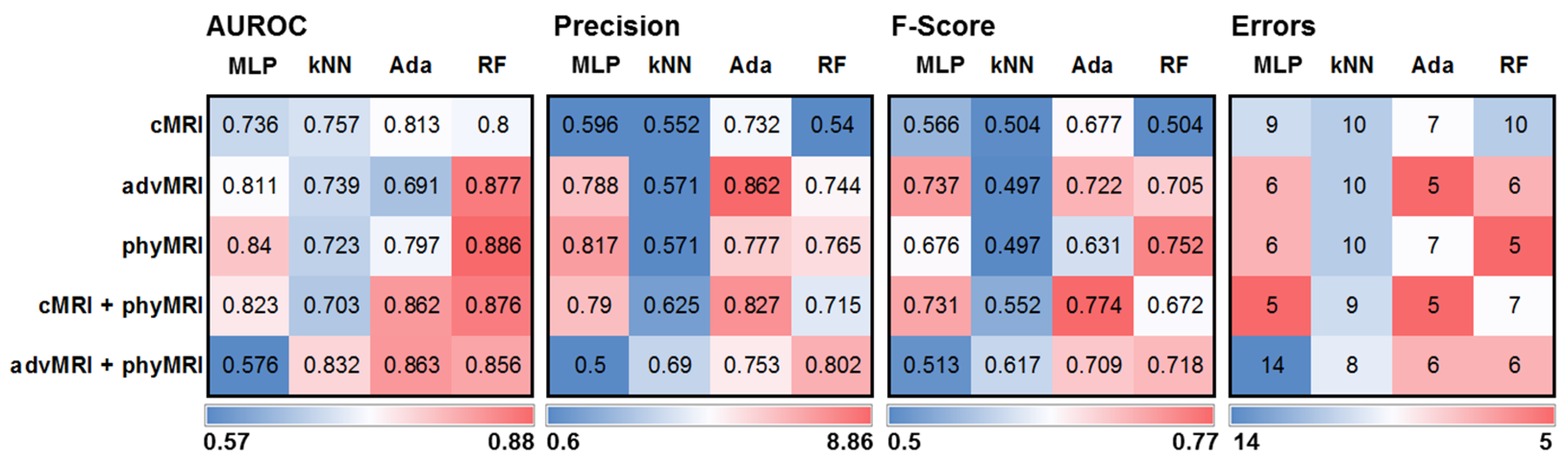
3.4. The Performance of the Selected Models in the Test Cohort
4. Discussion
5. Conclusions
Supplementary Materials
Author Contributions
Funding
Institutional Review Board Statement
Informed Consent Statement
Data Availability Statement
Conflicts of Interest
References
- Molinaro, A.M.; Taylor, J.W.; Wiencke, J.K.; Wrensch, M.R. Genetic and molecular epidemiology of adult diffuse glioma. Nat. Rev. Neurol. 2019, 15, 405–417. [Google Scholar] [CrossRef] [PubMed]
- Vigneswaran, K.; Neill, S.; Hadjipanayis, C.G. Beyond the World Health Organization grading of infiltrating gliomas: Advances in the molecular genetics of glioma classification. Ann. Transl. Med. 2015, 3, 95. [Google Scholar] [PubMed]
- Wen, P.Y.; Kesari, S. Malignant Gliomas in Adults. N. Engl. J. Med. 2008, 359, 492–507. [Google Scholar] [CrossRef] [PubMed] [Green Version]
- Hoffman, S.; Propp, J.M.; McCarthy, B.J. Temporal trends in incidence of primary brain tumors in the United States, 1985–1999. Neuro. Oncol. 2006, 8, 27–37. [Google Scholar] [CrossRef]
- Mendez, J.S.; Ostrom, Q.T.; Gittleman, H.; Kruchko, C.; DeAngelis, L.M.; Barnholtz-Sloan, J.S.; Grommes, C. The elderly left behind-changes in survival trends of primary central nervous system lymphoma over the past 4 decades. Neuro. Oncol. 2018, 20, 687–694. [Google Scholar] [CrossRef]
- Ostrom, Q.T.; McCulloh, C.; Chen, Y.; Devine, K.; Wolinsky, Y.; Davitkov, P.; Robbins, S.; Cherukuri, R.; Patel, A.; Gupta, R.; et al. Family History of Cancer in Benign Brain Tumor Subtypes Versus Gliomas. Front. Oncol. 2012, 2, 19. [Google Scholar] [CrossRef] [Green Version]
- Holleczek, B.; Zampella, D.; Urbschat, S.; Sahm, F.; von Deimling, A.; Oertel, J.; Ketter, R. Incidence, mortality and outcome of meningiomas: A population-based study from Germany. Cancer Epidemiol. 2019, 62, 101562. [Google Scholar] [CrossRef]
- Ranjan, T.; Abrey, L.E. Current management of metastatic brain disease. Neurotherapeutics 2009, 6, 598–603. [Google Scholar] [CrossRef] [Green Version]
- Abe, T.; Mizobuchi, Y.; Nakajima, K.; Otomi, Y.; Irahara, S.; Obama, Y.; Majigsuren, M.; Khashbat, D.; Kageji, T.; Nagahiro, S.; et al. Diagnosis of brain tumors using dynamic contrast-enhanced perfusion imaging with a short acquisition time. Springerplus 2015, 4, 88. [Google Scholar] [CrossRef] [Green Version]
- Mukundan, S.; Holder, C.; Olson, J.J. Neuroradiological assessment of newly diagnosed glioblastoma. J. Neurooncol. 2008, 89, 259–269. [Google Scholar] [CrossRef]
- Marko, N.F.; Weil, R.J.; Schroeder, J.L.; Lang, F.F.; Suki, D.; Sawaya, R.E. Extent of resection of glioblastoma revisited: Personalized survival modeling facilitates more accurate survival prediction and supports a maximum-safe-resection approach to surgery. J. Clin. Oncol. 2014, 32, 774–782. [Google Scholar] [CrossRef] [PubMed] [Green Version]
- Bataille, B.; Delwail, V.; Menet, E.; Vandermarcq, P.; Ingrand, P.; Wager, M.; Guy, G.; Lapierre, F. Primary intracerebral malignant lymphoma: Report of 248 cases. J. Neurosurg. 2000, 92, 261–266. [Google Scholar] [CrossRef] [PubMed]
- Weller, M.; van den Bent, M.; Hopkins, K.; Tonn, J.C.; Stupp, R.; Falini, A.; Cohen-Jonathan-Moyal, E.; Frappaz, D.; Henriksson, R.; Balana, C.; et al. EANO guideline for the diagnosis and treatment of anaplastic gliomas and glioblastoma. Lancet Oncol. 2014, 15, e395–e403. [Google Scholar] [CrossRef] [Green Version]
- Pasricha, S.; Gupta, A.; Gawande, J.; Trivedi, P.; Patel, D. Primary central nervous system lymphoma: A study of clinicopathological features and trend in western India. Indian J. Cancer 2011, 48, 199–203. [Google Scholar] [CrossRef]
- Olivero, W.C.; Lister, J.R.; Elwood, P.W. The natural history and growth rate of asymptomatic meningiomas: A review of 60 patients. J. Neurosurg. 1995, 83, 222–224. [Google Scholar] [CrossRef]
- Gaudy-Marqueste, C.; Carron, R.; Delsanti, C.; Loundou, A.; Monestier, S.; Archier, E.; Richard, M.A.; Regis, J.; Grob, J.J. On demand Gamma-Knife strategy can be safely combined with BRAF inhibitors for the treatment of melanoma brain metastases. Ann. Oncol. Off. J. Eur. Soc. Med. Oncol. 2014, 25, 2086–2091. [Google Scholar] [CrossRef]
- Hardee, M.E.; Zagzag, D. Mechanisms of glioma-associated neovascularization. Am. J. Pathol. 2012, 181, 1126–1141. [Google Scholar] [CrossRef] [Green Version]
- Stadlbauer, A.; Kinfe, T.M.; Eyüpoglu, I.; Zimmermann, M.; Kitzwögerer, M.; Podar, K.; Buchfelder, M.; Heinz, G.; Oberndorfer, S.; Marhold, F. Tissue Hypoxia and Alterations in Microvascular Architecture Predict Glioblastoma Recurrence in Humans. Clin. Cancer Res. 2021, 27, 1641–1649. [Google Scholar] [CrossRef]
- Stadlbauer, A.; Zimmermann, M.; Doerfler, A.; Oberndorfer, S.; Buchfelder, M.; Coras, R.; Kitzwögerer, M.; Roessler, K. Intratumoral heterogeneity of oxygen metabolism and neovascularization uncovers 2 survival-relevant subgroups of IDH1 wild-type glioblastoma. Neuro. Oncol. 2018, 20, 1536–1546. [Google Scholar] [CrossRef] [Green Version]
- Stadlbauer, A.; Zimmermann, M.; Bennani-Baiti, B.; Helbich, T.H.; Baltzer, P.; Clauser, P.; Kapetas, P.; Bago-Horvath, Z.; Pinker, K. Development of a Non-invasive Assessment of Hypoxia and Neovascularization with Magnetic Resonance Imaging in Benign and Malignant Breast Tumors: Initial Results. Mol. Imaging Biol. 2019, 21, 758–770. [Google Scholar] [CrossRef] [Green Version]
- Bennani-Baiti, B.; Pinker, K.; Zimmermann, M.; Helbich, T.H.; Baltzer, P.A.; Clauser, P.; Kapetas, P.; Bago-Horvath, Z.; Stadlbauer, A. Non-Invasive Assessment of Hypoxia and Neovascularization with MRI for Identification of Aggressive Breast Cancer. Cancers 2020, 12, 2024. [Google Scholar] [CrossRef] [PubMed]
- Boxerman, J.L.; Hamberg, L.M.; Rosen, B.R.; Weisskoff, R.M. MR contrast due to intravascular magnetic susceptibility perturbations. Magn. Reson. Med. 1995, 34, 555–566. [Google Scholar] [CrossRef] [PubMed]
- Christen, T.; Schmiedeskamp, H.; Straka, M.; Bammer, R.; Zaharchuk, G. Measuring brain oxygenation in humans using a multiparametric quantitative blood oxygenation level dependent MRI approach. Magn. Reson. Med. 2012, 68, 905–911. [Google Scholar] [CrossRef] [PubMed]
- Cai, X.; Li, X.; Razmjooy, N.; Ghadimi, N. Breast Cancer Diagnosis by Convolutional Neural Network and Advanced Thermal Exchange Optimization Algorithm. Comput. Math. Methods Med. 2021, 2021, 5595180. [Google Scholar] [CrossRef]
- Van der Laak, J.; Litjens, G.; Ciompi, F. Deep learning in histopathology: The path to the clinic. Nat. Med. 2021, 27, 775–784. [Google Scholar] [CrossRef]
- Stacke, K.; Eilertsen, G.; Unger, J.; Lundstrom, C. Measuring Domain Shift for Deep Learning in Histopathology. IEEE J. Biomed. Health Inform. 2021, 25, 325–336. [Google Scholar] [CrossRef]
- Jimenez-del-Toro, O.; Otálora, S.; Andersson, M.; Eurén, K.; Hedlund, M.; Rousson, M.; Müller, H.; Atzori, M. Analysis of Histopathology Images. In Biomedical Texture Analysis; Elsevier: Amsterdam, The Netherlands, 2017; pp. 281–314. ISBN 9780128121337. [Google Scholar]
- Hu, A.; Razmjooy, N. Brain tumor diagnosis based on metaheuristics and deep learning. Int. J. Imaging Syst. Technol. 2021, 31, 657–669. [Google Scholar] [CrossRef]
- Gillies, R.J.; Kinahan, P.E.; Hricak, H. Radiomics: Images Are More than Pictures, They Are Data. Radiology 2016, 278, 563–577. [Google Scholar] [CrossRef] [Green Version]
- Lambin, P.; Leijenaar, R.T.H.; Deist, T.M.; Peerlings, J.; de Jong, E.E.C.; van Timmeren, J.; Sanduleanu, S.; Larue, R.T.H.M.; Even, A.J.G.; Jochems, A.; et al. Radiomics: The bridge between medical imaging and personalized medicine. Nat. Rev. Clin. Oncol. 2017, 14, 749–762. [Google Scholar] [CrossRef]
- Stadlbauer, A.; Eyüpoglu, I.; Buchfelder, M.; Dörfler, A.; Zimmermann, M.; Heinz, G.; Oberndorfer, S. Vascular architecture mapping for early detection of glioblastoma recurrence. Neurosurg. Focus 2019, 47, E14. [Google Scholar] [CrossRef] [Green Version]
- Stadlbauer, A.; Zimmermann, M.; Kitzwögerer, M.; Oberndorfer, S.; Rössler, K.; Dörfler, A.; Buchfelder, M.; Heinz, G. MR Imaging—Derived Oxygen Metabolism and Neovascularization Characterization for Grading and IDH Gene Mutation Detection of Gliomas. Radiology 2017, 283, 799–809. [Google Scholar] [CrossRef] [PubMed] [Green Version]
- Stadlbauer, A.; Zimmermann, M.; Heinz, G.; Oberndorfer, S.; Doerfler, A.; Buchfelder, M.; Rössler, K. Magnetic resonance imaging biomarkers for clinical routine assessment of microvascular architecture in glioma. J. Cereb. Blood Flow Metab. 2017, 37, 632–643. [Google Scholar] [CrossRef] [PubMed] [Green Version]
- Stadlbauer, A.; Zimmermann, M.; Oberndorfer, S.; Doerfler, A.; Buchfelder, M.; Heinz, G.; Roessler, K. Vascular Hysteresis Loops and Vascular Architecture Mapping in Patients with Glioblastoma treated with Antiangiogenic Therapy. Sci. Rep. 2017, 7, 8508. [Google Scholar] [CrossRef] [PubMed] [Green Version]
- Smith, A.M.; Grandin, C.B.; Duprez, T.; Mataigne, F.; Cosnard, G. Whole brain quantitative CBF, CBV, and MTT measurements using MRI bolus tracking: Implementation and application to data acquired from hyperacute stroke patients. J. Magn. Reson. Imaging 2000, 12, 400–410. [Google Scholar] [CrossRef]
- Bjørnerud, A.; Emblem, K.E. A Fully Automated Method for Quantitative Cerebral Hemodynamic Analysis Using DSC–MRI. J. Cereb. Blood Flow Metab. 2010, 30, 1066–1078. [Google Scholar] [CrossRef] [Green Version]
- Boxerman, J.L.; Prah, D.E.; Paulson, E.S.; Machan, J.T.; Bedekar, D.; Schmainda, K.M. The Role of Preload and Leakage Correction in Gadolinium-Based Cerebral Blood Volume Estimation Determined by Comparison with MION as a Criterion Standard. Am. J. Neuroradiol. 2012, 33, 1081–1087. [Google Scholar] [CrossRef] [Green Version]
- Boxerman, J.L.; Schmainda, K.M.; Weisskoff, R.M. Relative cerebral blood volume maps corrected for contrast agent extravasation significantly correlate with glioma tumor grade, whereas uncorrected maps do not. AJNR. Am. J. Neuroradiol. 2006, 27, 859–867. [Google Scholar]
- Ducreux, D.; Buvat, I.; Meder, J.F.; Mikulis, D.; Crawley, A.; Fredy, D.; TerBrugge, K.; Lasjaunias, P.; Bittoun, J. Perfusion-weighted MR imaging studies in brain hypervascular diseases: Comparison of arterial input function extractions for perfusion measurement. AJNR. Am. J. Neuroradiol. 2006, 27, 1059–1069. [Google Scholar]
- Xu, C.; Kiselev, V.G.; Möller, H.E.; Fiebach, J.B. Dynamic hysteresis between gradient echo and spin echo attenuations in dynamic susceptibility contrast imaging. Magn. Reson. Med. 2013, 69, 981–991. [Google Scholar] [CrossRef]
- Jensen, J.H.; Lu, H.; Inglese, M. Microvessel density estimation in the human brain by means of dynamic contrast-enhanced echo-planar imaging. Magn. Reson. Med. 2006, 56, 1145–1150. [Google Scholar] [CrossRef]
- Emblem, K.E.; Mouridsen, K.; Bjornerud, A.; Farrar, C.T.; Jennings, D.; Borra, R.J.H.; Wen, P.Y.; Ivy, P.; Batchelor, T.T.; Rosen, B.R.; et al. Vessel architectural imaging identifies cancer patient responders to anti-angiogenic therapy. Nat. Med. 2013, 19, 1178–1183. [Google Scholar] [CrossRef] [PubMed]
- Preibisch, C.; Volz, S.; Anti, S.; Deichmann, R. Exponential excitation pulses for improved water content mapping in the presence of background gradients. Magn. Reson. Med. 2008, 60, 908–916. [Google Scholar] [CrossRef] [PubMed]
- Prasloski, T.; Mädler, B.; Xiang, Q.-S.; MacKay, A.; Jones, C. Applications of stimulated echo correction to multicomponent T 2 analysis. Magn. Reson. Med. 2012, 67, 1803–1814. [Google Scholar] [CrossRef] [PubMed]
- Kennan, R.P.; Zhong, J.; Gore, J.C. Intravascular susceptibility contrast mechanisms in tissues. Magn. Reson. Med. 1994, 31, 9–21. [Google Scholar] [CrossRef]
- Vafaee, M.S.; Vang, K.; Bergersen, L.H.; Gjedde, A. Oxygen Consumption and Blood Flow Coupling in Human Motor Cortex during Intense Finger Tapping: Implication for a Role of Lactate. J. Cereb. Blood Flow Metab. 2012, 32, 1859–1868. [Google Scholar] [CrossRef] [Green Version]
- Gjedde, A. Cerebral Blood Flow Change in Arterial Hypoxemia Is Consistent with Negligible Oxygen Tension in Brain Mitochondria. Neuroimage 2002, 17, 1876–1881. [Google Scholar] [CrossRef]
- Vafaee, M.S.; Gjedde, A. Model of Blood—Brain Transfer of Oxygen Explains Nonlinear Flow-Metabolism Coupling During Stimulation of Visual Cortex. J. Cereb. Blood Flow Metab. 2000, 20, 747–754. [Google Scholar] [CrossRef] [Green Version]
- Li, Z.; Mao, Y.; Li, H.; Yu, G.; Wan, H.; Li, B. Differentiating brain metastases from different pathological types of lung cancers using texture analysis of T1 postcontrast MR. Magn. Reson. Med. 2016, 76, 1410–1419. [Google Scholar] [CrossRef]
- Carré, A.; Klausner, G.; Edjlali, M.; Lerousseau, M.; Briend-Diop, J.; Sun, R.; Ammari, S.; Reuzé, S.; Alvarez Andres, E.; Estienne, T.; et al. Standardization of brain MR images across machines and protocols: Bridging the gap for MRI-based radiomics. Sci. Rep. 2020, 10, 12340. [Google Scholar] [CrossRef]
- Collewet, G.; Strzelecki, M.; Mariette, F. Influence of MRI acquisition protocols and image intensity normalization methods on texture classification. Magn. Reson. Imaging 2004, 22, 81–91. [Google Scholar] [CrossRef]
- Shafiq-Ul-Hassan, M.; Zhang, G.G.; Latifi, K.; Ullah, G.; Hunt, D.C.; Balagurunathan, Y.; Abdalah, M.A.; Schabath, M.B.; Goldgof, D.G.; Mackin, D.; et al. Intrinsic dependencies of CT radiomic features on voxel size and number of gray levels. Med. Phys. 2017, 44, 1050–1062. [Google Scholar] [CrossRef] [PubMed]
- Van Griethuysen, J.J.M.; Fedorov, A.; Parmar, C.; Hosny, A.; Aucoin, N.; Narayan, V.; Beets-Tan, R.G.H.; Fillion-Robin, J.-C.; Pieper, S.; Aerts, H.J.W.L. Computational Radiomics System to Decode the Radiographic Phenotype. Cancer Res. 2017, 77, e104–e107. [Google Scholar] [CrossRef] [PubMed] [Green Version]
- Zwanenburg, A.; Vallières, M.; Abdalah, M.A.; Aerts, H.J.W.L.; Andrearczyk, V.; Apte, A.; Ashrafinia, S.; Bakas, S.; Beukinga, R.J.; Boellaard, R.; et al. The Image Biomarker Standardization Initiative: Standardized Quantitative Radiomics for High-Throughput Image-based Phenotyping. Radiology 2020, 295, 328–338. [Google Scholar] [CrossRef] [PubMed] [Green Version]
- Haralick, R.M.; Shanmugam, K.; Dinstein, I. Textural Features for Image Classification. IEEE Trans. Syst. Man Cybern 1973, SMC-3, 610–621. [Google Scholar] [CrossRef] [Green Version]
- Sun, C.; Wee, W.G. Neighboring gray level dependence matrix for texture classification. Comput. Vis. Graph. Image Process. 1983, 23, 341–352. [Google Scholar] [CrossRef]
- Galloway, M.M. Texture analysis using gray level run lengths. Comput. Graph. Image Process. 1975, 4, 172–179. [Google Scholar] [CrossRef]
- Thibault, G.; Fertil, B.; Navarro, C.; Pereira, S.; Cau, P.; Levy, N.; Sequeira, J.; Mari, J.-L. Shape and Texture Indexes Application to Cell Nuclei Classification. Int. J. Pattern Recognit. Artif. Intell. 2013, 27, 1357002. [Google Scholar] [CrossRef]
- Amadasun, M.; King, R. Textural features corresponding to textural properties. IEEE Trans. Syst. Man Cybern. 1989, 19, 1264–1274. [Google Scholar] [CrossRef]
- Baessler, B.; Nestler, T.; Pinto dos Santos, D.; Paffenholz, P.; Zeuch, V.; Pfister, D.; Maintz, D.; Heidenreich, A. Radiomics allows for detection of benign and malignant histopathology in patients with metastatic testicular germ cell tumors prior to post-chemotherapy retroperitoneal lymph node dissection. Eur. Radiol. 2020, 30, 2334–2345. [Google Scholar] [CrossRef]
- Moradmand, H.; Aghamiri, S.M.R.; Ghaderi, R. Impact of image preprocessing methods on reproducibility of radiomic features in multimodal magnetic resonance imaging in glioblastoma. J. Appl. Clin. Med. Phys. 2020, 21, 179–190. [Google Scholar] [CrossRef]
- Mannil, M.; Burgstaller, J.M.; Held, U.; Farshad, M.; Guggenberger, R. Correlation of texture analysis of paraspinal musculature on MRI with different clinical endpoints: Lumbar Stenosis Outcome Study (LSOS). Eur. Radiol. 2019, 29, 22–30. [Google Scholar] [CrossRef]
- Zacharaki, E.I.; Wang, S.; Chawla, S.; Soo Yoo, D.; Wolf, R.; Melhem, E.R.; Davatzikos, C. Classification of brain tumor type and grade using MRI texture and shape in a machine learning scheme. Magn. Reson. Med. 2009, 62, 1609–1618. [Google Scholar] [CrossRef] [PubMed] [Green Version]
- Chawla, N.V.; Bowyer, K.W.; Hall, L.O.; Kegelmeyer, W.P. SMOTE: Synthetic Minority Over-sampling Technique. J. Artif. Intell. Res. 2011, 16, 321–357. [Google Scholar] [CrossRef]
- Payabvash, S.; Aboian, M.; Tihan, T.; Cha, S. Machine Learning Decision Tree Models for Differentiation of Posterior Fossa Tumors Using Diffusion Histogram Analysis and Structural MRI Findings. Front. Oncol. 2020, 10, 1–15. [Google Scholar] [CrossRef]
- Zacharaki, E.I.; Kanas, V.G.; Davatzikos, C. Investigating machine learning techniques for MRI-based classification of brain neoplasms. Int. J. Comput. Assist. Radiol. Surg. 2011, 6, 821–828. [Google Scholar] [CrossRef] [Green Version]
- Bradley, A.P. The use of the area under the ROC curve in the evaluation of machine learning algorithms. Pattern Recognit. 1997, 30, 1145–1159. [Google Scholar] [CrossRef] [Green Version]
- Wiestler, B.; Kluge, A.; Lukas, M.; Gempt, J.; Ringel, F.; Schlegel, J.; Meyer, B.; Zimmer, C.; Förster, S.; Pyka, T.; et al. Multiparametric MRI-based differentiation of WHO grade II/III glioma and WHO grade IV glioblastoma. Sci. Rep. 2016, 6, 35142. [Google Scholar] [CrossRef]
- Cao, H.; Erson-Omay, E.Z.; Li, X.; Günel, M.; Moliterno, J.; Fulbright, R.K. A quantitative model based on clinically relevant MRI features differentiates lower grade gliomas and glioblastoma. Eur. Radiol. 2020, 30, 3073–3082. [Google Scholar] [CrossRef]
- Zhang, X.; Yan, L.-F.; Hu, Y.-C.; Li, G.; Yang, Y.; Han, Y.; Sun, Y.-Z.; Liu, Z.-C.; Tian, Q.; Han, Z.-Y.; et al. Optimizing a machine learning based glioma grading system using multi-parametric MRI histogram and texture features. Oncotarget 2017, 8, 47816–47830. [Google Scholar] [CrossRef]
- Kim, M.; Jung, S.Y.; Park, J.E.; Jo, Y.; Park, S.Y.; Nam, S.J.; Kim, J.H.; Kim, H.S. Diffusion- and perfusion-weighted MRI radiomics model may predict isocitrate dehydrogenase (IDH) mutation and tumor aggressiveness in diffuse lower grade glioma. Eur. Radiol. 2020, 30, 2142–2151. [Google Scholar] [CrossRef]
- Ren, Y.; Zhang, X.; Rui, W.; Pang, H.; Qiu, T.; Wang, J.; Xie, Q.; Jin, T.; Zhang, H.; Chen, H.; et al. Noninvasive Prediction of IDH1 Mutation and ATRX Expression Loss in Low-Grade Gliomas Using Multiparametric MR Radiomic Features. J. Magn. Reson. Imaging 2019, 49, 808–817. [Google Scholar] [CrossRef] [PubMed]
- Tatekawa, H.; Hagiwara, A.; Uetani, H.; Bahri, S.; Raymond, C.; Lai, A.; Cloughesy, T.F.; Nghiemphu, P.L.; Liau, L.M.; Pope, W.B.; et al. Differentiating IDH status in human gliomas using machine learning and multiparametric MR/PET. Cancer Imaging 2021, 21, 27. [Google Scholar] [CrossRef] [PubMed]
- Sudre, C.H.; Panovska-Griffiths, J.; Sanverdi, E.; Brandner, S.; Katsaros, V.K.; Stranjalis, G.; Pizzini, F.B.; Ghimenton, C.; Surlan-Popovic, K.; Avsenik, J.; et al. Machine learning assisted DSC-MRI radiomics as a tool for glioma classification by grade and mutation status. BMC Med. Inform. Decis. Mak. 2020, 20, 149. [Google Scholar] [CrossRef]
- Tateishi, M.; Nakaura, T.; Kitajima, M.; Uetani, H.; Nakagawa, M.; Inoue, T.; Kuroda, J.-I.; Mukasa, A.; Yamashita, Y. An initial experience of machine learning based on multi-sequence texture parameters in magnetic resonance imaging to differentiate glioblastoma from brain metastases. J. Neurol. Sci. 2020, 410, 116514. [Google Scholar] [CrossRef]
- Sartoretti, E.; Sartoretti, T.; Wyss, M.; Reischauer, C.; van Smoorenburg, L.; Binkert, C.A.; Sartoretti-Schefer, S.; Mannil, M. Amide proton transfer weighted (APTw) imaging based radiomics allows for the differentiation of gliomas from metastases. Sci. Rep. 2021, 11, 5506. [Google Scholar] [CrossRef]
- Qian, Z.; Li, Y.; Wang, Y.; Li, L.; Li, R.; Wang, K.; Li, S.; Tang, K.; Zhang, C.; Fan, X.; et al. Differentiation of glioblastoma from solitary brain metastases using radiomic machine-learning classifiers. Cancer Lett. 2019, 451, 128–135. [Google Scholar] [CrossRef]
- Bae, S.; An, C.; Ahn, S.S.; Kim, H.; Han, K.; Kim, S.W.; Park, J.E.; Kim, H.S.; Lee, S.-K. Robust performance of deep learning for distinguishing glioblastoma from single brain metastasis using radiomic features: Model development and validation. Sci. Rep. 2020, 10, 12110. [Google Scholar] [CrossRef]
- Ortiz-Ramón, R.; Ruiz-España, S.; Mollá-Olmos, E.; Moratal, D. Glioblastomas and brain metastases differentiation following an MRI texture analysis-based radiomics approach. Phys. Med. 2020, 76, 44–54. [Google Scholar] [CrossRef]
- Tian, Z.; Chen, C.; Fan, Y.; Ou, X.; Wang, J.; Ma, X.; Xu, J. Glioblastoma and Anaplastic Astrocytoma: Differentiation Using MRI Texture Analysis. Front. Oncol. 2019, 9, 876. [Google Scholar] [CrossRef]
- Qin, J.; Li, Y.; Liang, D.; Zhang, Y.; Yao, W. Histogram analysis of absolute cerebral blood volume map can distinguish glioblastoma from solitary brain metastasis. Med. (Baltim.) 2019, 98, e17515. [Google Scholar] [CrossRef]
- Nakagawa, M.; Nakaura, T.; Namimoto, T.; Kitajima, M.; Uetani, H.; Tateishi, M.; Oda, S.; Utsunomiya, D.; Makino, K.; Nakamura, H.; et al. Machine learning based on multi-parametric magnetic resonance imaging to differentiate glioblastoma multiforme from primary cerebral nervous system lymphoma. Eur. J. Radiol. 2018, 108, 147–154. [Google Scholar] [CrossRef] [PubMed]
- Swinburne, N.C.; Schefflein, J.; Sakai, Y.; Oermann, E.K.; Titano, J.J.; Chen, I.; Tadayon, S.; Aggarwal, A.; Doshi, A.; Nael, K. Machine learning for semiautomated classification of glioblastoma, brain metastasis and central nervous system lymphoma using magnetic resonance advanced imaging. Ann. Transl. Med. 2019, 7, 232. [Google Scholar] [CrossRef] [PubMed]
- Ahmad, M.; Qadri, S.F.; Qadri, S.; Saeed, I.A.; Zareen, S.S.; Iqbal, Z.; Alabrah, A.; Alaghbari, H.M.; Mizanur Rahman, S.M. A Lightweight Convolutional Neural Network Model for Liver Segmentation in Medical Diagnosis. Comput. Intell. Neurosci. 2022, 2022, 7954333. [Google Scholar] [CrossRef]
- Qadri, S.F.; Shen, L.; Ahmad, M.; Qadri, S.; Zareen, S.S.; Akbar, M.A. SVseg: Stacked Sparse Autoencoder-Based Patch Classification Modeling for Vertebrae Segmentation. Mathematics 2022, 10, 796. [Google Scholar] [CrossRef]
- Lu, L.; Dercle, L.; Zhao, B.; Schwartz, L.H. Deep learning for the prediction of early on-treatment response in metastatic colorectal cancer from serial medical imaging. Nat. Commun. 2021, 12, 6654. [Google Scholar] [CrossRef]


| Value | advMRI Maps | phyMRI Maps | |||||||
|---|---|---|---|---|---|---|---|---|---|
| ADC | CBV | µCBV | MVD | VSI | MTI | OEF | CMRO2 | PO2 | |
| range | [0, 3] | [0, 100] | [0.30] | [0, 2000] | [0, 500] | [−1000, 1000] | [0, 100] | [0, 1000] | [0, 200] |
| unit | mm2/s | % | % | mm−2 | µm | s−2/5 | % | µmol/100 g × min | mmHg |
| bin size | 0.05 | 1.5 | 0.5 | 30 | 8 | 30 | 1.5 | 15 | 3 |
| bins | 60 | 67 | 60 | 67 | 63 | 67 | 67 | 67 | 67 |
| Caption | NB | Log | MP | SVM | kNN | Ada | DT | RF | Bag | |
|---|---|---|---|---|---|---|---|---|---|---|
| cMRI | CE T1w | 9 | 21 | 16 | 23 | 10 | 15 | 11 | 14 | 8 |
| FLAIR | 1 | 1 | 0 | 1 | 1 | 1 | 0 | 1 | 0 | |
| total | 10 | 22 | 16 | 24 | 11 | 16 | 11 | 15 | 8 | |
| advMRI | CE T1w | 10 | 6 | 6 | 10 | 4 | 4 | 4 | 7 | 5 |
| FLAIR | 0 | 0 | 0 | 0 | 0 | 0 | 0 | 0 | 0 | |
| ADC | 2 | 1 | 2 | 2 | 1 | 1 | 1 | 1 | 1 | |
| CBV | 5 | 5 | 7 | 4 | 9 | 4 | 3 | 11 | 2 | |
| total | 17 | 12 | 15 | 16 | 14 | 9 | 8 | 19 | 8 | |
| phyMRI | CMRO2 | 3 | 2 | 3 | 4 | 1 | 3 | 2 | 2 | 1 |
| OEF | 2 | 2 | 2 | 1 | 0 | 2 | 0 | 2 | 3 | |
| PO2 | 1 | 1 | 0 | 1 | 0 | 2 | 0 | 1 | 1 | |
| MIT | 2 | 2 | 2 | 3 | 6 | 2 | 2 | 4 | 3 | |
| µCBV | 1 | 2 | 2 | 3 | 0 | 0 | 0 | 3 | 0 | |
| MVD | 5 | 3 | 1 | 4 | 3 | 4 | 5 | 2 | 2 | |
| VSI | 5 | 3 | 3 | 4 | 3 | 2 | 3 | 3 | 3 | |
| total | 19 | 15 | 13 | 20 | 13 | 15 | 12 | 17 | 13 | |
| cMRI + phyMRI | CE T1w | 5 | 11 | 20 | 16 | 11 | 10 | 9 | 9 | 6 |
| FLAIR | 0 | 0 | 0 | 0 | 0 | 0 | 0 | 0 | 0 | |
| CMRO2 | 2 | 2 | 2 | 3 | 3 | 1 | 1 | 1 | 1 | |
| OEF | 2 | 1 | 0 | 1 | 1 | 1 | 1 | 2 | 1 | |
| PO2 | 0 | 0 | 0 | 0 | 0 | 0 | 0 | 0 | 0 | |
| MIT | 1 | 2 | 5 | 5 | 3 | 1 | 1 | 3 | 3 | |
| µCBV | 1 | 2 | 1 | 1 | 1 | 0 | 0 | 0 | 2 | |
| MVD | 0 | 1 | 1 | 2 | 2 | 3 | 3 | 2 | 0 | |
| VSI | 3 | 2 | 4 | 3 | 4 | 3 | 3 | 5 | 3 | |
| total | 14 | 21 | 33 | 31 | 25 | 19 | 18 | 22 | 16 | |
| advMRI + phyMRI | CE T1w | 8 | 8 | 12 | 13 | 5 | 4 | 6 | 6 | 9 |
| FLAIR | 0 | 0 | 0 | 0 | 0 | 0 | 0 | 0 | 0 | |
| ADC | 0 | 0 | 0 | 0 | 0 | 0 | 0 | 0 | 0 | |
| CBV | 8 | 4 | 13 | 8 | 3 | 6 | 3 | 7 | 8 | |
| CMRO2 | 1 | 0 | 1 | 1 | 0 | 0 | 1 | 1 | 1 | |
| OEF | 1 | 0 | 0 | 1 | 0 | 1 | 0 | 0 | 0 | |
| PO2 | 0 | 0 | 1 | 0 | 0 | 0 | 0 | 0 | 0 | |
| MIT | 1 | 2 | 3 | 4 | 2 | 1 | 1 | 1 | 1 | |
| µCBV | 1 | 1 | 1 | 0 | 1 | 0 | 0 | 0 | 1 | |
| MVD | 1 | 0 | 1 | 1 | 0 | 0 | 0 | 0 | 0 | |
| VSI | 3 | 3 | 4 | 4 | 1 | 1 | 1 | 2 | 2 | |
| total | 24 | 18 | 36 | 32 | 12 | 13 | 12 | 17 | 22 |
| Caption | Accuracy | Sensitivity | Specificity | Precision | F-Score | AUROC | |
|---|---|---|---|---|---|---|---|
| RF | cMRI | 0.944 | 0.867 | 0.965 | 0.859 | 0.860 | 0.964 |
| advMRI | 0.953 | 0.889 | 0.970 | 0.882 | 0.883 | 0.97 | |
| phyMRI | 0.951 | 0.887 | 0.970 | 0.879 | 0.879 | 0.971 | |
| cMRI + phyMRI | 0.956 | 0.897 | 0.973 | 0.891 | 0.890 | 0.978 | |
| advMRI + phyMRI | 0.948 | 0.878 | 0.968 | 0.872 | 0.872 | 0.975 | |
| Ada | cMRI | 0.924 | 0.817 | 0.952 | 0.813 | 0.812 | 0.951 |
| advMRI | 0.931 | 0.837 | 0.957 | 0.835 | 0.831 | 0.955 | |
| phyMRI | 0.929 | 0.831 | 0.955 | 0.826 | 0.826 | 0.962 | |
| cMRI + phyMRI | 0.936 | 0.847 | 0.960 | 0.843 | 0.842 | 0.97 | |
| advMRI + phyMRI | 0.934 | 0.842 | 0.959 | 0.835 | 0.834 | 0.969 | |
| kNN | cMRI | 0.934 | 0.842 | 0.959 | 0.835 | 0.835 | 0.901 |
| advMRI | 0.944 | 0.867 | 0.965 | 0.862 | 0.861 | 0.908 | |
| phyMRI | 0.956 | 0.898 | 0.973 | 0.894 | 0.889 | 0.925 | |
| cMRI + phyMRI | 0.956 | 0.897 | 0.973 | 0.893 | 0.891 | 0.932 | |
| advMRI + phyMRI | 0.949 | 0.881 | 0.969 | 0.876 | 0.873 | 0.919 | |
| MP | cMRI | 0.897 | 0.748 | 0.935 | 0.743 | 0.742 | 0.909 |
| advMRI | 0.923 | 0.814 | 0.952 | 0.809 | 0.809 | 0.931 | |
| phyMRI | 0.931 | 0.834 | 0.957 | 0.832 | 0.828 | 0.942 | |
| cMRI + phyMRI | 0.943 | 0.864 | 0.965 | 0.862 | 0.858 | 0.947 | |
| advMRI + phyMRI | 0.945 | 0.869 | 0.965 | 0.864 | 0.864 | 0.961 | |
| Human Reading | 0.846 | 0.739 | 0.927 | 0.767 | 0.708 | 0.808 | |
| Caption | Accuracy | Sensitivity | Specificity | Precision | F-Score | AUROC | Errors | |
|---|---|---|---|---|---|---|---|---|
| Ada | cMRI | 0.815 | 0.650 | 0.852 | 0.732 | 0.677 | 0.813 | 7 |
| Ada | advMRI | 0.853 | 0.750 | 0.836 | 0.862 | 0.722 | 0.691 | 5 |
| RF | phyMRI | 0.830 | 0.750 | 0.844 | 0.765 | 0.752 | 0.886 | 5 |
| Ada | cMRI + phyMRI | 0.875 | 0.750 | 0.902 | 0.827 | 0.774 | 0.862 | 5 |
| RF | advMRI + phyMRI | 0.843 | 0.700 | 0.860 | 0.802 | 0.718 | 0.863 | 6 |
| Human Reading | 0.850 | 0.767 | 0.925 | 0.798 | 0.740 | 0.813 | 6 | |
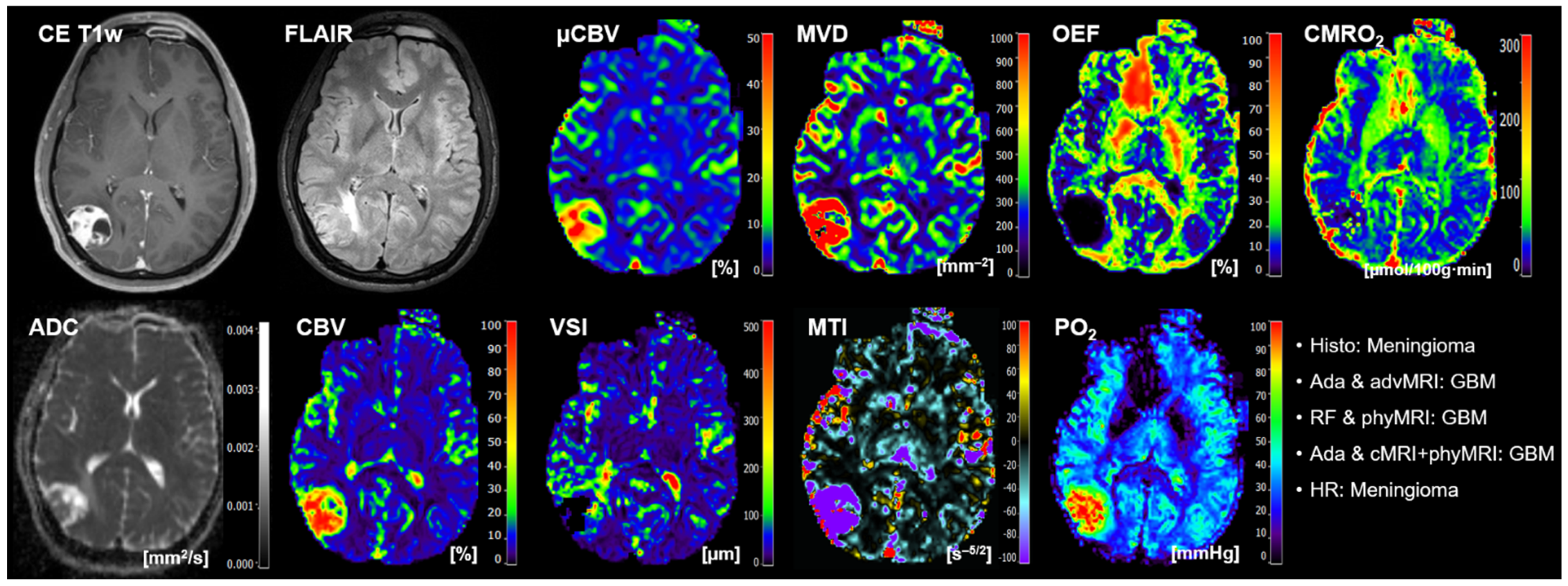
| ID | Histology | AdaBoost AdvMRI | RF PhyMRI | AdaBoost cMRI + PhyMRI | Human Reading |
|---|---|---|---|---|---|
| 1 | Meta | Meta | Meta | Meta | Meta |
| 2 | MNG | MNG | MNG | MNG | MNG |
| 3 | GBM | GBM | Meta (error) | GBM | GBM |
| 4 | GBM | GBM | GBM | GBM | GBM |
| 5 | GBM | GBM | GBM | GBM | PCNSL (error) |
| 6 | MNG | MNG | MNG | MNG | MNG |
| 7 | Meta | GBM (error) | GBM (error) | Meta | AG (error) |
| 8 | Meta | GBM (error) | GBM (error) | GBM (error) | Meta |
| 9 | GBM | GBM | GBM | GBM | GBM |
| 10 | GBM | GBM | GBM | GBM | GBM |
| 11 | GBM | GBM | GBM | GBM | AG (error) |
| 12 | GBM | GBM | Meta (error) | Meta (error) | Meta (error) |
| 13 | AG | AG | AG | AG | AG |
| 14 | GBM | GBM | GBM | GBM | GBM |
| 15 | AG | AG | AG | AG | PCNSL (error) |
| 16 | AG | AG | AG | AG | AG |
| 17 | Meta | GBM (error) | Meta | PCNSL (error) | GBM (error) |
| 18 | Meta | PCNSL (error) | Meta | PCNSL (error) | Meta |
| 19 | GBM | GBM | GBM | GBM | GBM |
| 20 | MNG | GBM (error) | GBM (error) | GBM (error) | MNG |
Publisher’s Note: MDPI stays neutral with regard to jurisdictional claims in published maps and institutional affiliations. |
© 2022 by the authors. Licensee MDPI, Basel, Switzerland. This article is an open access article distributed under the terms and conditions of the Creative Commons Attribution (CC BY) license (https://creativecommons.org/licenses/by/4.0/).
Share and Cite
Stadlbauer, A.; Marhold, F.; Oberndorfer, S.; Heinz, G.; Buchfelder, M.; Kinfe, T.M.; Meyer-Bäse, A. Radiophysiomics: Brain Tumors Classification by Machine Learning and Physiological MRI Data. Cancers 2022, 14, 2363. https://doi.org/10.3390/cancers14102363
Stadlbauer A, Marhold F, Oberndorfer S, Heinz G, Buchfelder M, Kinfe TM, Meyer-Bäse A. Radiophysiomics: Brain Tumors Classification by Machine Learning and Physiological MRI Data. Cancers. 2022; 14(10):2363. https://doi.org/10.3390/cancers14102363
Chicago/Turabian StyleStadlbauer, Andreas, Franz Marhold, Stefan Oberndorfer, Gertraud Heinz, Michael Buchfelder, Thomas M. Kinfe, and Anke Meyer-Bäse. 2022. "Radiophysiomics: Brain Tumors Classification by Machine Learning and Physiological MRI Data" Cancers 14, no. 10: 2363. https://doi.org/10.3390/cancers14102363
APA StyleStadlbauer, A., Marhold, F., Oberndorfer, S., Heinz, G., Buchfelder, M., Kinfe, T. M., & Meyer-Bäse, A. (2022). Radiophysiomics: Brain Tumors Classification by Machine Learning and Physiological MRI Data. Cancers, 14(10), 2363. https://doi.org/10.3390/cancers14102363