Design of Ensemble Stacked Auto-Encoder for Classification of Horse Gaits with MEMS Inertial Sensor Technology


Abstract
1. Introduction
2. Auto-Encoder and Its Variants
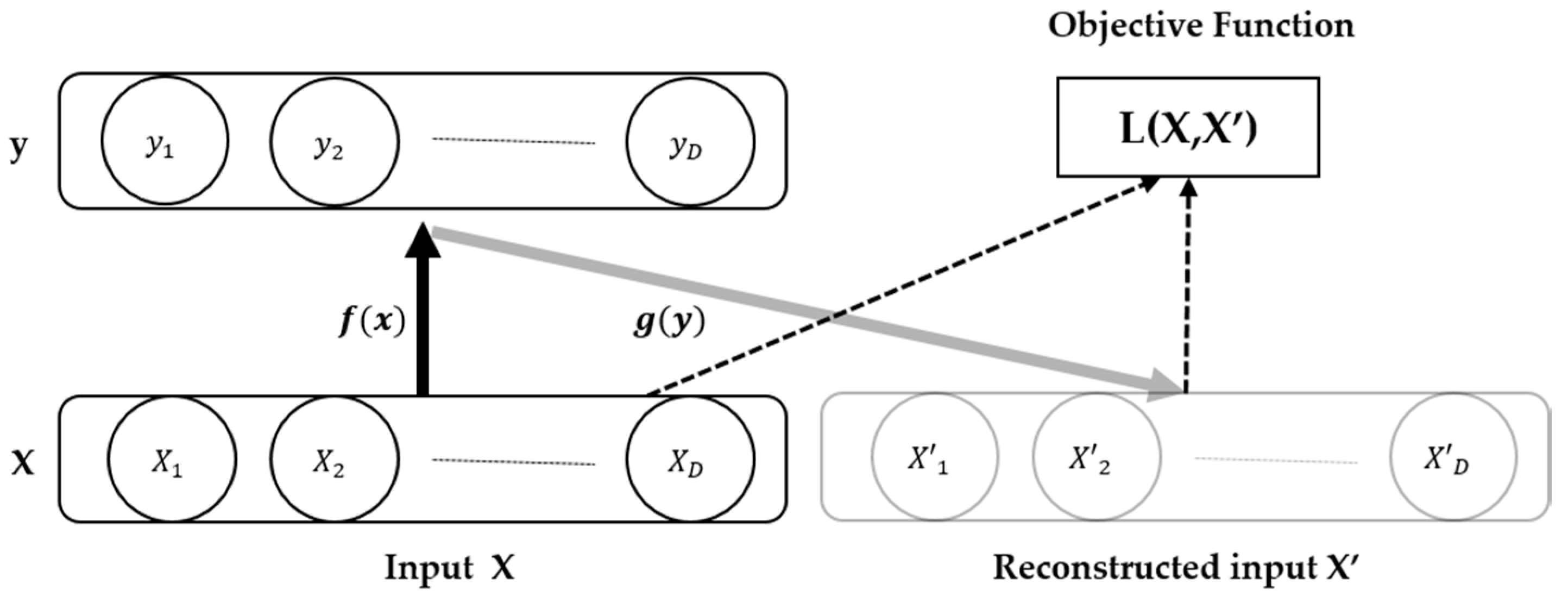
2.1. Auto-Encoder
| Pseudocode of Auto-Encoder |
Procedure Auto-Encoder
Go to Step.3 Finish training |
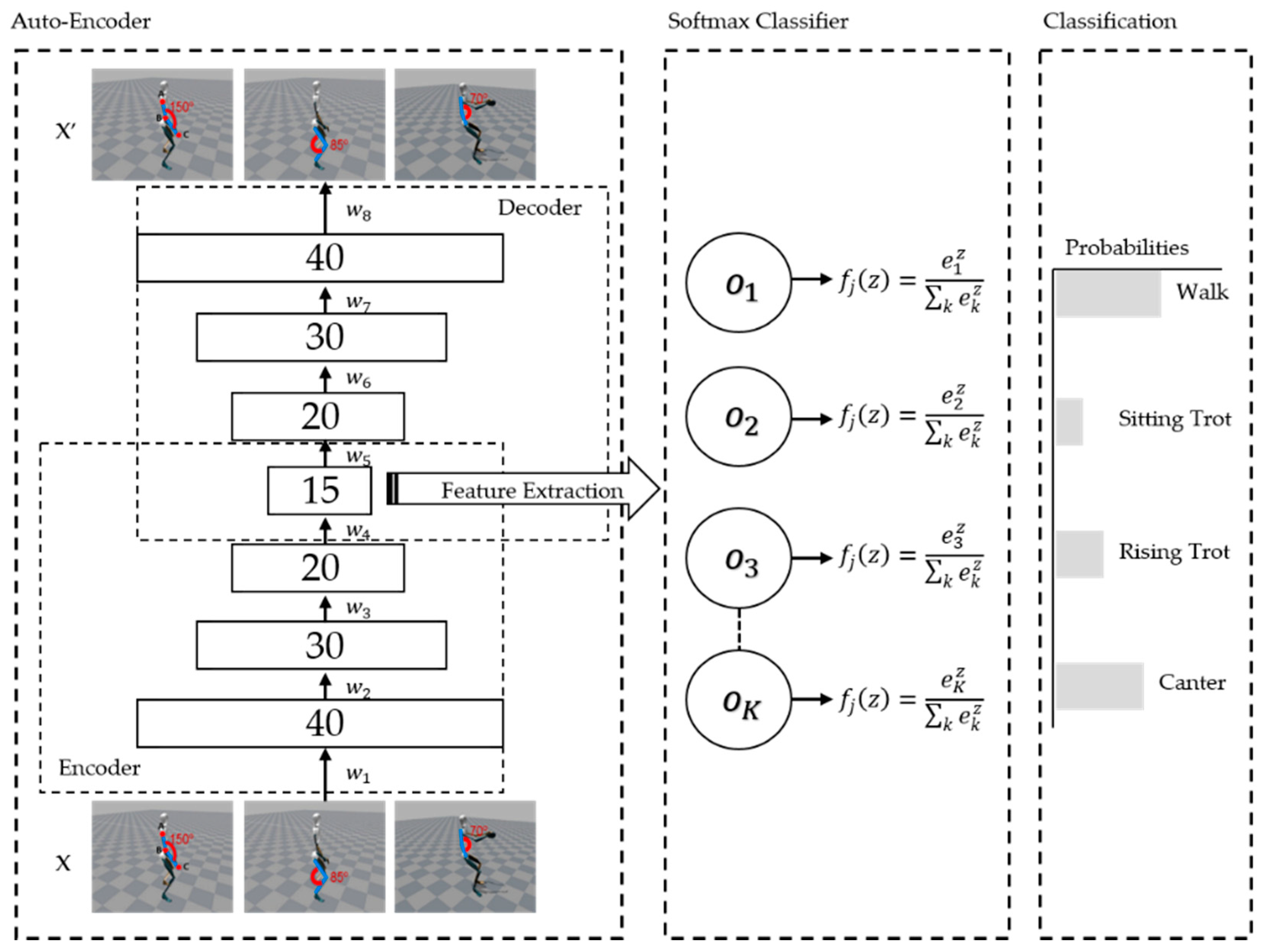
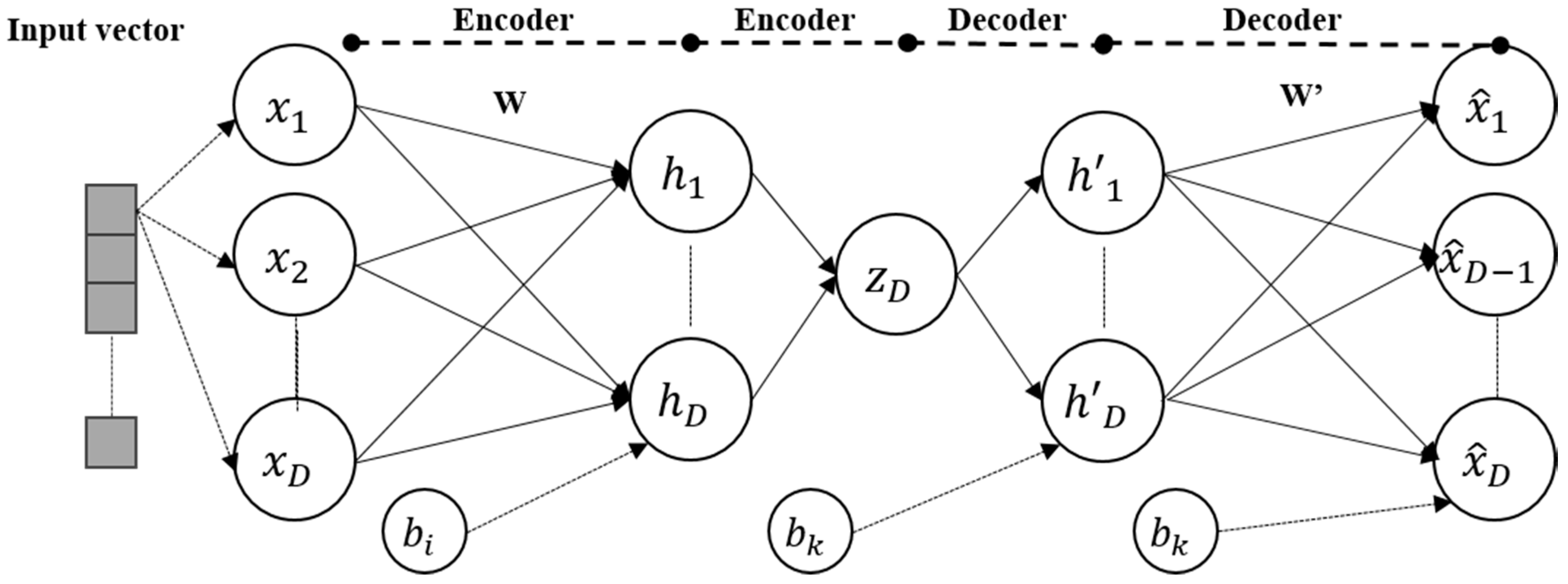
2.2. Stacked Auto-Encoder
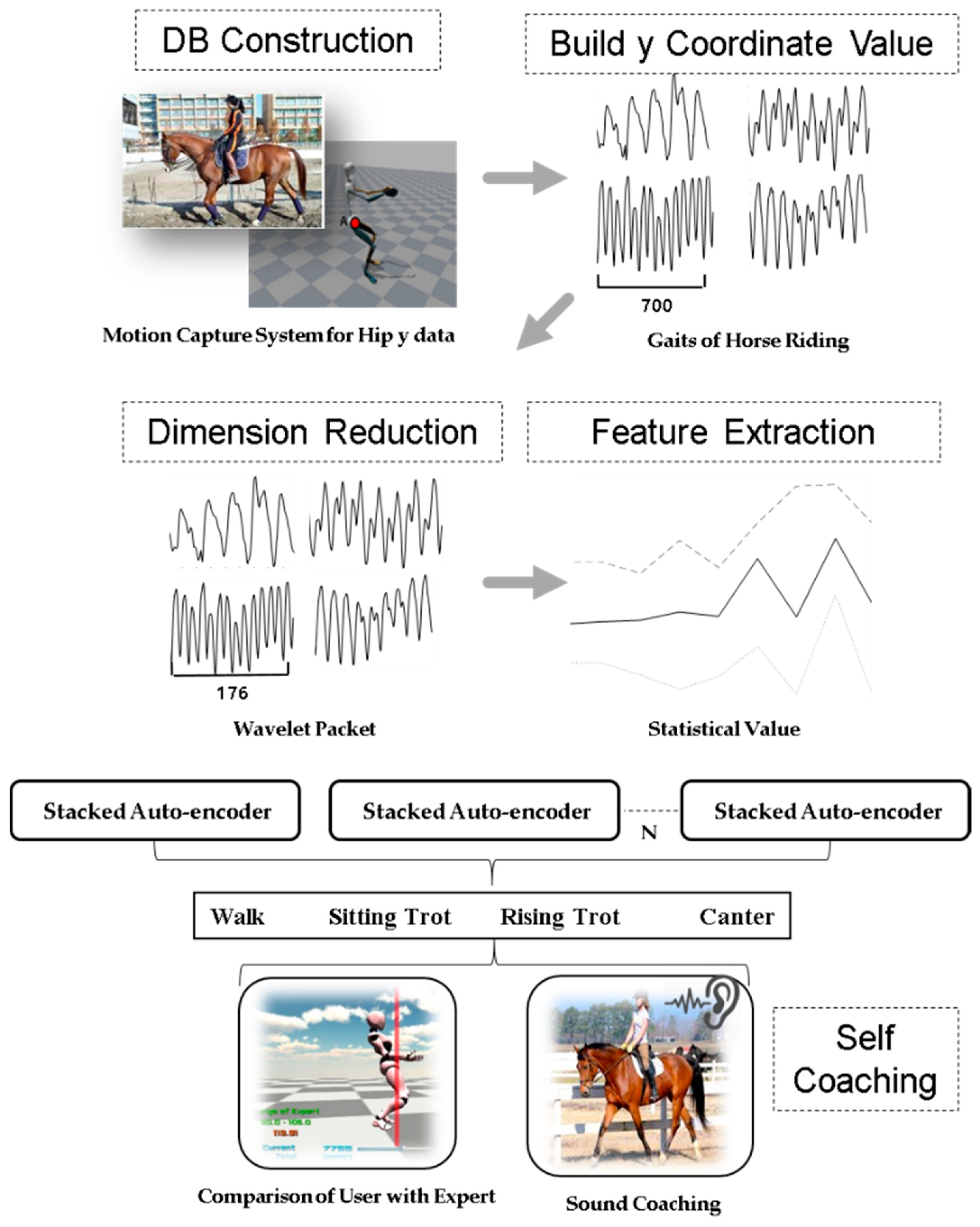
3. Proposed Method
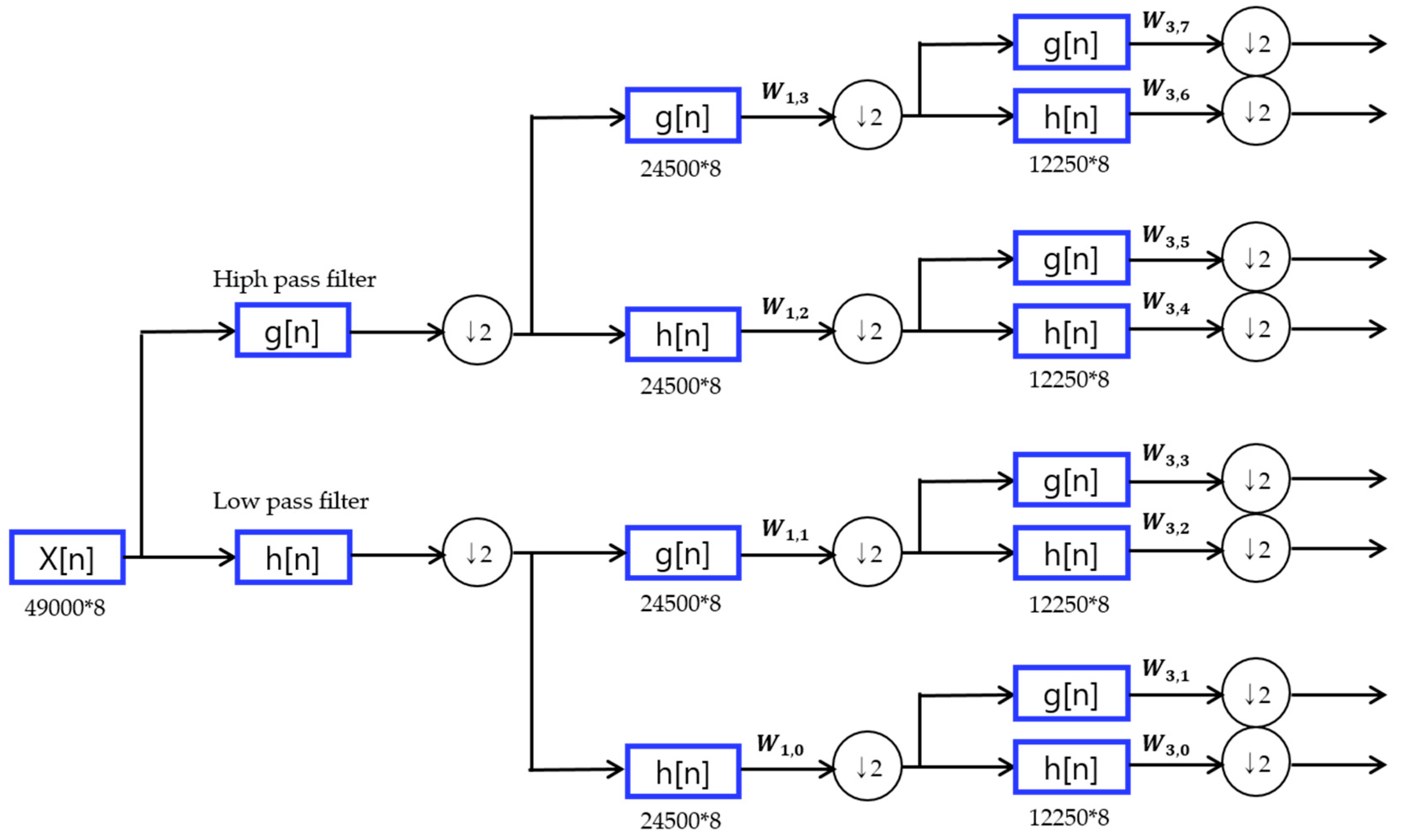
3.1. Compression Method Using Wavelet Packet
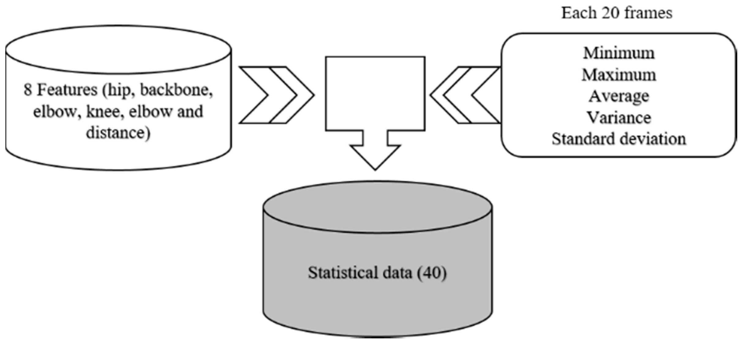
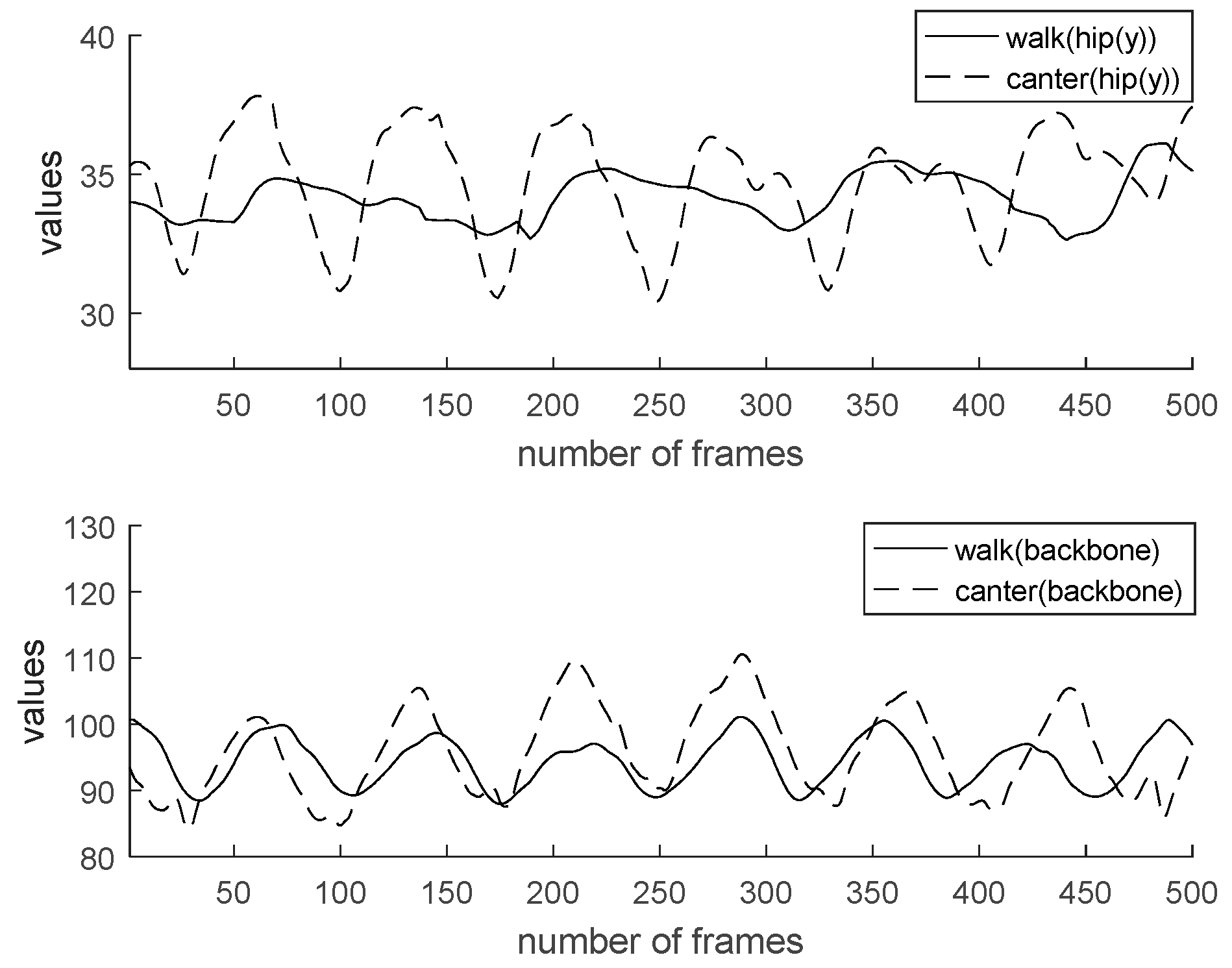
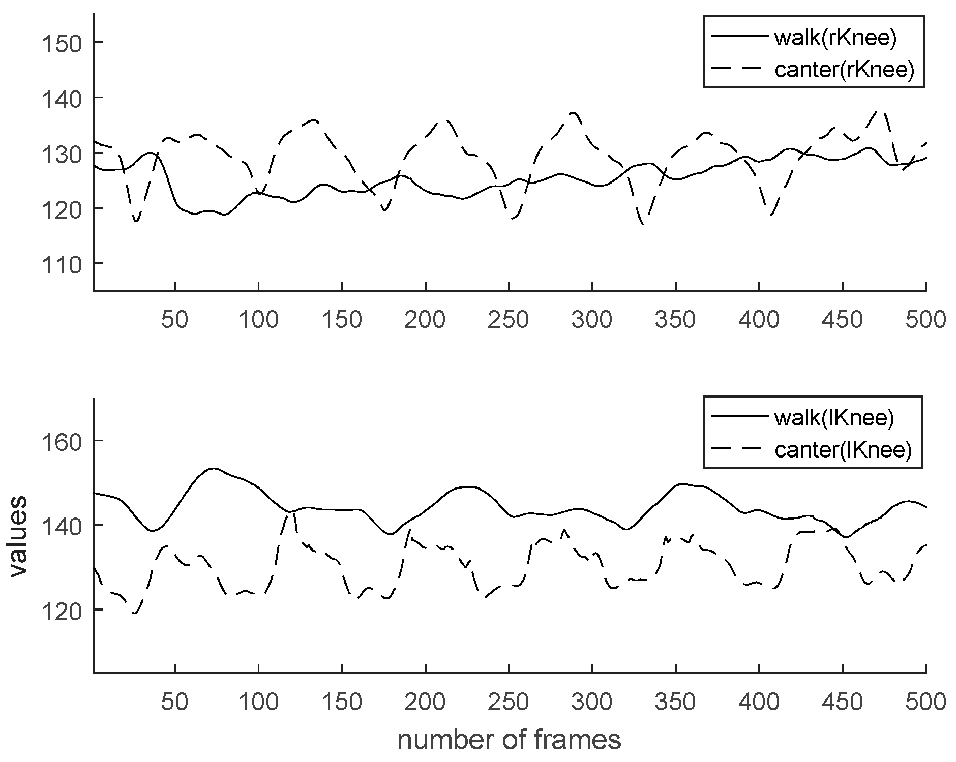
3.2. Feature Extraction Based on Statistical Methods
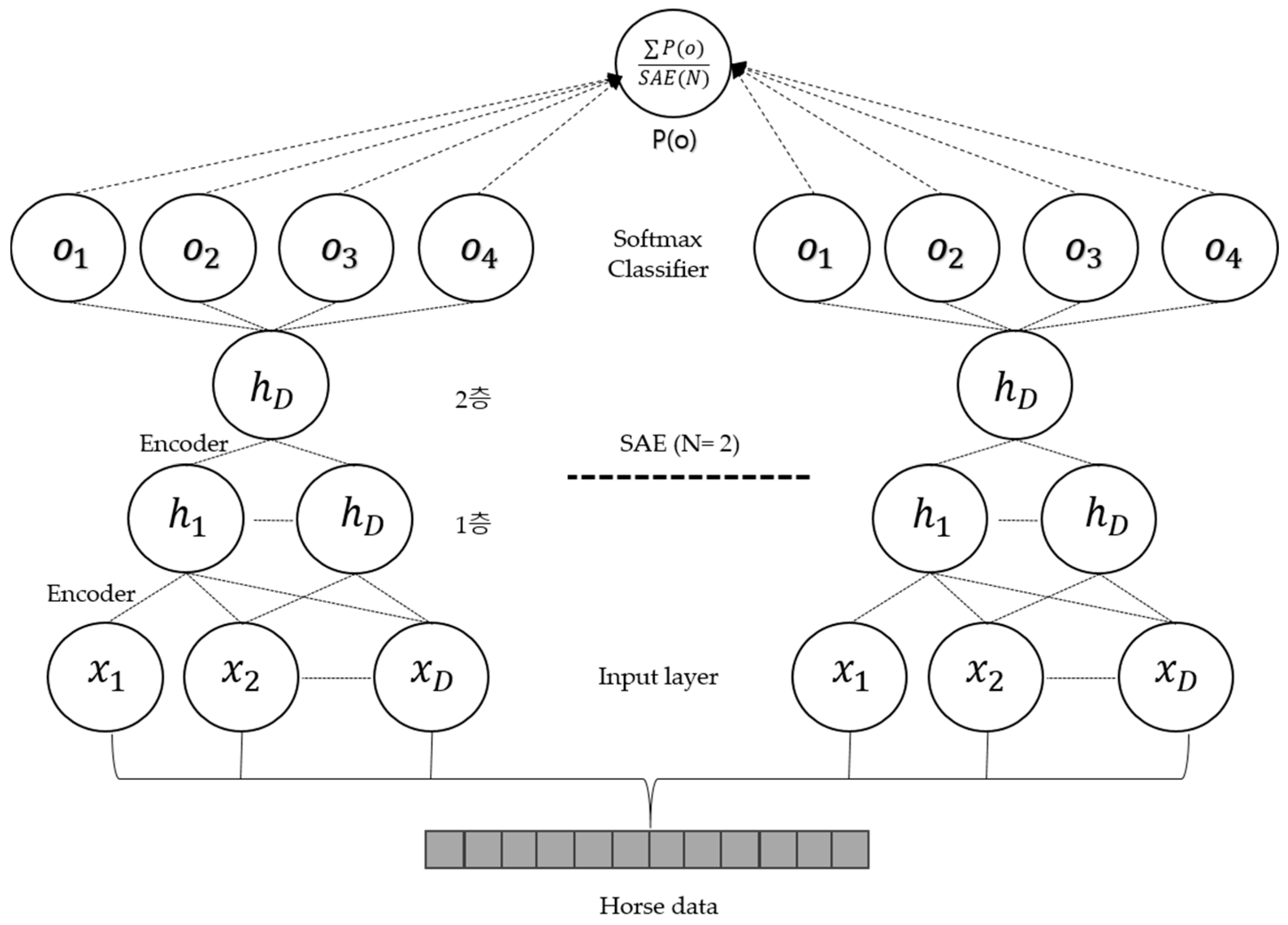
3.3. Ensemble Stacked Auto-Encoder
| Pseudocode of Stacked Auto-Encoder |
Procedure Ensemble Stacked Auto-Encoder
Go to Step.3 Finish training |
4. Experiment and Database
4.1. Sensors of MVN Based Upon Miniature MEMS Inertial Sensor Technology
4.2. Database
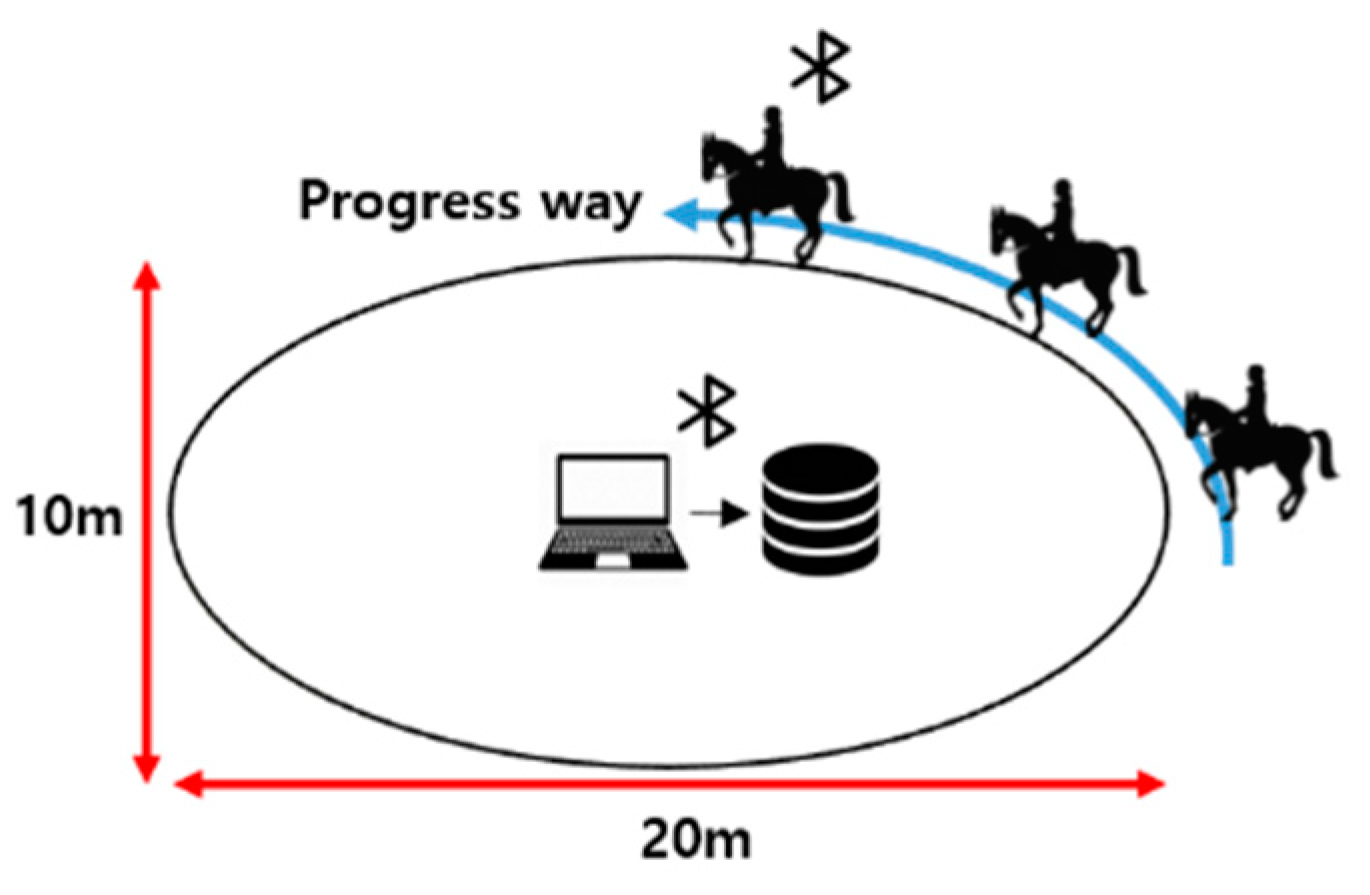
4.3. Environment
4.4. Coaching for Horse Riding
4.5. Experiment and Result
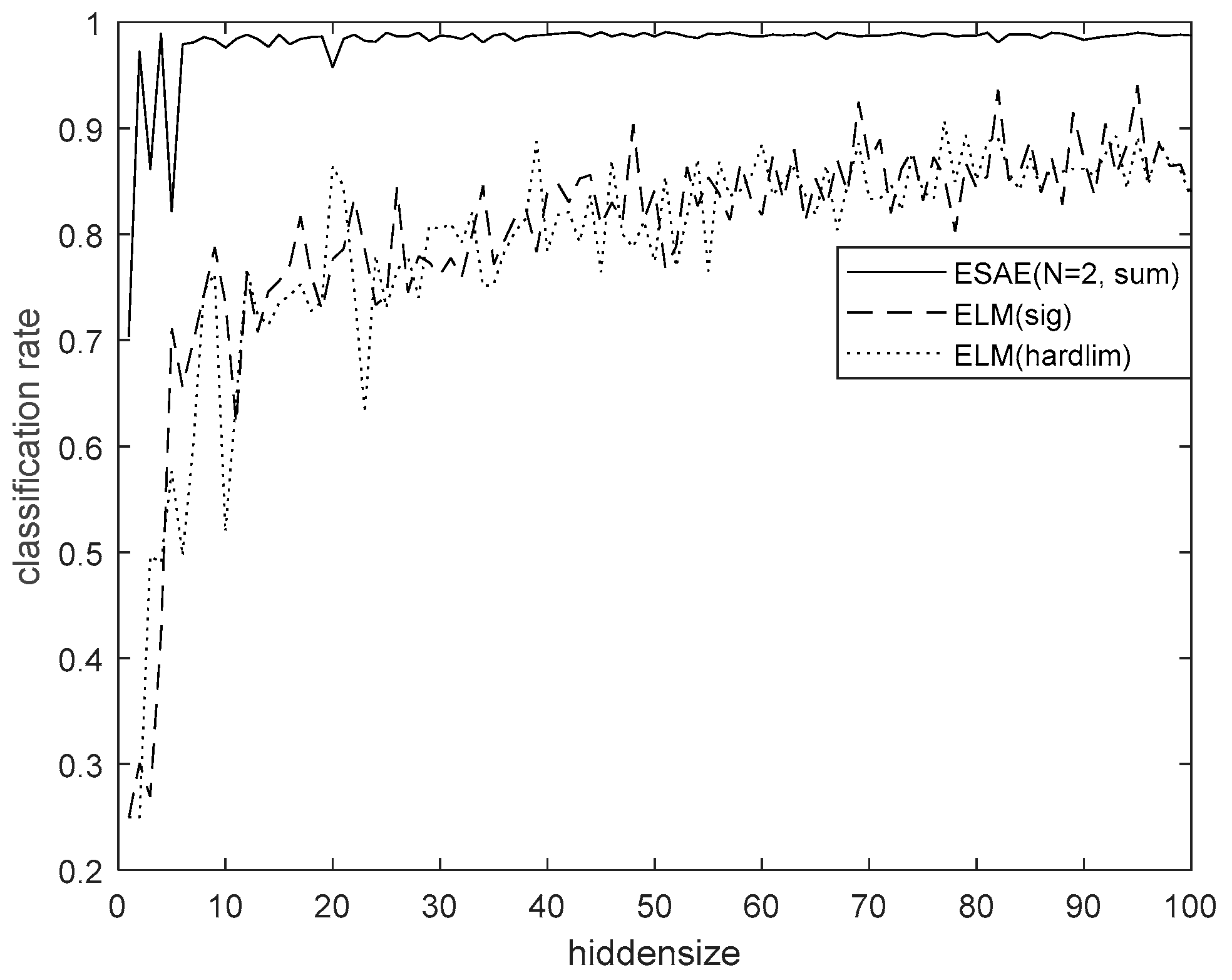
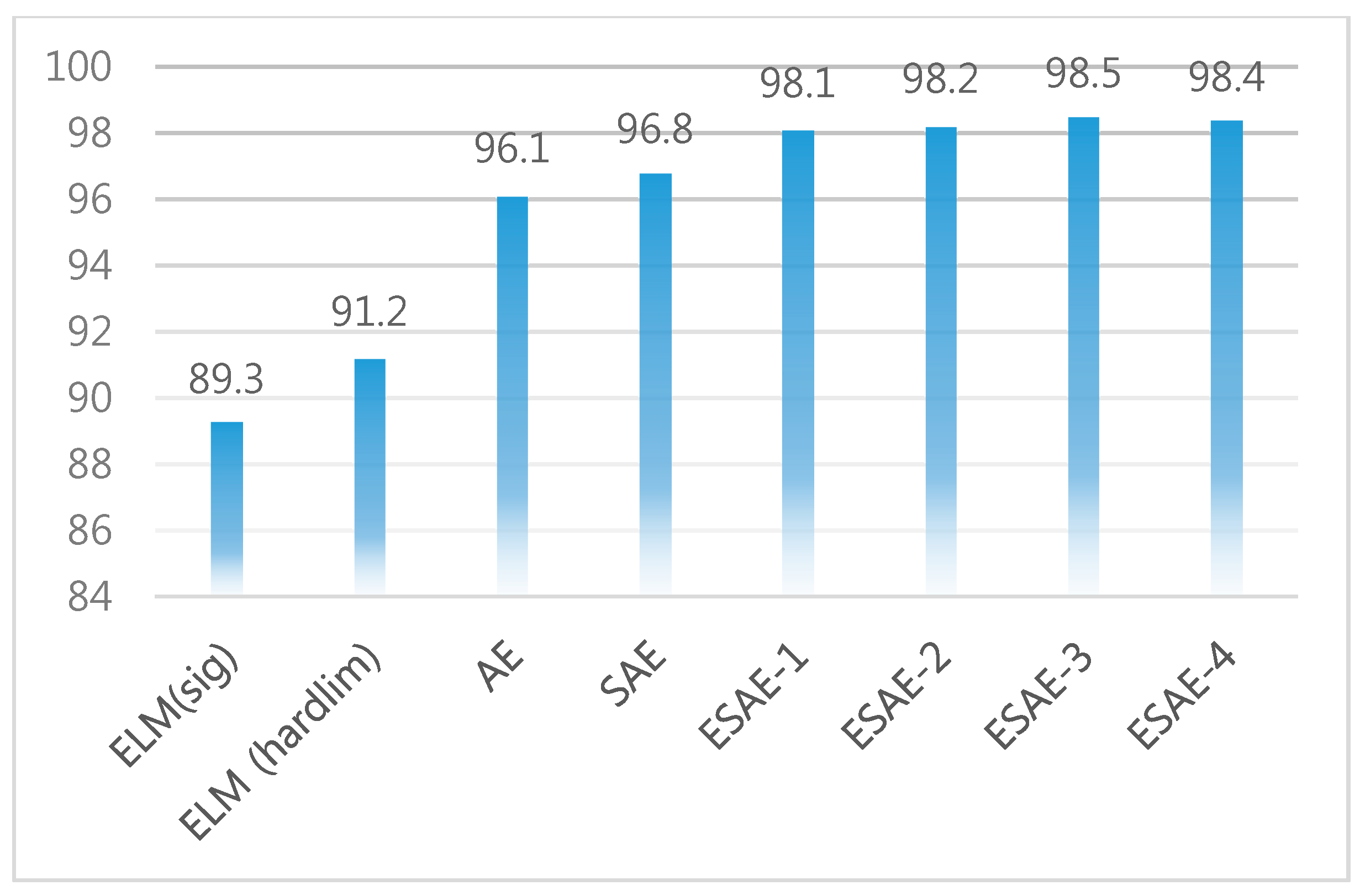
4.6. Classification Performance
5. Conclusions
Author Contributions
Funding
Conflicts of Interest
References
- Manic, M.; Rieger, C. Intelligent buildings of the future: Cyberaware, deep learning powered and human interacting. Ind. Electron. Mag. 2016, 10, 32–49. [Google Scholar] [CrossRef]
- Deng, W.; Hu, J.; Guo, J. Transform-invariant PCA: A unified approach to fully automatic face alignment, representation, and recognition. IEEE Trans. Pattern Anal. Mach. Intell. 2014, 36, 1275–1284. [Google Scholar] [CrossRef] [PubMed]
- Fourati, H.; Manamanni, N.; Afilal, L.; Handrich, Y. Complementary Observer for Body Segments Motion Capturing by Inertial and Magnetic Sensors. IEEE/ASME Trans. Mechatron. 2014, 19, 149–157. [Google Scholar] [CrossRef]
- Fourati, H. Heterogeneous data fusion algorithm for pedestrian navigation via foot-mounted inertial measurement unit and complementary filter. IEEE Trans. Instrum. Meas. 2015, 64, 221–229. [Google Scholar] [CrossRef]
- Zihajehzadeh, S.; Yoon, P.K.; Kang, B.S.; Park, E.J. UWB-Aided inertial motion capture for lower body 3-D dynamic activity and trajectory tracking. IEEE Trans. Instrum. Meas. 2015, 64, 3577–3587. [Google Scholar] [CrossRef]
- Vartiainen, P.; Bragge, T.; Arokoski, J.P.; Karjalainen, P.A. Nonlinear state-space modeling of human motion using 2-D marker observations. IEEE Trans. Biomed. Eng. 2014, 61, 2167–2178. [Google Scholar] [CrossRef] [PubMed]
- Wang, Y.; Hoai, M. Improving human action recognition by non-action classification. In Proceedings of the 2016 IEEE Conference on Computer Vision and Pattern Recognition (CVPR), Las Vegas, NV, USA, 27–30 June 2016; pp. 2698–2707. [Google Scholar]
- Ligorio, G.; Sabatini, A.M. A novel kalman filter for human motion tracking with an inertial-based dynamic inclinometer. IEEE Trans. Biomed. Eng. 2015, 62, 2033–2043. [Google Scholar] [CrossRef] [PubMed]
- Yilmaz, A.; Orhanli, T. Gait motion simulator for kinematic tests of above knee prostheses. IET Sci. Meas. Technol. 2015, 9, 250–258. [Google Scholar] [CrossRef]
- Zhang, Y.; Chen, K.; Yi, J.; Liu, T.; Pan, Q. Whole-body pose estimation in human bicycle riding using a small set of wearable sensors. IEEE/ASME Trans. Mechatron. 2016, 21, 163–174. [Google Scholar] [CrossRef]
- Villeneuve, E.; Harwin, W.; Holderbaum, W.; Sherratt, R.S. Signal quality and compactness of a dual-accelerometer system for gyro-free human motion analysis. IEEE Sens. J. 2016, 16, 6261–6269. [Google Scholar] [CrossRef]
- Sarafianos, N.; Boteanu, B.; Ionescu, B.; Kakadiaris, A. 3D Human pose estimation: A review of the literature and analysis of covariates. Comput. Vis. Image Underst. 2016, 152, 1–20. [Google Scholar] [CrossRef]
- Hasan, M.; Chowdhury, K.R. A continuous learning framework for activity recognition using deep hybrid feature models. IEEE Trans. Multimedia 2015, 17, 1909–1922. [Google Scholar] [CrossRef]
- Hong, C.; Yu, J. Multimodal deep autoencoder for human pose recovery. IEEE Trans. Image Process. 2015, 24, 5659–5670. [Google Scholar] [CrossRef] [PubMed]
- Liu, H.; Taniguchi, T. Feature extraction and pattern recognition for human motion by a deep sparse autoencoder. In Proceedings of the 2014 IEEE International Conference on Computer and Information Technology, Xi’an, China, 11–13 September 2014; pp. 174–181. [Google Scholar]
- Yin, X.; Chen, Q. Deep metric learning autoencoder for nonlinear temporal alignment of human motion. In Proceedings of the 2016 IEEE International Conference on Robotics and Automation (ICRA), Stockholm, Sweden, 16–21 May 2016; pp. 2160–2166. [Google Scholar]
- Hossein, R.; Ajmal, M.; Mubarak, S. Learning a deep model for human action recognition from novel viewpoints. IEEE Trans. PAMI 2018, 40, 667–681. [Google Scholar]
- Potapov, A.; Potapova, V.; Peterson, M. A feasibility study of an autoencoder meta-model for improving generalization capabilities on training sets of small sizes. Pattern Recognit. Lett. 2016, 80, 24–29. [Google Scholar] [CrossRef]
- Xu, C.; Liu, Q.; Ye, M. Age invariant face recognition and retrieval by coupled auto-encoder networks. Neurocomputing 2017, 222, 62–71. [Google Scholar] [CrossRef]
- Kamyshanska, H.; Memisevic, R. The potential energy of an autoencoder. IEEE Trans. Pattern Anal. Mach. Intell. 2015, 37, 1261–1273. [Google Scholar] [CrossRef] [PubMed]
- Geng, J.; Wang, H. Deep supervised and contractive neural network for SAR image classification. IEEE Geosci. Remote Sens. 2017, 55, 2442–2459. [Google Scholar] [CrossRef]
- Zeng, K.; Yu, J. Coupled deep autoencoder for single image super-resolution. IEEE Trans. Cybern. 2017, 47, 27–37. [Google Scholar] [CrossRef] [PubMed]
- Shi, B.; Chen, Y.; Zhang, P.; Smith, C.D. Nonlinear feature transformation and deep fusion for Alzheimer’s disease staging analysis. Pattern Recognit. 2017, 63, 487–498. [Google Scholar] [CrossRef]
- Saponara, S. Wearable biometric performance measurement system for combat sports. IEEE Trans. Instrum. Meas. 2017, 66, 2545–2555. [Google Scholar] [CrossRef]
- Seshadri, D.R.; Drummond, C.; Craker, J.; Rowbottom, J.R. Wearable devices for sports: New integrated technologies allow coaches, physicians, and trainers to better understand the physical demands of athletes in real time. IEEE Pulse 2017, 8, 38–43. [Google Scholar] [CrossRef] [PubMed]
- Lee, J.N.; Lee, M.W.; Byeon, Y.H.; Lee, W.S.; Kwak, K.C. Classification of horse gaits using FCM-based neuro-fuzzy classifier from the transformed data information of inertial sensor. Sensors 2016, 16. [Google Scholar] [CrossRef] [PubMed]


| Symbol | Definition | Symbol | Definition |
|---|---|---|---|
| Size of input layer (= output) | Size of hidden layer | ||
| The j-th weight of the i-th output layer neuron | The output value of the j-th hidden layer neuron for the n-th learning vector | ||
| Learning rate | The output value of the i-th output layer neuron for the n-th learning vector | ||
| The i-th element of the n-th learning vector | Bias of the j-th hidden layer neuron | ||
| The j-th weight of the j-th hidden layer neuron | Bias of i-th output layer neuron |
| Feature | Minimum of Rising Trot | Maximum of Rising Trot | Minimum of Canter | Maximum of Canter |
|---|---|---|---|---|
| Hip y | 32.08 | 38.79 | 31.87 | 38.31 |
| Backbone | 171.39 | 176.47 | 170.77 | 176.34 |
| Angle of elbow | 127.59 | 151.82 | 124.98 | 159.24 |
| Angle of knee | 123.92 | 172.20 | 119.50 | 135.80 |
| Distance of elbow | 23.02 | 27.02 | 25.87 | 25.78 |
| Distance of knee | 14.93 | 16.42 | 15.52 | 18.59 |
| Method | Performance |
|---|---|
| LDA | 87.0 |
| SVM | 94.5 |
| TREE | 84.1 |
| KNN | 94.0 |
| Ensemble Bagging | 91.3 |
| ELM (Sin) | 91.8 |
| ELM (Sig) | 91.1 |
| AE (Hidden Size = 15) | 94.1 |
| SAE (Hidden Size = 10, 15) | 94.2 |
| ESAE-1 (n = 3, sum) | 94.2 |
| ESAE-2 (n = 3, product) | 94.3 |
| ESAE-3 (n = 2, sum) | 95.3 |
| ESAE-4 (n = 2, product) | 95.2 |
© 2018 by the authors. Licensee MDPI, Basel, Switzerland. This article is an open access article distributed under the terms and conditions of the Creative Commons Attribution (CC BY) license (http://creativecommons.org/licenses/by/4.0/).
Share and Cite
Lee, J.-N.; Byeon, Y.-H.; Kwak, K.-C. Design of Ensemble Stacked Auto-Encoder for Classification of Horse Gaits with MEMS Inertial Sensor Technology. Micromachines 2018, 9, 411. https://doi.org/10.3390/mi9080411
Lee J-N, Byeon Y-H, Kwak K-C. Design of Ensemble Stacked Auto-Encoder for Classification of Horse Gaits with MEMS Inertial Sensor Technology. Micromachines. 2018; 9(8):411. https://doi.org/10.3390/mi9080411
Chicago/Turabian StyleLee, Jae-Neung, Yeong-Hyeon Byeon, and Keun-Chang Kwak. 2018. "Design of Ensemble Stacked Auto-Encoder for Classification of Horse Gaits with MEMS Inertial Sensor Technology" Micromachines 9, no. 8: 411. https://doi.org/10.3390/mi9080411
APA StyleLee, J.-N., Byeon, Y.-H., & Kwak, K.-C. (2018). Design of Ensemble Stacked Auto-Encoder for Classification of Horse Gaits with MEMS Inertial Sensor Technology. Micromachines, 9(8), 411. https://doi.org/10.3390/mi9080411