
Design and Analysis of MEMS Linear Phased Array

Abstract
: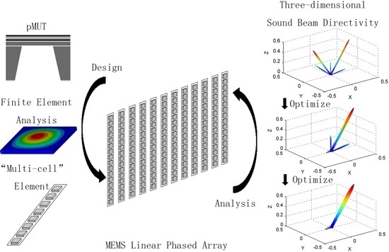
1. Introduction
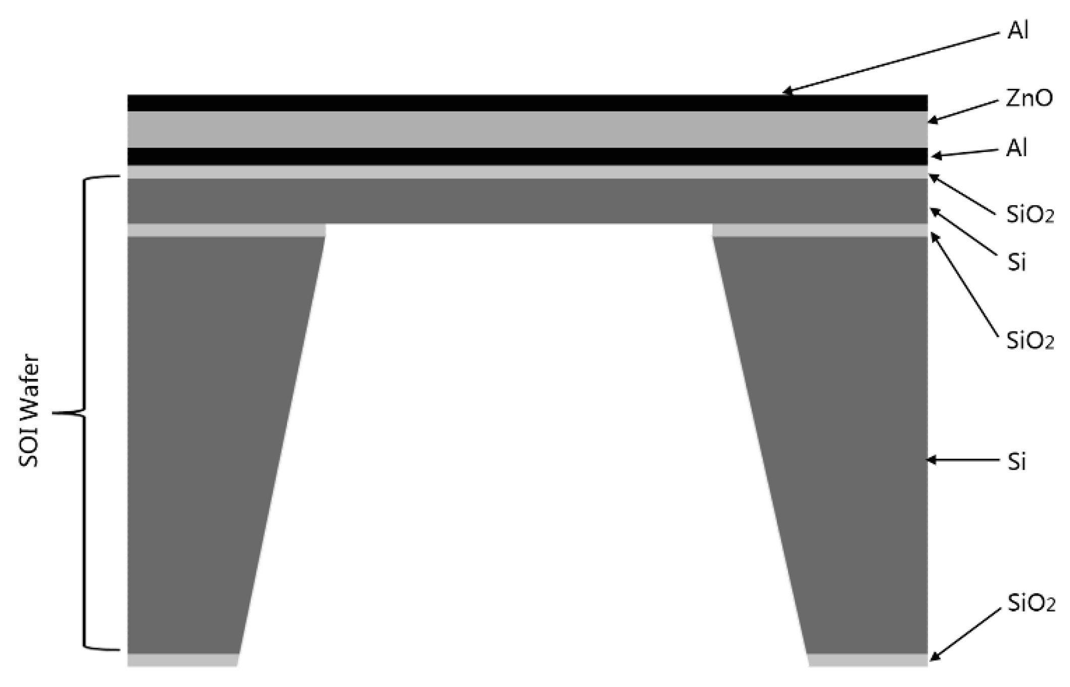
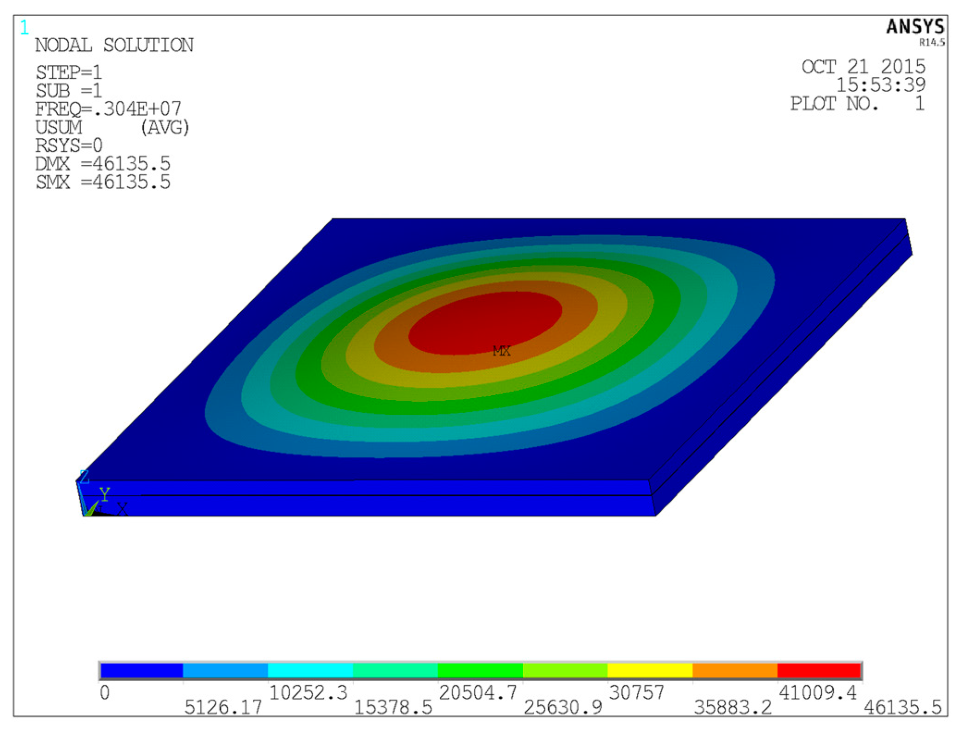
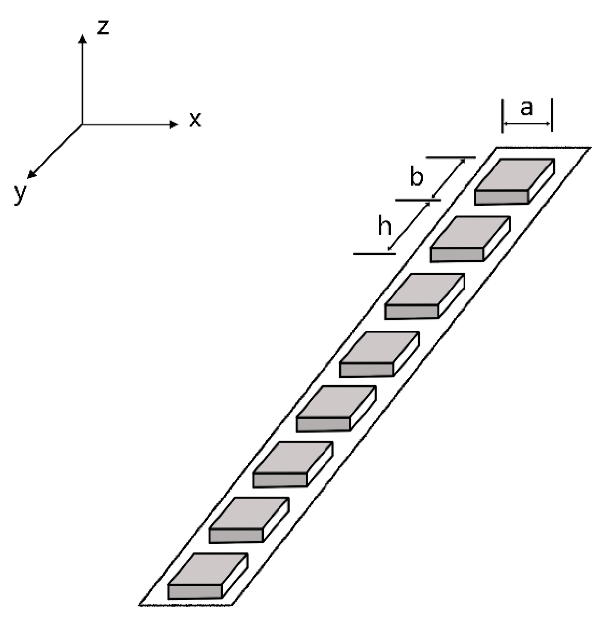
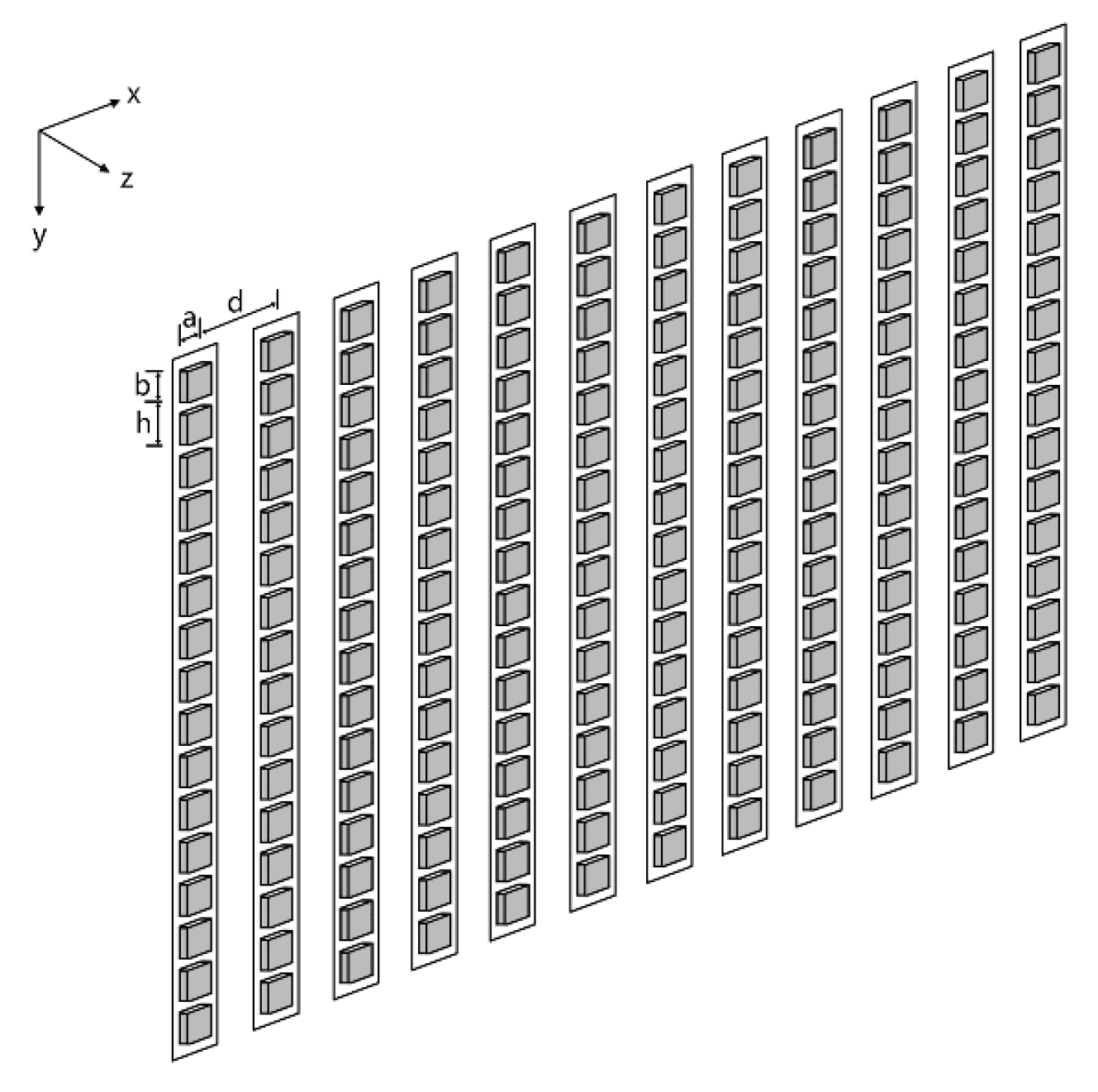
2. MEMS Linear Phased Array Element Structure

| Thickness of Si | Thickness of SiO2 | Thickness of ZnO | Length of Membrane |
|---|---|---|---|
| 8 μm | 0.2 μm | 6 μm | 228 μm |
| Material | Young’s Modulus (GPa) | Density (103 kg/m3) | Poisson Ratio |
|---|---|---|---|
| Si | 167 | 2.33 | 0.28 |
| SiO2 | 72 | 2.30 | 0.16 |
| ZnO | 120 | 5.68 | 0.446 |

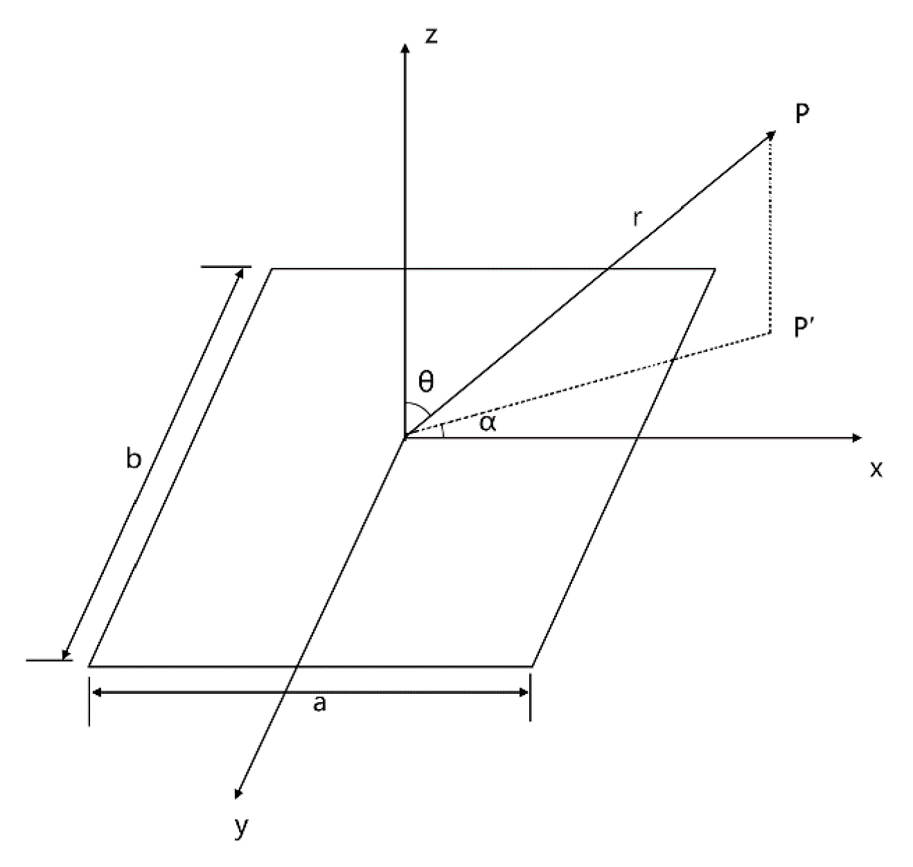
3. MEMS Linear Phased Array Beam Directivity
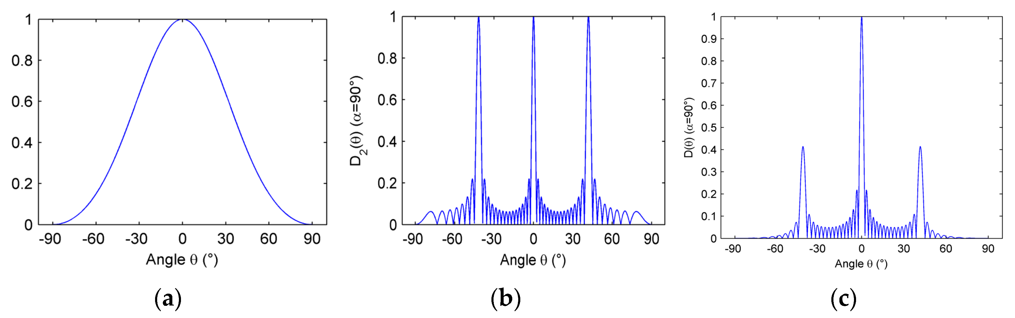
- The directivity of a single element

- 2.
- The uniform linear array directivity
4. Optimization and Simulation
4.1. Optimization in the Elevation Direction (y-z Plane, α = α0 = 90°)
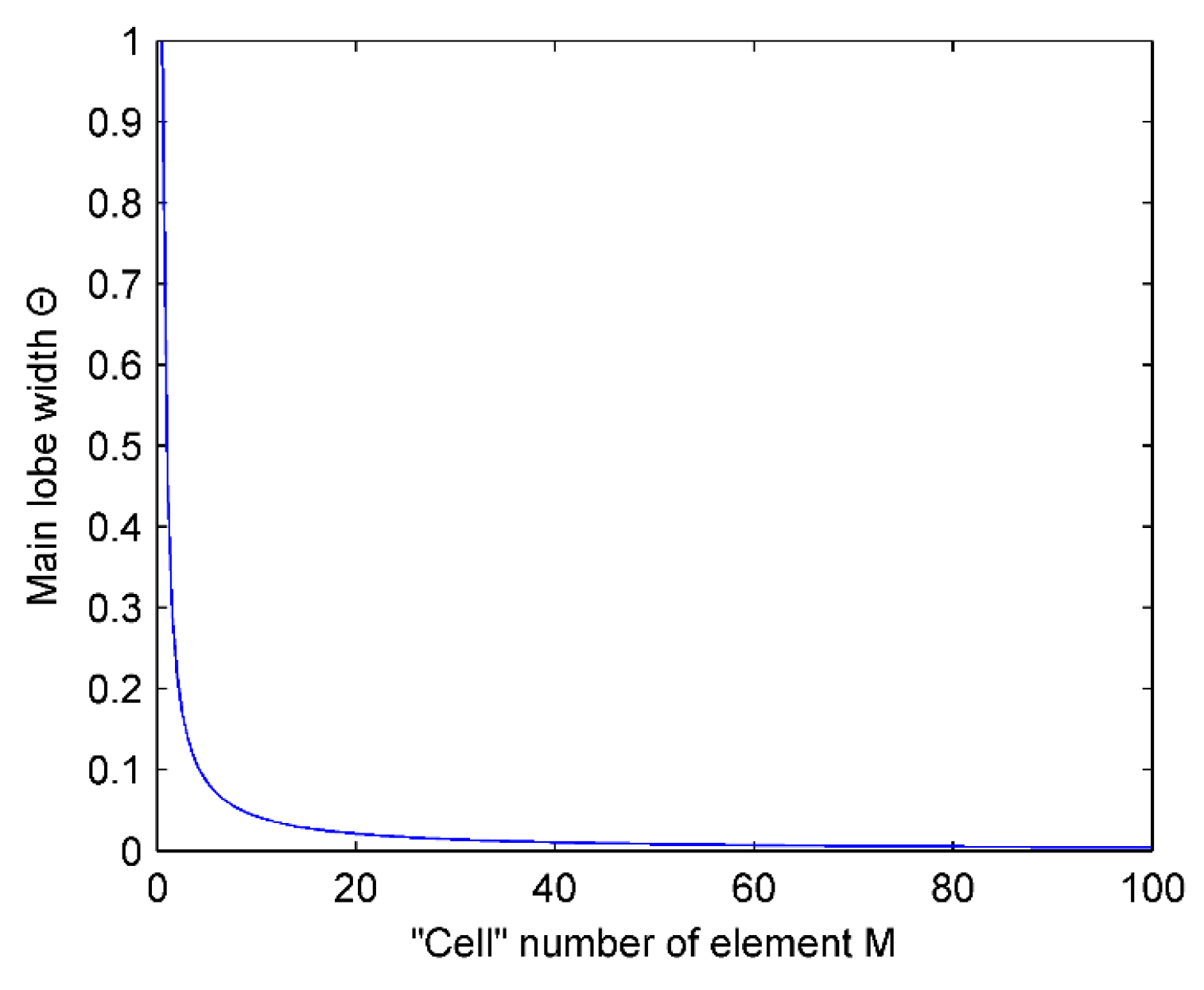
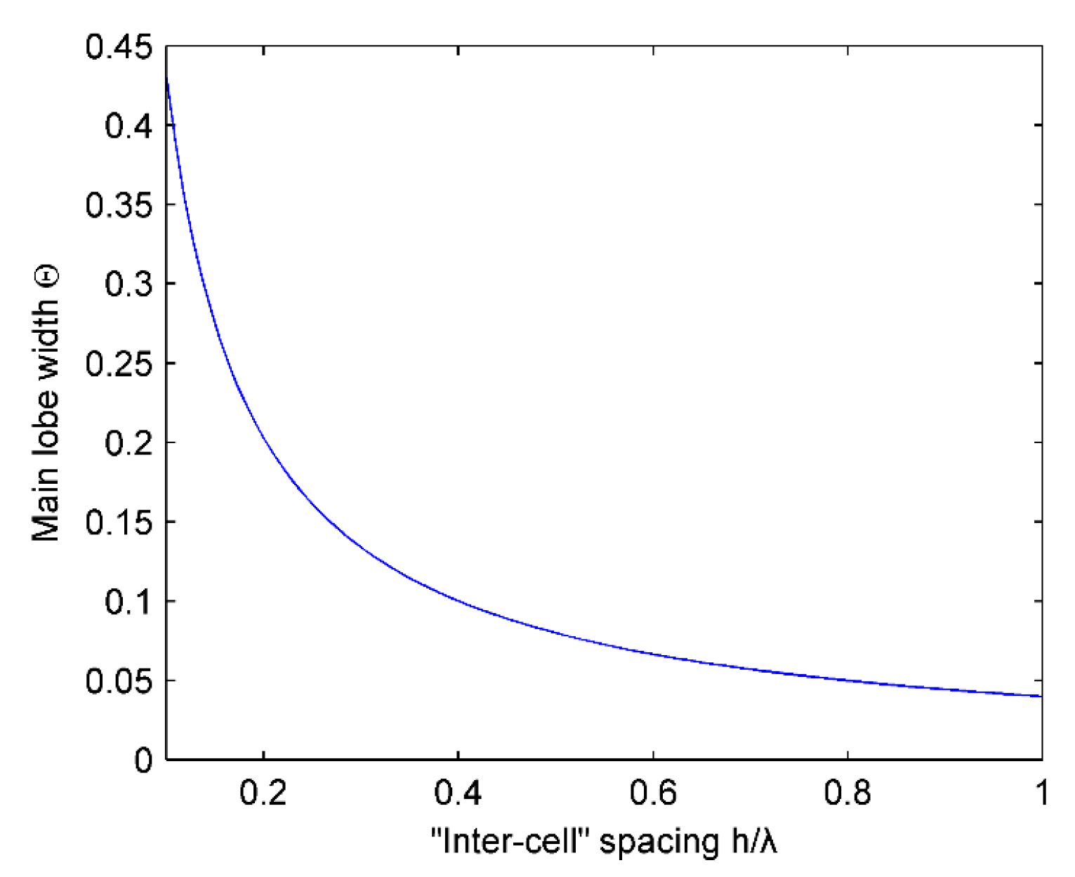
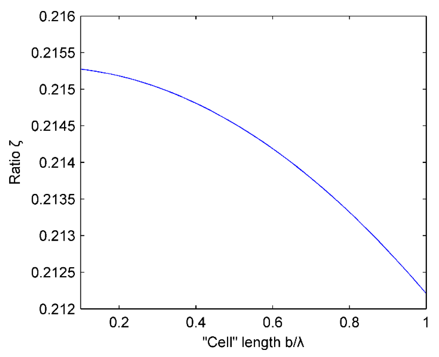
4.1.1. Main Lobe
4.1.2. Grating Lobe and Side Lobe


4.2. Optimization in the Lateral Direction (x-z Plane, α = α0 = 0°)
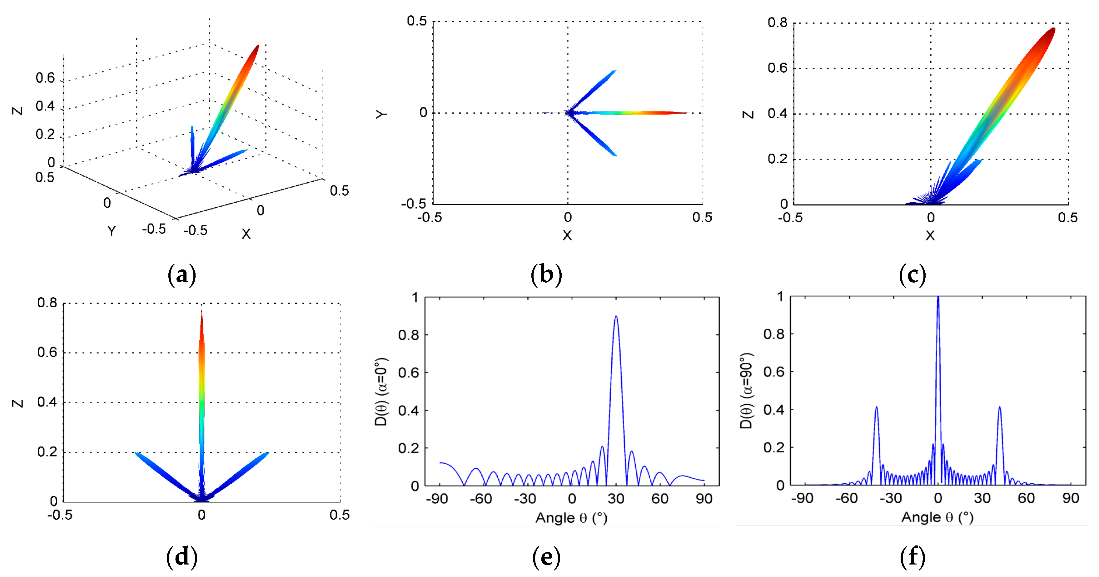
4.3. Simulation Results


5. Conclusions
Acknowledgments
Author Contributions
Conflicts of Interest
References
- Akasheh, F.; Fraser, J.D.; Bose, S.; Bandyopadhyay, A. Piezoelectric micromachined ultrasonic transducers: Modeling the influence of structural parameters on device performance. IEEE Trans. Ultrason. Ferroelectr. Freq. Control 2005, 52, 455–468. [Google Scholar] [CrossRef] [PubMed]
- Hedegaard, T.; Pedersen, T.; Thomsen, E.V.; Lou-Møller, R.; Hansen, K.; Zawada, T. Screen printed thick film based pMUT arrays. In Proceedings of the IEEE Ultrasonics Symposium, Beijing, China, 2–5 November 2008; pp. 2126–2129.
- Dausch, D.E.; Gilchrist, K.H.; Carlson, J.R.; Castellucci, J.B.; Chou, D.R.; Von Ramm, O.T. Improved pulse-echo imaging performance for flexure-mode pMUT arrays. In Proceedings of the IEEE Ultrasonics Symposium (IUS), San Diego, CA, USA, 11–14 October 2010; pp. 451–454.
- Pedersen, T.; Zawada, T.; Hansen, K.; Lou-Møller, R.; Thomsen, E.V. Fabrication of high-frequency pMUT arrays on silicon substrates. IEEE Trans. Ultrason. Ferroelectr. Freq. Control 2010, 57, 1470–1477. [Google Scholar] [CrossRef] [PubMed]
- Lu, Y.; Tang, H.Y.; Fung, S.; Boser, B.E.; Horsley, D. Short-range and high-resolution ultrasound imaging using an 8 MHz Aluminum Nitride PMUT array. In Proceedings of the 28th IEEE International Conference on Micro Electro Mechanical Systems (MEMS), Estoril, Portugal, 18–22 January 2015; pp. 140–143.
- Griggio, F.; Demore, C.E.; Kim, H.; Gigliotti, J.; Qiu, Y.; Jackson, T.N.; Choi, K.; Tutwiler, R.L.; Cochran, S.; Trolier-Mckinstry, S. Micromachined diaphragm transducers for miniaturised ultrasound arrays. In Proceedings of the IEEE International Ultrasonics Symposium (IUS), Dresden, Germany, 7–10 October 2012; pp. 1–4.
- Lu, Y.; Horsley, D. Modeling, fabrication, and characterization of piezoelectric micromachined ultrasonic transducer arrays based on cavity SOI wafers. J. Microelectromech. Syst. 2015, 24, 1142–1149. [Google Scholar] [CrossRef]
- Iguchi, S. Die Biegungsschwingungen der vierseitig eingespannten rechteckigen Platte. Arch. Appl. Mech. 1937, 8, 11–25. [Google Scholar] [CrossRef]
- Yamashita, K.; Katata, H.; Okuyama, M.; Miyoshi, H.; Kato, G.; Aoyagi, S.; Suzuki, Y. Arrayed ultrasonic microsensors with high directivity for in-air use using PZT thin film on silicon diaphragms. Sens. Actuators A Phys. 2002, 97–98, 302–307. [Google Scholar] [CrossRef]
- Dausch, D.E.; Castellucci, J.B.; Chou, D.R.; Von Ramm, O.T. Theory and operation of 2-D array piezoelectric micromachined ultrasound transducers. IEEE Trans. Ultrason. Ferroelectr. Freq. Control 2008, 55, 2484–2492. [Google Scholar] [CrossRef] [PubMed]
- Steinberg, B.D. Principles of Aperture and Array System Design: Including Random and Adaptive Arrays; John Wiley & Sons: New York, NY, USA, 1976. [Google Scholar]
- Lemon, D.K.; Posakony, G.J. Linear array technology in NDE applications. Mater. Eval. 1980, 38, 34–37. [Google Scholar]
- Turnbull, D.H.; Foster, F.S. Beam steering with pulsed two-dimensional transducer arrays. IEEE Trans. Ultrason. Ferroelectr. Freq. Control 1991, 38, 320–333. [Google Scholar] [CrossRef] [PubMed]
- Wooh, S.C.; Shi, Y. Influence of phased array element size on beam steering behavior. Uhrasonis 1998, 36, 737–749. [Google Scholar] [CrossRef]
- Wooh, S.C.; Shi, Y. Optimum beam steering of linear phased arrays. Wave Motion 1999, 29, 245–265. [Google Scholar] [CrossRef]
- Wooh, S.C.; Shi, Y. A simulation study of the beam steering characteristics for linear phased arrays. J. Nondestr. Eval. 1999, 18, 39–57. [Google Scholar] [CrossRef]
- Clay, A.C.; Wooh, S.C.; Azar, L.; Wang, J.Y. Experimental study of phased array beam steering characteristics. J. Nondestr. Eval. 1999, 18, 59–71. [Google Scholar] [CrossRef]
- Wooh, S.C.; Shi, Y. Three-dimensional beam directivity of phase-steered ultrasound. J. Acoust. Soc. Am. 1999, 105, 3275–3282. [Google Scholar] [CrossRef]
© 2016 by the authors; licensee MDPI, Basel, Switzerland. This article is an open access article distributed under the terms and conditions of the Creative Commons by Attribution (CC-BY) license ( http://creativecommons.org/licenses/by/4.0/).
Share and Cite
Fan, G.; Li, J.; Wang, C. Design and Analysis of MEMS Linear Phased Array. Micromachines 2016, 7, 8. https://doi.org/10.3390/mi7010008
Fan G, Li J, Wang C. Design and Analysis of MEMS Linear Phased Array. Micromachines. 2016; 7(1):8. https://doi.org/10.3390/mi7010008
Chicago/Turabian StyleFan, Guoxiang, Junhong Li, and Chenghao Wang. 2016. "Design and Analysis of MEMS Linear Phased Array" Micromachines 7, no. 1: 8. https://doi.org/10.3390/mi7010008
APA StyleFan, G., Li, J., & Wang, C. (2016). Design and Analysis of MEMS Linear Phased Array. Micromachines, 7(1), 8. https://doi.org/10.3390/mi7010008