Effects of Baffle Configuration on Mixing in a T-Shaped Micro-Channel

Abstract

A numerical study was performed for a T-shaped microchannel to enhance mixing performance through a baffle configuration. The mixing performance was analyzed in terms of the DOM (degree of mixing) and the pressure load between the two inlets and outlet. Four different baffle configurations were designed and simulated to determine how they affect the mixing performance of a T-shaped microchannel. Among the four baffle configurations, a cyclic configuration of baffles produced the best results. It exhibited the fastest growth in the DOM along the microchannel. The cyclic configuration means that four baffles are attached to four side walls of the channel in a cyclic order. The mixing improvement occurs in two ways. One is in the baffle region, when the cyclic configuration causes the fluid flow to rotate in the cross section, unlike other configurations. The other improvement is observed in the remaining outlet branch after the baffle region. This improvement is due to twisting and elongation of the boundary between two fluids. The baffle size and the interval between two consecutive baffles are shown to be optimized in terms of the DOM for a given condition.

1. Introduction

Mixing improvement is one of the essential design goals in microfluidic systems for microreactors and micro-total analysis systems (μTASs). The mixing of reagents in these systems usually occurs in various types of microchannels. However, the fluid flows in these microchannels are extremely slow and the associated channel dimensions are extremely small. The fluid flows in microfluidic systems usually correspond to very low Reynolds numbers. Therefore, molecular diffusion is a major principle of mixing, and the achievement of rapid mixing is a very important design goal for a microchannel.

Various techniques to improve mixing in microchannels have been devised and reported in the literature [1]. These techniques can be classified into three types: passive, active, and combined, depending on whether or not an external energy source is used. Active techniques use various types of external energy sources. Typical energy sources for active techniques include electric [2], electro-magnetic [3], and ultrasonic vibratory fields [4]. The pulsing of inlet flow to a microchannel [1,5] is another active technique. Most passive techniques have been devised to agitate and/or generate secondary flow by means of channel geometry or wall modifications. Therefore, passive techniques could be less effective than active techniques. Nevertheless, passive techniques are widely used in microfluidic systems as they are simpler to fabricate and easier to integrate into microfluidic systems. Examples of the wall modification technique include recessed grooves in the channel wall [6], herringbone-type walls [7], junction contraction [8], indentations and baffles [9,10], and periodic geometric features [11]. A combined method using both passive and active techniques was recently proposed by Chen et al. [12] and Lim et al. [13].

Among many passive techniques, repeated geometric features or wall modifications have proven useful to enhance mixing in microchannels. For example, Fang et al. [11] placed plane plates periodically in a mixing unit and showed a mixing improvement in a microchannel. Chung et al. [9] implemented several mixing units consisting of several planar baffles, and showed that effective mixing could be obtained for a wide range of flow rate. We need to determine if an optimal configuration of repeated geometric features exists in terms of mixing enhancement and characterize the mixing performance in a microchannel.

To study this idea, four different configurations of repeated baffles were simulated to measure and compare their performance. The baffle is a rectangular plate, and was attached to the channel side walls in a certain pattern. The microchannel is the same T-shape as studied in previous research [8]. The T-shaped microchannel is widely used in microfluidic systems for various reasons. One is to improve mixing in microchannels as in this paper [9]. Another important application is the generation of droplets and/or bubbles in two-phase systems [14,15,16].

All the simulations in the present study were performed using the commercial software, Fluent 14.5 (Fluent Inc., Lebanon, NH, USA). The performance of the microchannel was analyzed by calculating the degree of mixing (DOM) at a specific location in the microchannel, and the pressure load between the inlet and outlet sections.

2. Four Different Configurations of Baffles

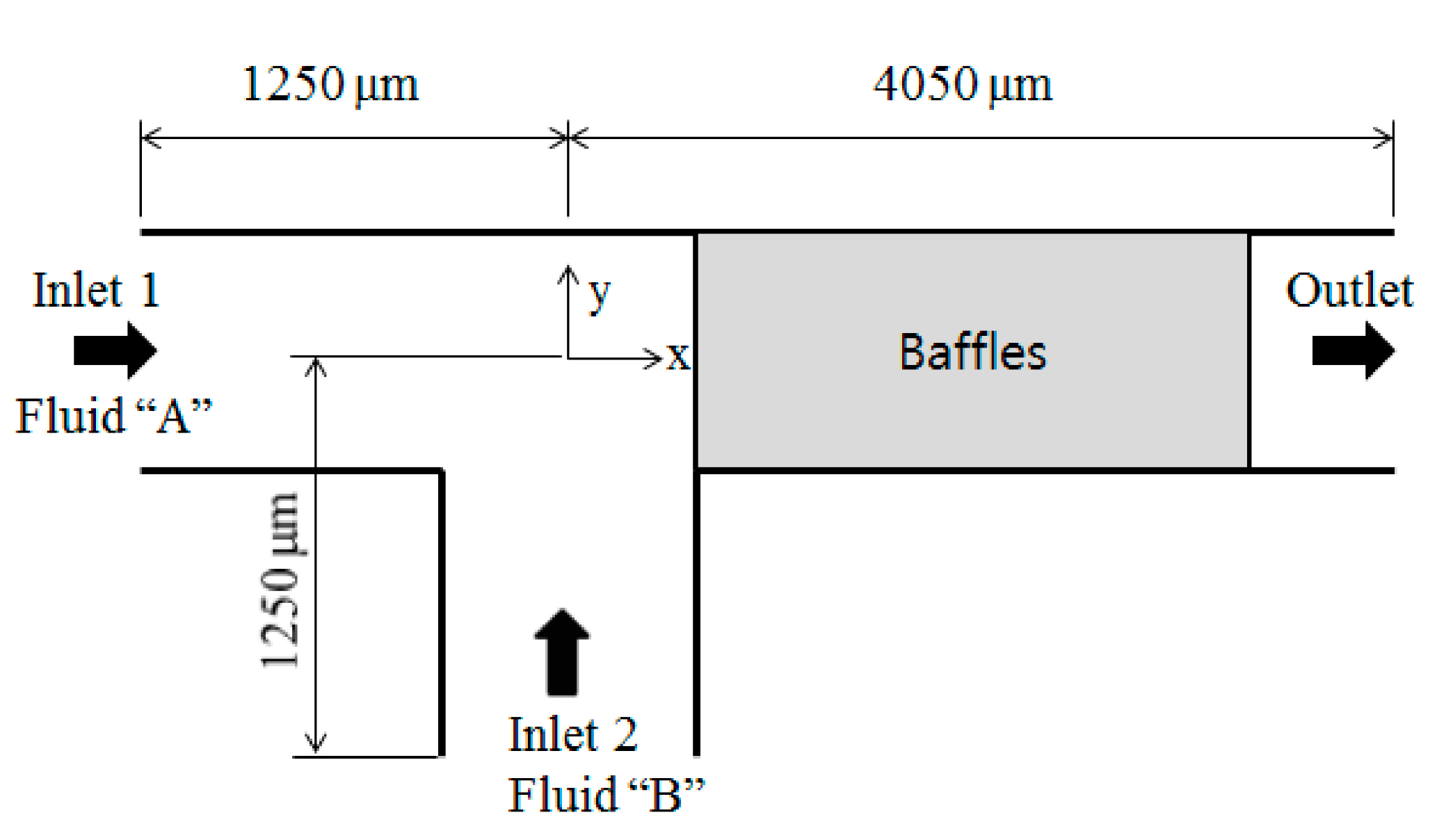
The overall layout of a T-shaped microchannel with three branches is shown in Figure 1. All three branches have a rectangular cross section that is 200 μm high by 120 μm deep. Inlet 1 and inlet 2 are both 1250 μm long, and they are called inlet branches. The branch after the junction of two inlets, including the baffle region, is called the outlet branch and is 4050 μm long. A certain number of baffles are to be placed in the baffle region. All baffles have a certain thickness, in reality. However, they were modeled as having zero thickness. The reason for this is explained in the Section 4. 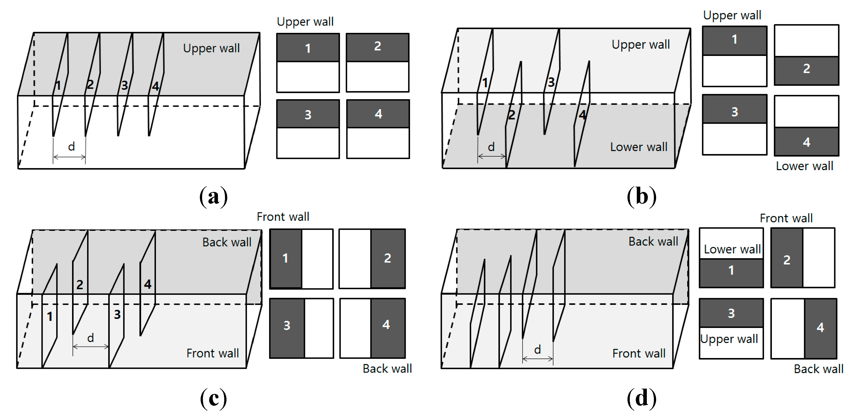Figure 2 shows four different baffle attachment configurations. The numbered rectangles in the figures are baffles. Four side walls are also designated in the figures. Figure 2a shows four baffles attached along the upper wall of the channel, which is called the upper wall attachment. Figure 2b,c shows two opposite wall attachments. The baffles in Figure 2b are attached by turns to the upper and lower walls of the channel, while they are alternately attached to the front and back walls of the channel in Figure 2c. Figure 2d shows a cyclic attachment of baffles to the four side walls of the channel. They are attached to the lower, front, upper, and back side walls of the channel in a cyclic order as shown in the figure. Four baffles make up one cycle. As the baffles have no geometric conflict in the z-direction, no special techniques are required to assemble it. For example, Sotowa et al. [17] showed a technique to assemble a microchannel with baffles and indentations.

For the sake of simplicity, we assumed the same aqueous solution flows into the two inlets. The fluid was assumed to have the properties found in many existing BioMEMS systems. Its diffusion constant is equal to D = 10⁻¹⁰ m²/s and the kinematic viscosity of fluid is ν = 10⁻⁶ m²/s at room temperature. This value of the diffusion constant is typical of small proteins in an aqueous solution. Thus, the Schmidt (Sc) number defined as the ratio of the kinetic viscosity and the mass diffusion of fluid is 10⁴.

Figure 1. Schematic diagram of a T-shaped micro-channel.

Figure 1. Schematic diagram of a T-shaped micro-channel.

Figure 2. Schematic diagrams of four different configurations of repeated baffles. (a) Upper wall attachment. (b) Opposite wall attachment: type 1. (c) Opposite wall attachment: type 2. (d) Cyclic attachment.

Figure 2. Schematic diagrams of four different configurations of repeated baffles. (a) Upper wall attachment. (b) Opposite wall attachment: type 1. (c) Opposite wall attachment: type 2. (d) Cyclic attachment.

3. Governing Equations and Computational Procedure

The fluid is assumed to be Newtonian and incompressible, and the equations of motion are the Navier-Stokes and continuity equations:

$$(\overrightarrow{u}\cdot \nabla )\overrightarrow{u}=-\frac{1}{\text{ρ}}\nabla p+\text{ν}{\nabla }^2\overrightarrow{u}$$

(1)

$$\nabla \cdot \overrightarrow{u}=0$$

(2)

where $\overrightarrow{u}$ is the velocity vector, p is the pressure, ρ is the mass density, and ν is the kinematic viscosity. The evolution of the concentration is computed from the advection diffusion equation:

$$(\overrightarrow{u}\cdot \nabla )\mathrm{\varphi }=D{\nabla }^2\mathrm{\varphi }$$

(3)

where D is the diffusion constant and ϕ is the local concentration or mass fraction of a given species.

The governing equations (Equations (1)–(3)) were solved using the commercial software, Fluent 14.5. All of the convective terms in Equations (1) and (3) were approximated by means of a QUICK (quadratic upstream interpolation for convective kinematics) scheme whose theoretical accuracy is third-order.

The two inlets were assumed to have a uniform velocity profile of 1 mm/s. The outflow condition is used at the outlet. Thus, the fluid flow in the microchannel corresponds to a Reynolds number of 0.3. All of the other walls were treated as no-slip walls. The mass fraction of the fluid at inlet 1 is set to ϕ = 0, and the fluid entering through inlet 1 is called fluid A. The fluid at inlet 2 has a mass fraction of ϕ = 1 and is called fluid B. Thus, c was defined as the mass fraction of the fluid B.

All the numerical solutions were evaluated in terms of the DOM, which is defined by Glasgow et al. [5]. The DOM was calculated using the following relation:

$$\text{DOM}=1-\frac{1}{\text{ξ}}\sqrt{{\displaystyle \sum _{i=1}^n\frac{{(c_i-\text{ξ})}^2}{n}\frac{u_i}{u_{\text{mean}}}}}$$

(4)

where u_i is the velocity in the i-th cell, u_mean is the mean velocity at the outlet of the microchannel, c_i is the mass fraction in the i-th cell, and n is the number of cells. ξ is specified as 0.5, which is the targeted case of equal mixing of the two reagents.

The computational domains shown in Figure 1 and Figure 2 were divided by means of structured hexahedral cells. All of the side sizes of each computational cell are equally long. All cells in the computational domain were made with all sides 5 μm long. A detailed study of the grid independence of numerical solutions was carried out in a previous study [8]. According to the results, the total mass flow rate at the outlet has an accuracy of 0.1% for a cell in which all sides are 10 μm long. For the case of a baseline design without any baffle, the DOM calculated at the section of x = 3 mm is 0.12, which is the same value reported by Glasgow et al. [5].

4. Results and Discussion

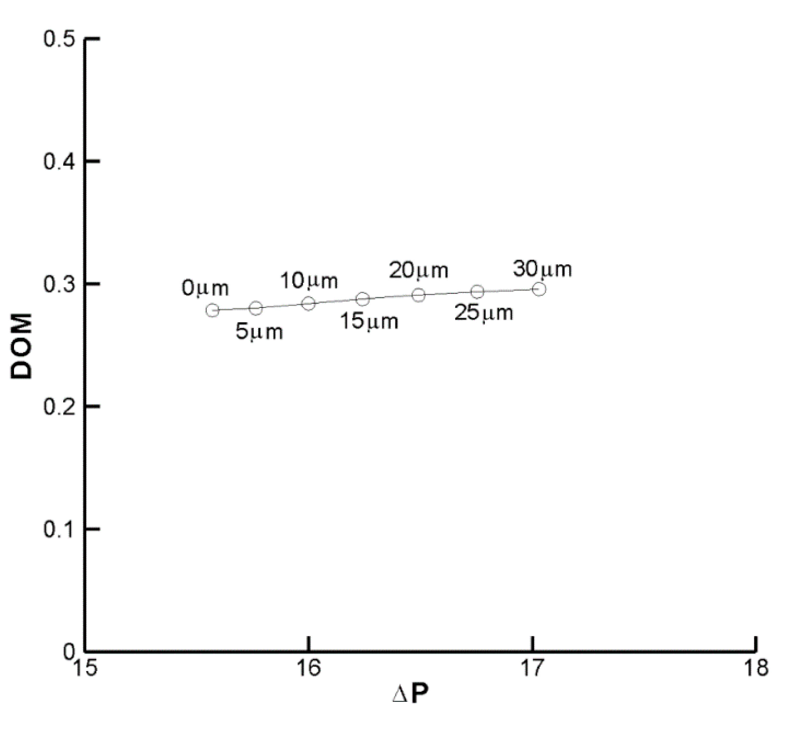
The effects of baffle thickness were first studied by simulating a cyclic configuration of 8 baffles. The baffles are 100 μm high and 120 μm deep fixed, while its thickness varies in the range of 0–30 μm. The distance between two consecutive baffles is 100 μm. Figure 3 shows the computed DOM as a function of pressure difference and baffle thickness. The DOMs were measured at the outlet, and the pressure difference was determined as the higher value between the two inlets and outlet. The DOM increases with the baffle thickness at the expanse of the pressure load. However, the effects of baffle thickness are negligibly small compared with the effects of baffle configuration which are studied in this paper. Furthermore, the relationship is simply linear, meaning that a baffle with zero thickness is a good model for thin baffles. It is also helpful to focus and/or isolate the only effects of baffle configuration. Thus, all baffles were modelled as having zero thickness in this paper.

Figure 3. Effects of baffle thickness on the DOM.

Figure 3. Effects of baffle thickness on the DOM.

To study the effect of baffle configuration on the DOM, four different configurations shown in Figure 2 were computed for the same flow condition. The mean velocities at the two inlets were specified as 1 mm/s. The baffles were inserted to block one half of the cross section where they were attached. For example, the baffle attached to the upper wall is 100 μm high and 120 μm deep. Each baffle is located 100 μm apart from neighboring baffles in the main stream direction.

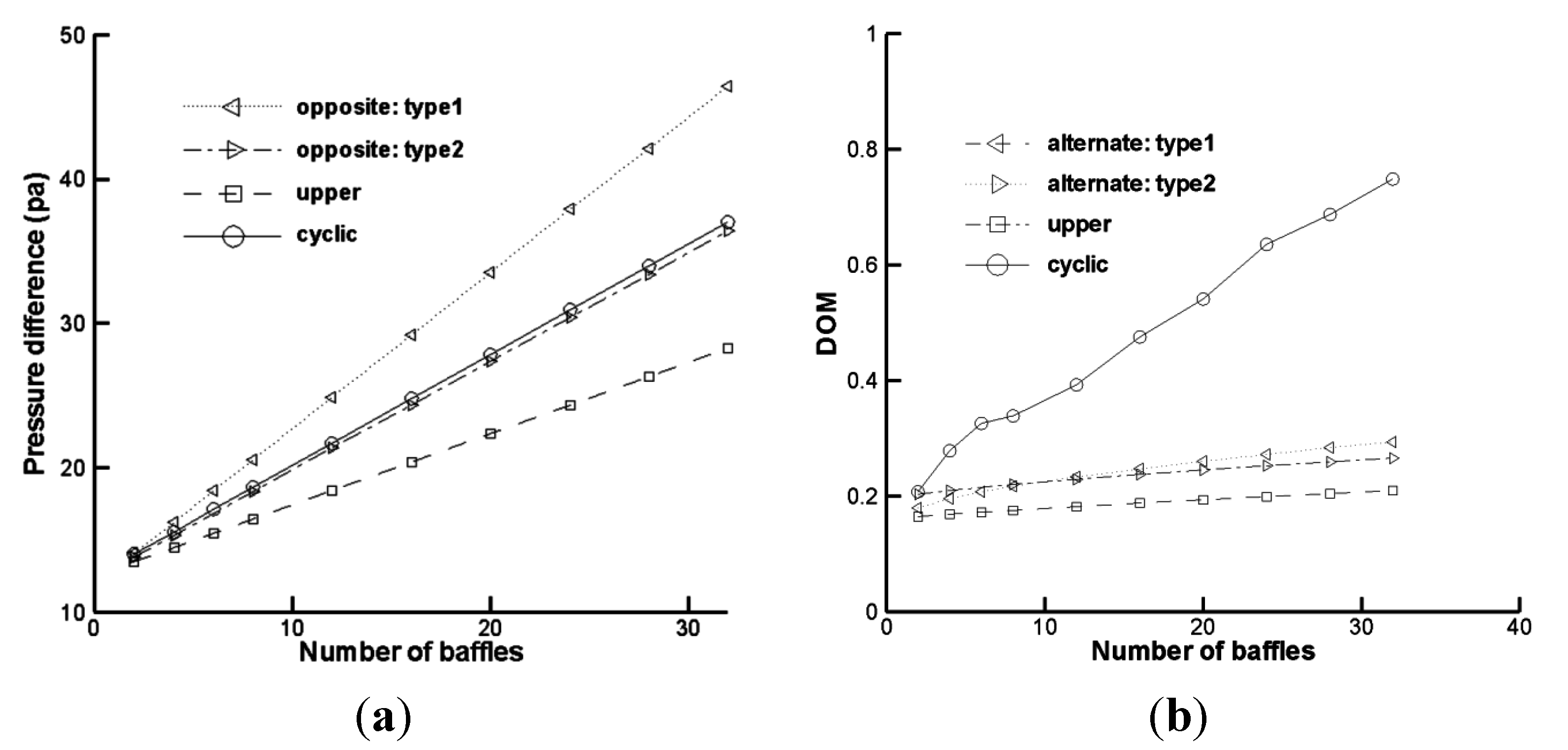
Figure 4 shows the computed variation of the pressure difference and the DOM with the number of baffles. The pressure difference shows a linear relationship with the number of baffles, but its slope shows some dependence on the baffle configuration. The DOM as a function of the number of baffles exhibits very different behavior. The upper wall attachment shows the worst behavior in terms of the DOM with the number of baffles. Similar behavior was obtained when the baffles were attached to the lower wall instead of the upper wall. This means the upper wall attachment is a typical kind of one-wall attachment. The two opposite wall configurations show almost identical DOM behavior with respect to the number of baffles. Conversely, the cyclic configuration shows a remarkable improvement compared to the other cases. The DOM of the cyclic configuration is several times larger than those of the other cases.

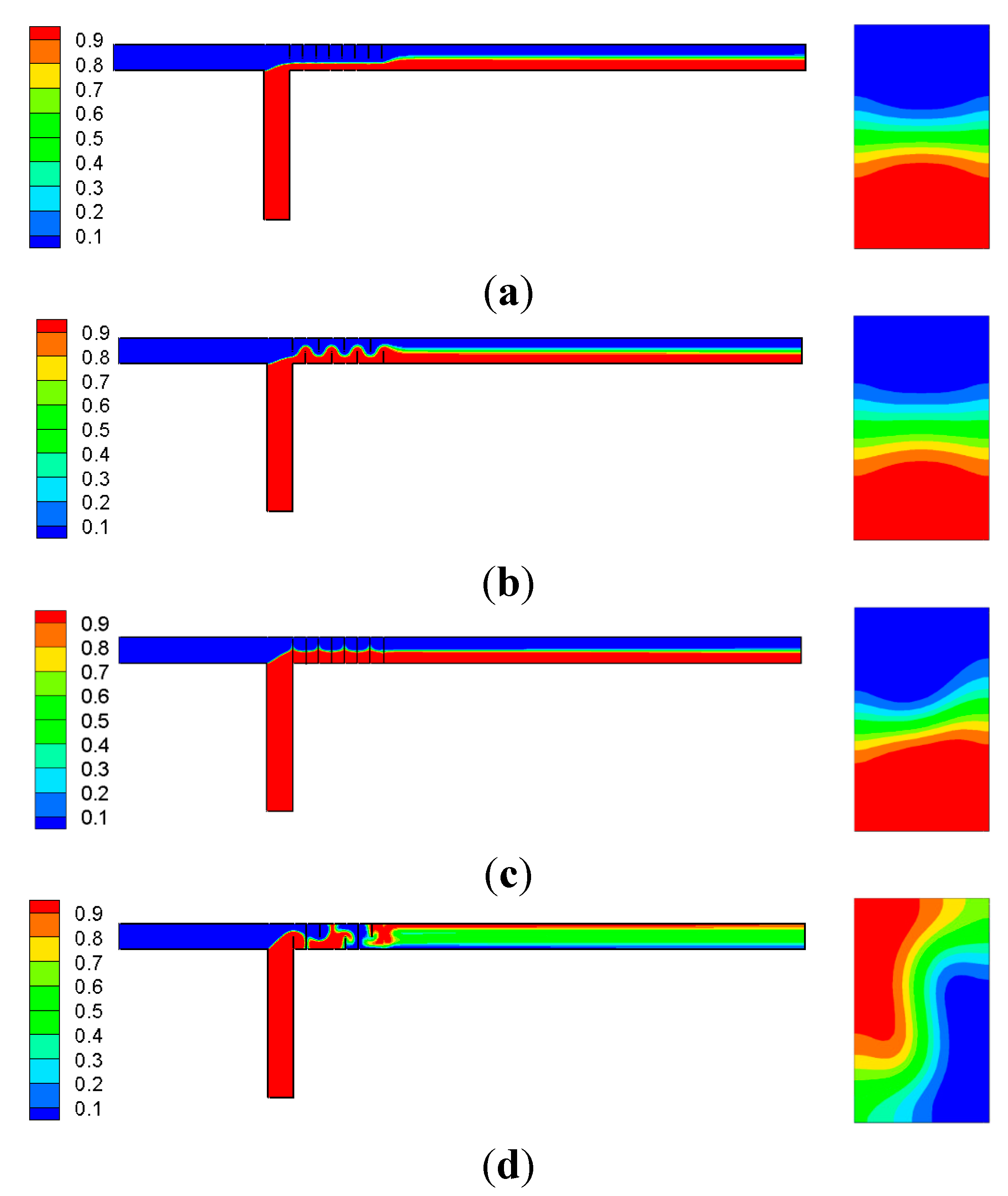
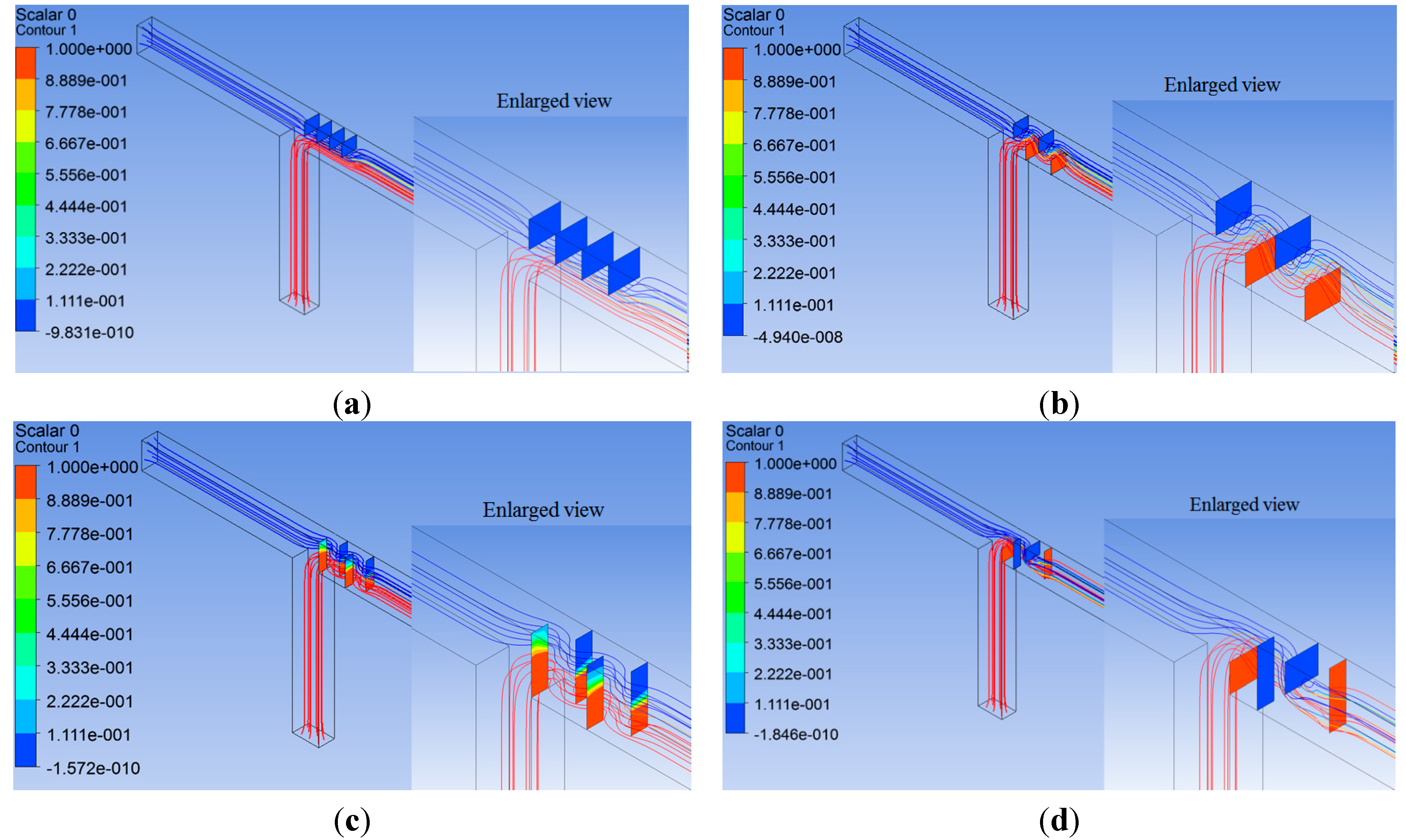
To understand how the mixing enhancement of the cyclic attachment is achieved, a set of computations was carried out for four configurations made of eight baffles. The resulting mass fraction contours are compared in Figure 5. The left contours in each figure show the mass fraction of the fluid B along the central plane of the channel, while the contours on the right-hand side is at the cross section of outlet. The mass fraction contours of the cyclic configuration show the most vigorous mixing in the baffle region. As a result, the contours of the mass fraction at the outlet cross section are completely different from the other cases. The boundary between the two fluids A and B is rotated from the horizontal to the diagonal direction, and the boundary shape is more curved than the other cases. This angular movement in the cross section of the channel seems to cause the aforementioned mixing enhancement. The role of baffles can be seen clearly in Figure 6, which shows the streamline pattern around the baffles. When the baffles are placed in a cyclic order, the flow has to rotate and twist as it passes though the baffles, unlike other cases. For example, the flow in the upper attachment is simply pushed down without any noticeable mixing as it passes through the baffles.

Figure 4. Variation of pressure difference and its relationship with the DOM. (a) Pressure difference vs. number of baffles. (b) DOM vs. number of baffles.

Figure 4. Variation of pressure difference and its relationship with the DOM. (a) Pressure difference vs. number of baffles. (b) DOM vs. number of baffles.

Figure 5. Comparison of the mass fraction contours of fluid “B” along the central plane. (a) Upper wall attachment. (b) Opposite wall attachment: type 1. (c) Opposite wall attachment: type 2. (d) Cyclic attachment.

Figure 5. Comparison of the mass fraction contours of fluid “B” along the central plane. (a) Upper wall attachment. (b) Opposite wall attachment: type 1. (c) Opposite wall attachment: type 2. (d) Cyclic attachment.

Figure 6. Comparison of the streamline patterns and vorticity distributions around the baffles. (a) Upper wall attachment. (b) Opposite wall attachment: type 1. (c) Opposite wall attachment: type 2. (d) Cyclic attachment.

Figure 6. Comparison of the streamline patterns and vorticity distributions around the baffles. (a) Upper wall attachment. (b) Opposite wall attachment: type 1. (c) Opposite wall attachment: type 2. (d) Cyclic attachment.

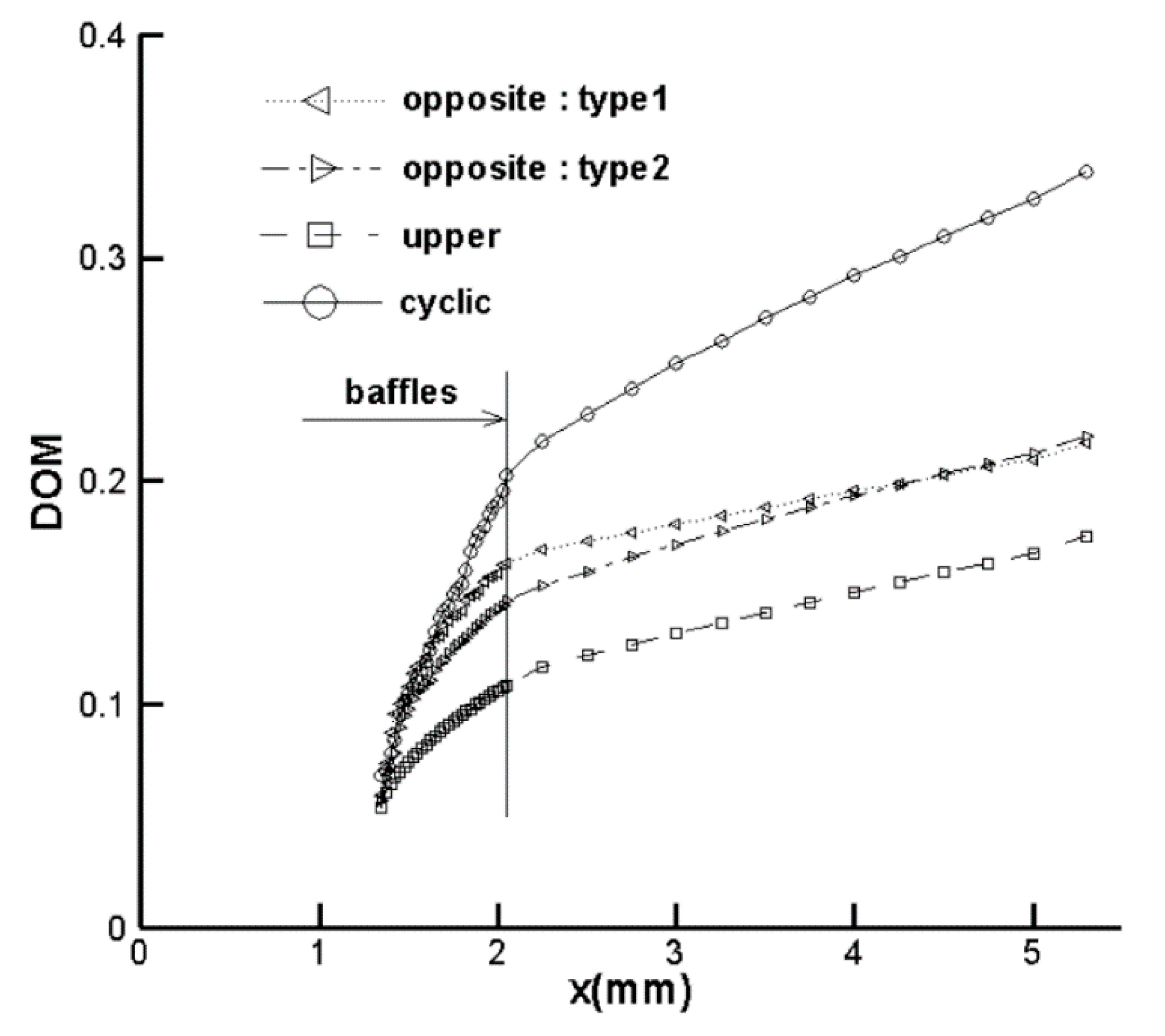
The DOM evolutions along the outlet branch for four configurations are plotted in Figure 7. The figure shows that the mixing enhancement of the cyclic attachment is achieved in two different ways. One enhancement occurs in the baffle region. The cyclic attachment shows a DOM improvement of about 87%, just after the baffle region, compared to that of the upper wall arrangement of baffles. This improvement appears to be due to the rotation and twist of the flow in the cross section of the channel, as shown in Figure 5 and Figure 6. 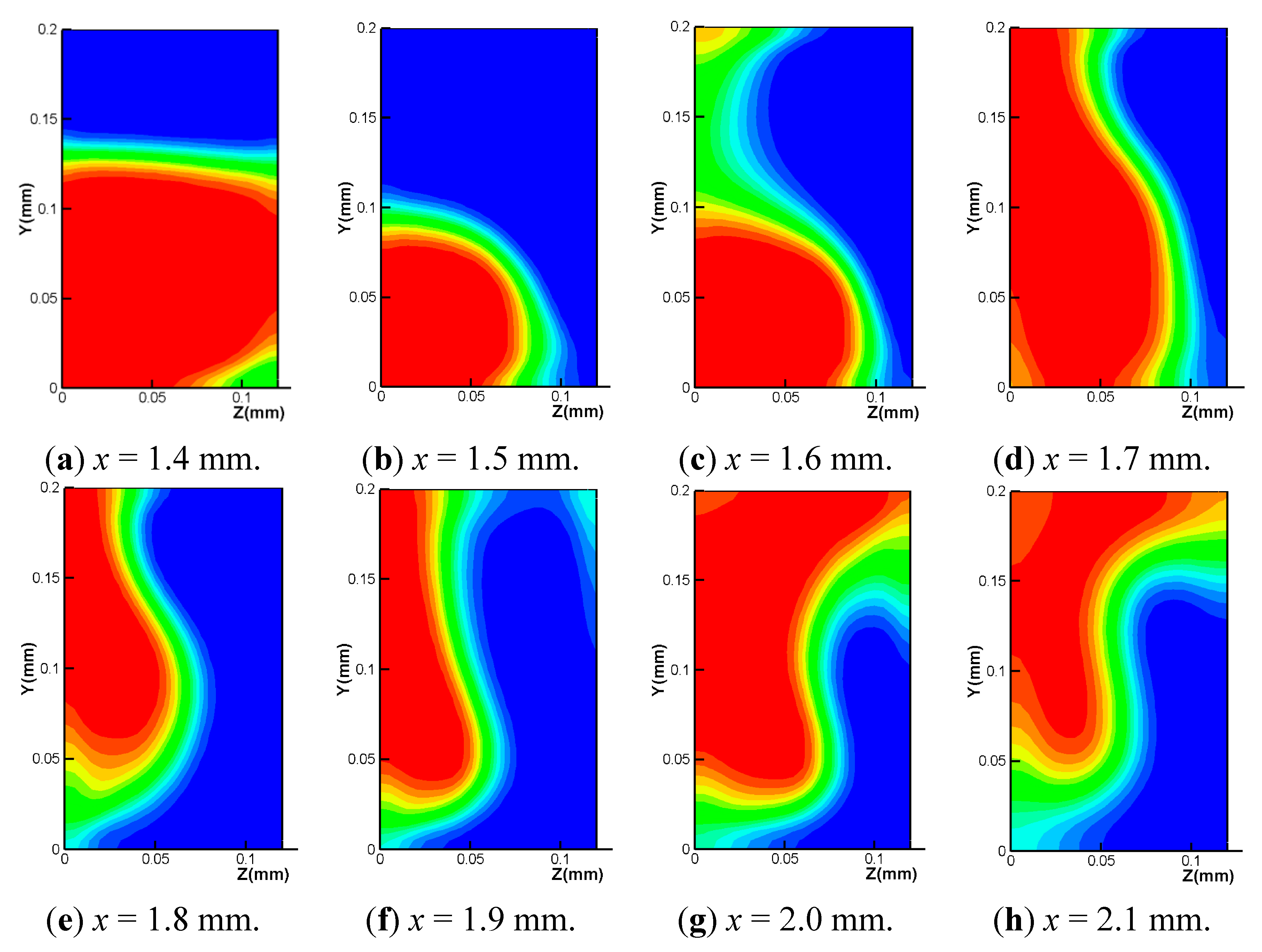Figure 8 shows how the mass fraction distribution of fluid B changes as the flow passes through the eight baffles. For example, Figure 8a depicts the mass fraction distribution in the mid plane between the first and second baffles. In the same way, Figure 8g shows the result obtained in the mid plane between the seventh and eighth baffles, and Figure 8h is in the plane of 50 μm downstream of the eighth baffle. Fluid B (shown in red in the figures) is seen to rotate by more than 90° in the clockwise direction. This flow rotation was not observed in the other configurations. As a result, the boundary between fluids A and B became more blurred and curved as the fluid flow passed through the baffles. The other improvement occurs in the remaining section of the outlet branch. As shown in Figure 7, the slope of the cyclic attachment is about twice as steep as the other slopes. The mixing in this region is due entirely to the molecular diffusion. Therefore, the shape and length of the boundary between fluids A and B seem to determine the DOM evolution rate in this region. The cyclic configuration exhibits the longest and most curved boundary as shown in Figure 5.

Figure 7. Comparison of the DOM evolutions along the outlet branch.

Figure 7. Comparison of the DOM evolutions along the outlet branch.

Figure 8. Development of the DOM distributions throughout the baffle region.

Figure 8. Development of the DOM distributions throughout the baffle region.

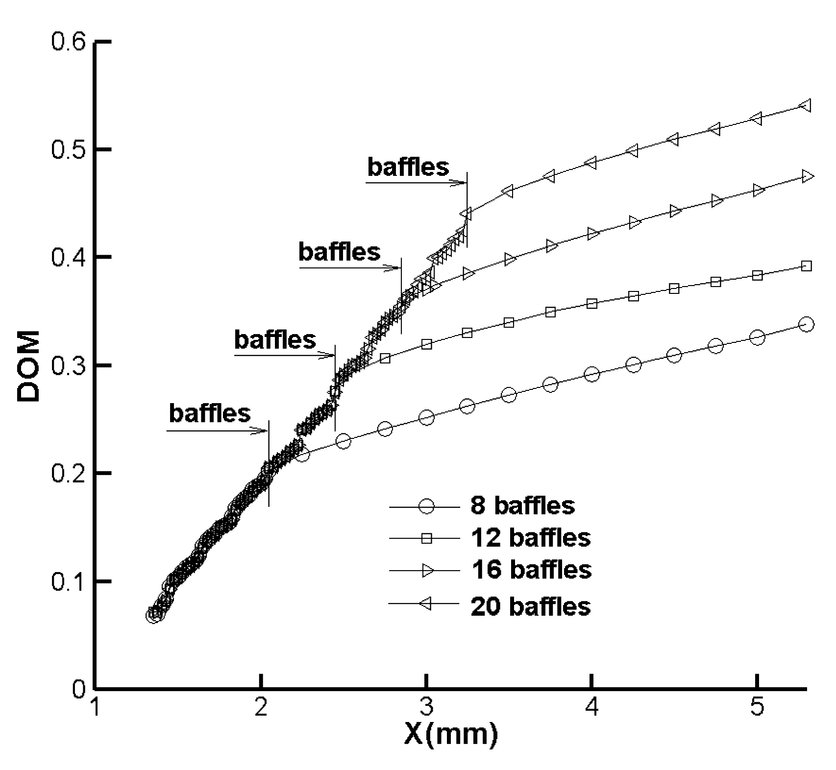
The mixing characteristics of the cyclic configuration were studied further by varying the number of baffles from 8 to 20. Figure 9 shows the DOM evolutions along the outlet branch. The figure shows that almost the same amount of DOM increase is achieved when the baffles are increased by a multiple of four. Thus, the DOM increase within the baffle region seems entirely due to the baffle configuration. This suggests that the DOM increase within the baffle region is proportional to a multiple of four baffles, while the DOM distribution after the baffle region has almost a constant evolution rate.

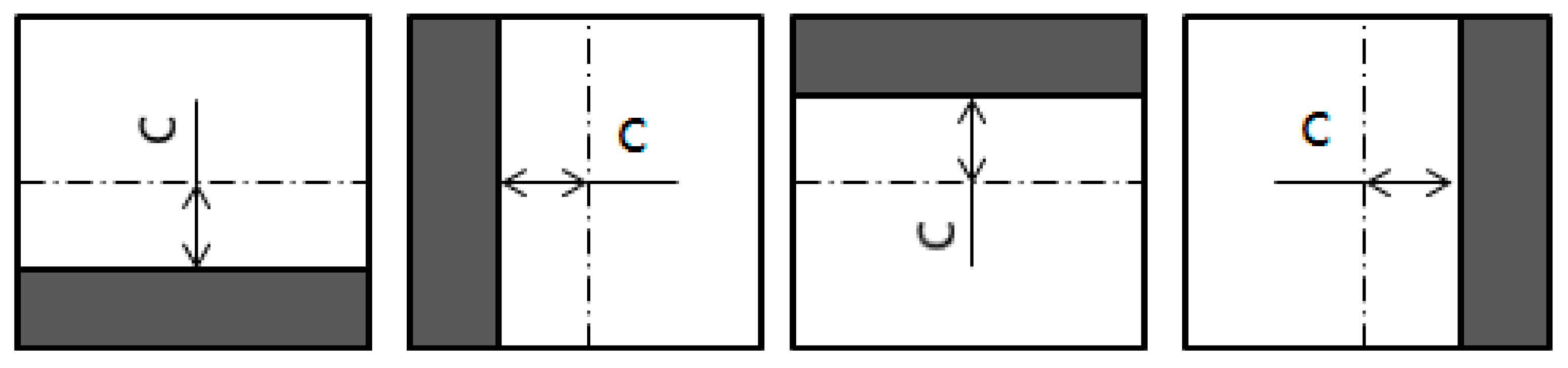
The cyclic configuration of the baffles was studied further by examining the effects of two major geometric parameters: the clearance gap c and the baffle interval d. Figure 10 shows four cross sections where a baffle (shaded region in the figure) is attached to one of the four side walls. For example, a baffle is attached to the bottom wall of the cross section in Figure 10a. The clearance gap between the centerline and the baffle edge, shown as c in Figure 10, seems to be an important geometric parameter to be optimized. A set of computations was carried out. The clearance gap c was varied over a range of −20 to 30 μm while the baffle interval d was kept unchanged at 100 μm. Here a negative (−) clearance gap means that the baffle is larger than one half of the channel height or width.

Figure 9. Comparison of the DOM evolutions for four different numbers of baffles.

Figure 9. Comparison of the DOM evolutions for four different numbers of baffles.

Figure 10. Definition of clearance gap c.

Figure 10. Definition of clearance gap c.

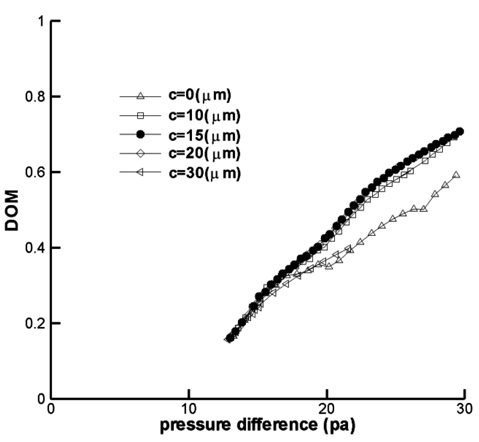
Figure 11 shows the DOM distribution as a function of the pressure difference for five different clearance gaps. The clearance gap c is seen to be optimized in terms of the DOM. The optimal value is about 15 μm. This optimization can be explained as follows. As the clearance gap c increases, the baffles become smaller and some additional baffles might be used for a given pressure load. More baffles may lead to an increase in the DOM. However, smaller baffles may not properly block the flow and do not promote mixing in the baffle region. Thus, we can expect that there is an optimal value of the clearance gap c for a given pressure load.

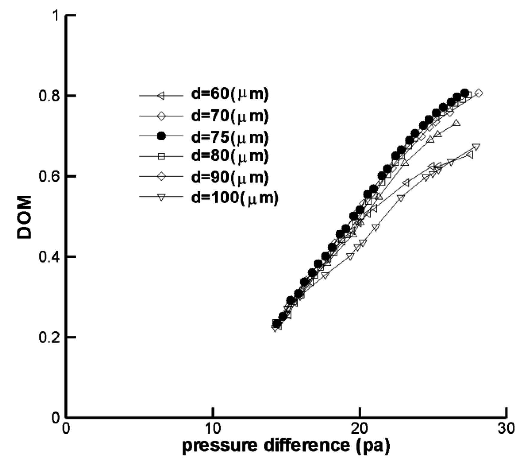
The baffle interval, shown as d in Figure 2, is another geometric parameter to be optimized. Its effect on the DOM was studied by varying its value over a range of 60 to100 μm while the clearance gap c was kept unchanged at 15 μm. Figure 12 shows the effects of the baffle interval on the DOM distribution for five different baffle intervals. The baffle interval is also seen to be optimized in terms of the DOM. The optimal baffle interval is about 75 μm for a given configuration and flow conditions.

Figure 11. Effects of the clearance on the DOM relationship with pressure difference.

Figure 11. Effects of the clearance on the DOM relationship with pressure difference.

Figure 12. Effects of the baffle interval on the DOM relationship with pressure difference.

Figure 12. Effects of the baffle interval on the DOM relationship with pressure difference.

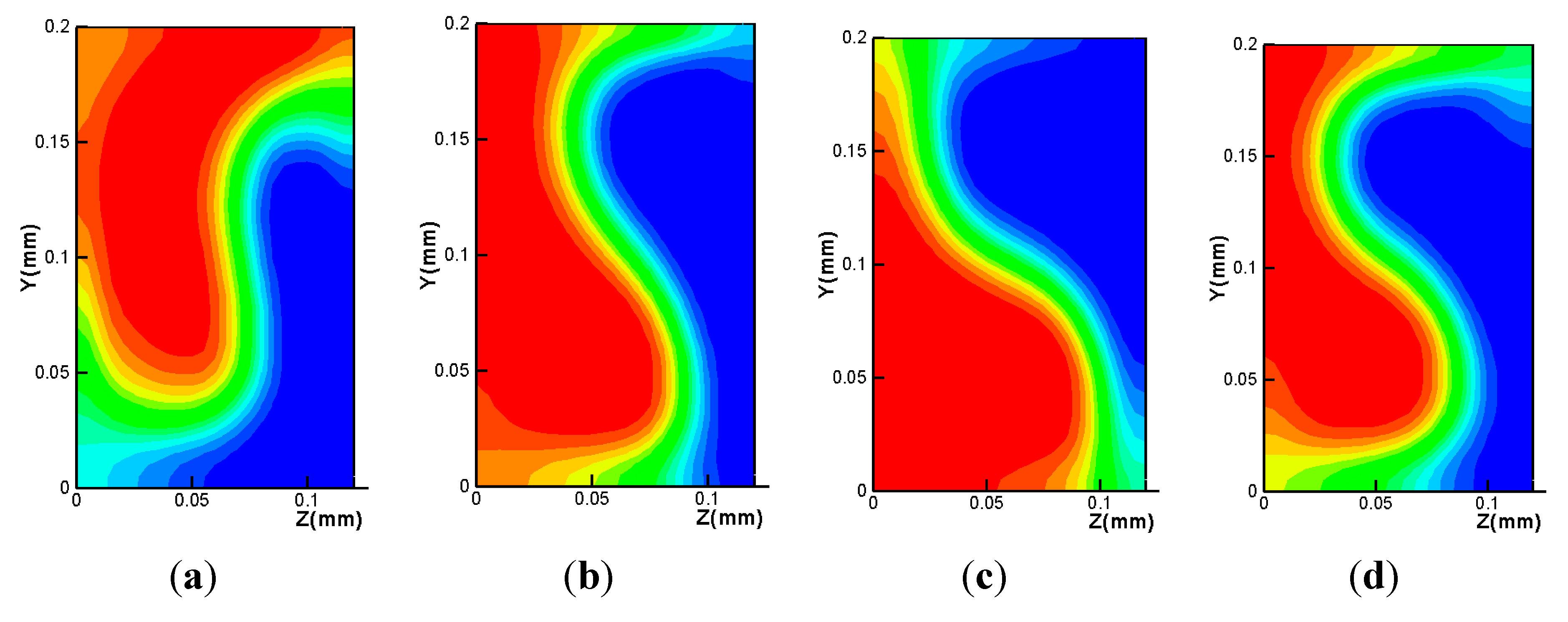
To understand how the baffle size affects the mixing of two fluids, A and B, the mass fraction distributions obtained with three different baffle sizes and two baffle intervals are depicted in Figure 13. The cross section is located 50 μm downstream of the eighth baffle. Figure 13a–c shows how the boundary between fluids A and B changes as the baffle clearance gap is optimized. Figure 13d is the mass fraction distribution of the baffle configuration optimized in terms of the baffle interval as well as the clearance gap. The boundary between fluids A and B is the longest curve, and it is a result of the flow rotation in the y-z plane as the flow passes through the baffles. 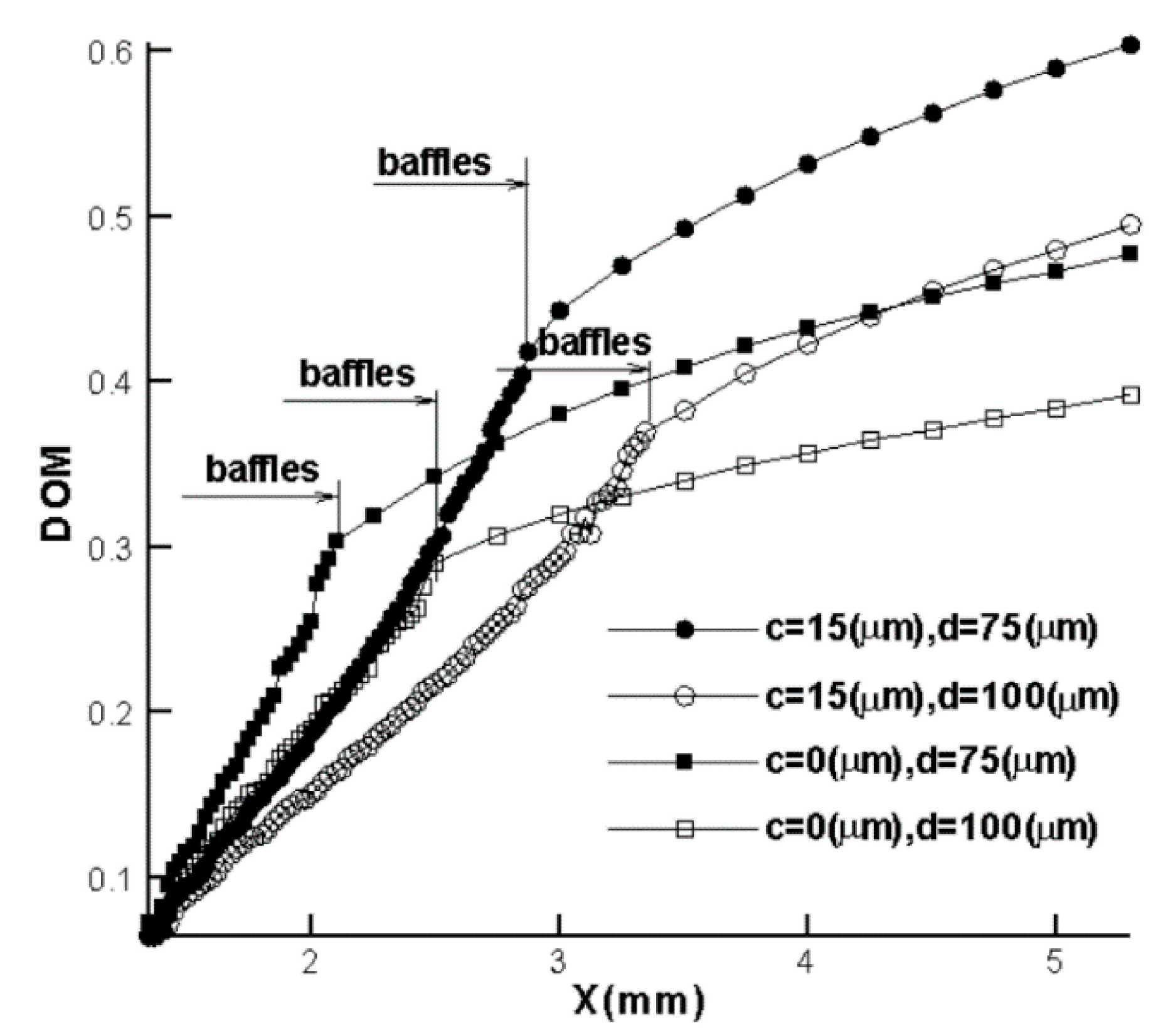Figure 14 shows how the baffle size and interval affects the DOM evolution in the outlet branch. All four cases correspond to a similar pressure load between the inlet and outlet sections. For c = 0 μm and d = 100 μm, twelve baffles were used and the pressure load was 21.70 Pa. For c = 15 μm and d = 100 μm, 21 baffles were used and the pressure load was 21.59 Pa. Twenty baffles were used for c = 15 μm and d = 75 μm, and the corresponding pressure load was 21.64 Pa. The DOM within the region of the baffles is affected by both the baffle clearance gap and the baffle interval, while the DOM evolution rate after the region of the baffle is mainly affected by the baffle clearance gap. The configuration made of 20 baffles with c = 15 μm and d = 75 μm shows the best DOM, and it suggests that we can find an optimum baffle configuration for a given pressure load.

Figure 13. Comparison of the mass fraction distribution in the cross section at 50 μm downstream of baffles for four different baffle clearances and intervals. (a) c = 0 μm and d = 100 μm. (b) c = 15 μm and d = 100 μm. (c) c = 25 μm and d = 100 μm. (d) c = 15 μm and d = 75 μm.

Figure 13. Comparison of the mass fraction distribution in the cross section at 50 μm downstream of baffles for four different baffle clearances and intervals. (a) c = 0 μm and d = 100 μm. (b) c = 15 μm and d = 100 μm. (c) c = 25 μm and d = 100 μm. (d) c = 15 μm and d = 75 μm.

Figure 14. Comparison of DOM evolution along the outlet branch.

Figure 14. Comparison of DOM evolution along the outlet branch.

5. Conclusions

In this paper, the effects of baffle configuration on the mixing performance of a T-shaped microchannel of rectangular cross section were numerically studied. The performance of the T-shaped microchannel was studied by examining the DOM and the pressure load between the inlet and outlet sections. All numerical computations were performed with Fluent 14.5 commercial software.

Four baffle configurations (upper, opposite (type1), opposite (type2), and cyclic) were designed and simulated in order to study the effects of configuration on the mixing performance of the microchannel. A cyclic baffle configuration means that four baffles are attached to the four sides of the microchannel wall in a cyclic order. A comparison of the DOM distributions for four different baffle configurations shows that the baffle configuration is an important design parameter. When a cyclic configuration is used, the DOM at the outlet shows the best result with a value greater than twice that of the DOM for a corresponding upper wall configuration.

The DOM improvement of the cyclic configuration was found to be achieved in two different ways. One improvement was within the baffle region. For example, when eight baffles were used, the DOM of the upper wall configuration was about 0.1 at the end of the baffle region. The DOM at the same location was increased to about 0.2 for a cyclic configuration with eight baffles. This increase in the DOM seems to be caused by the flow rotation in the cross section as the flow passes through the baffles. The flow rotation means that the boundary between fluid A and B rotates in the clockwise direction. The other improvement is observed in the remaining outlet branch after the baffle region. Mixing in the outlet branch (without baffles) is entirely due to molecular diffusion, so an improved DOM means more vigorous diffusion. This vigorous diffusion seems to be caused by the distorted shape and extended length of the boundary between fluids A and B. The boundary shape of a cyclic configuration at the exit of the baffle region is almost like a letter S, whereas that of the upper configuration is like a circular arc with a large radius. Furthermore, the boundary of a cyclic configuration is more blurred and thicker than in the other cases.

The baffle size and its interval between two consecutive baffles were shown to be optimized in terms of the DOM. For the channel geometry considered in this paper, the optimal interval is about 75 μm and the optimal clearance gap is 15 μm.