
Invariant Observer-Based State Estimation for Micro-Aerial Vehicles in GPS-Denied Indoor Environments Using an RGB-D Camera and MEMS Inertial Sensors

Abstract
:
1. Introduction
2. Related Work
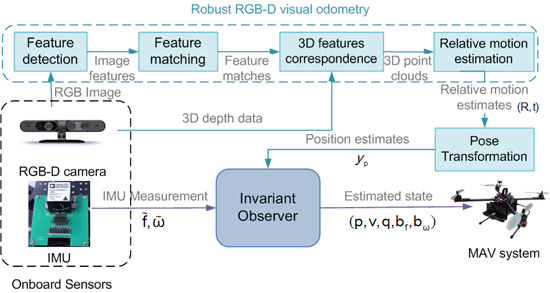
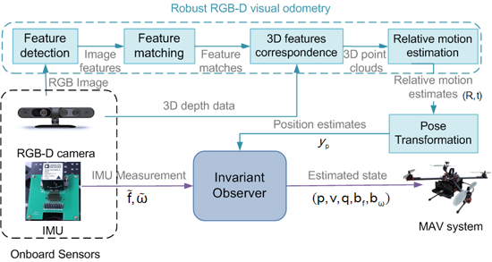
3. Overview of the RGB-D Visual/Inertial Navigation System Framework
4. Robust RGB-D Visual Odometry
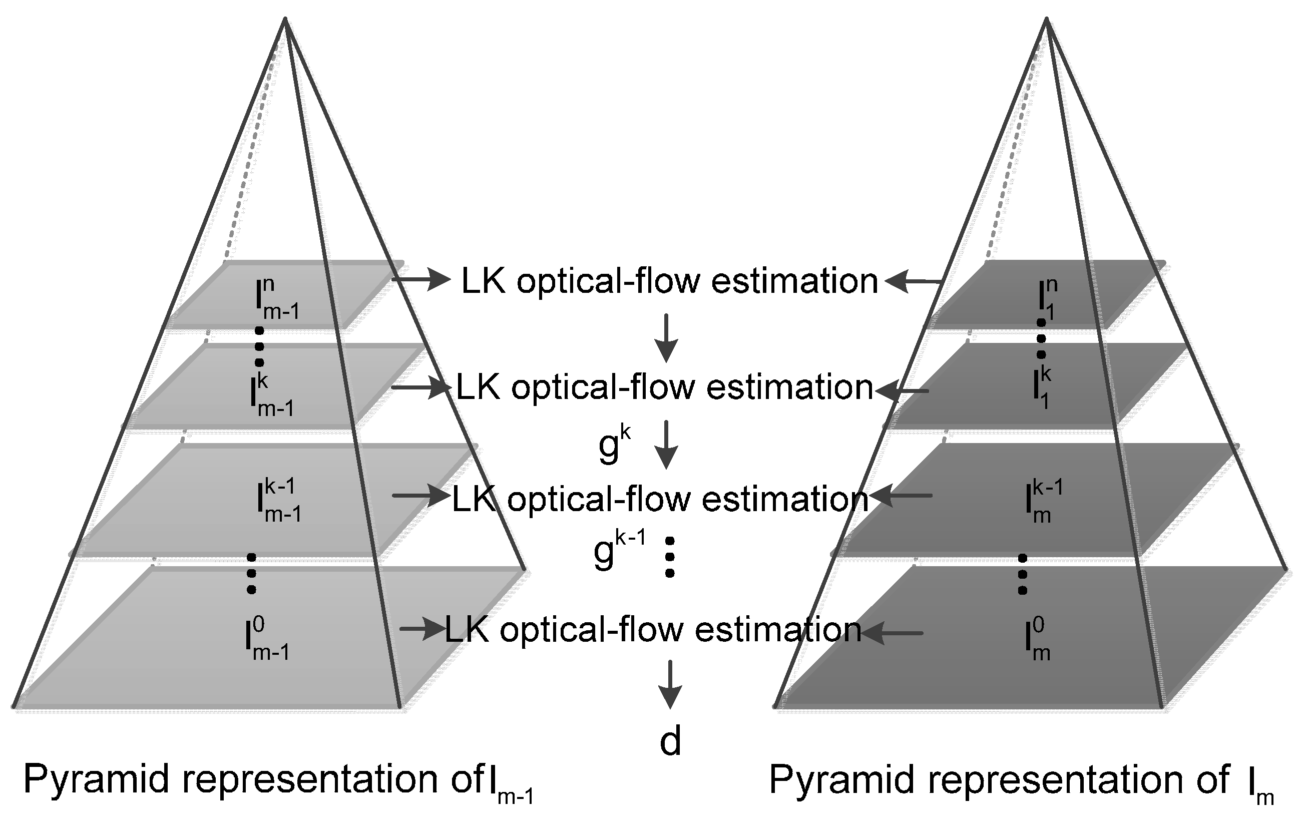
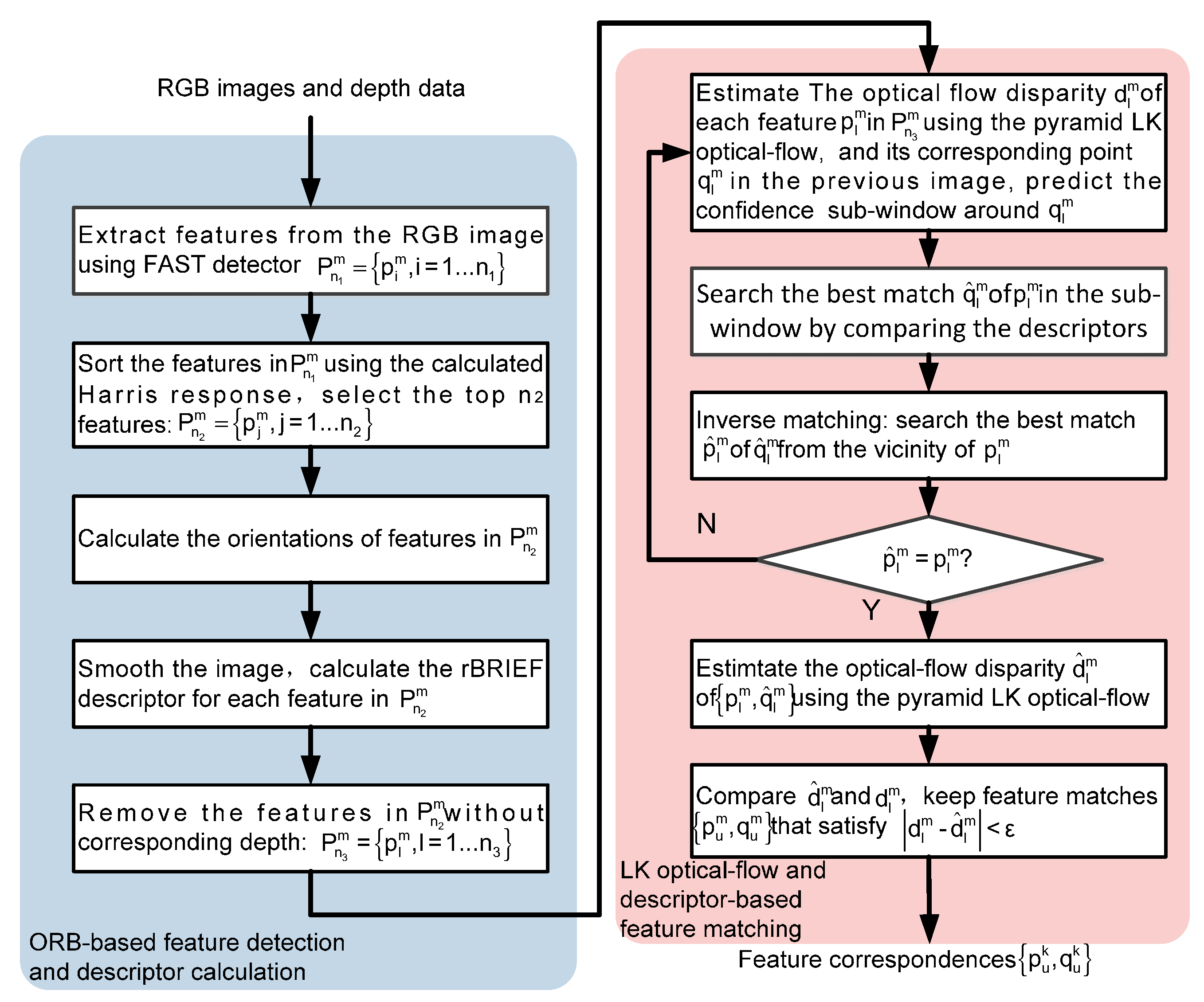
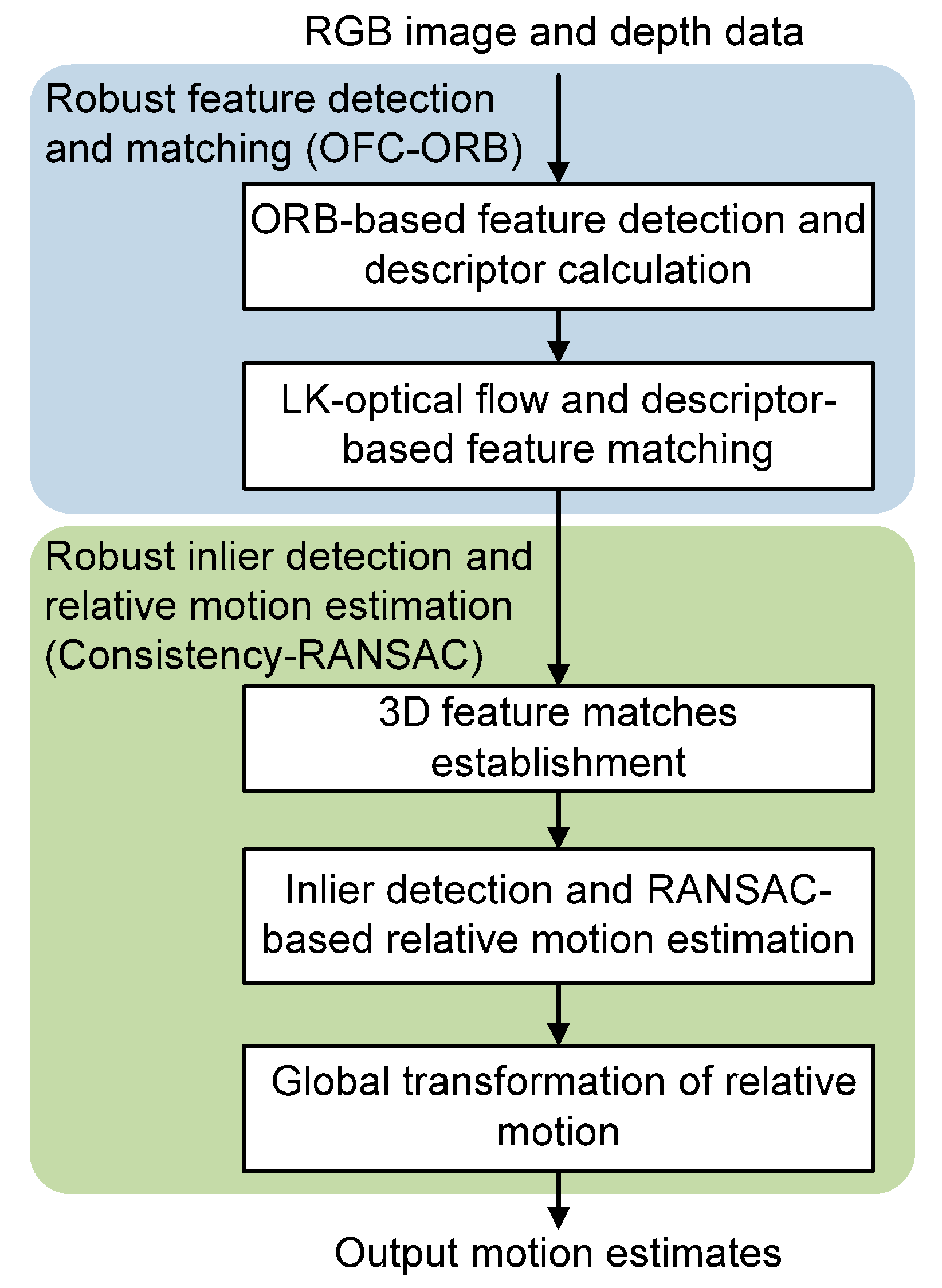
4.1. Robust Feature Detection and Matching

| Input | Two consecutive images captured by the RGB-D camera |
| Output | Feature correspondence set S of |
| 1 | Extract features from respectively, using the ORB detector, compute the descriptor for each feature of |
| 2 | Extract the depth data for each feature of , discard features that do not have corresponding depth, sort features in in an ascending order of the x-coordinates, obtain |
| 3 | Initialize the feature correspondence set |
| 4 | for each |
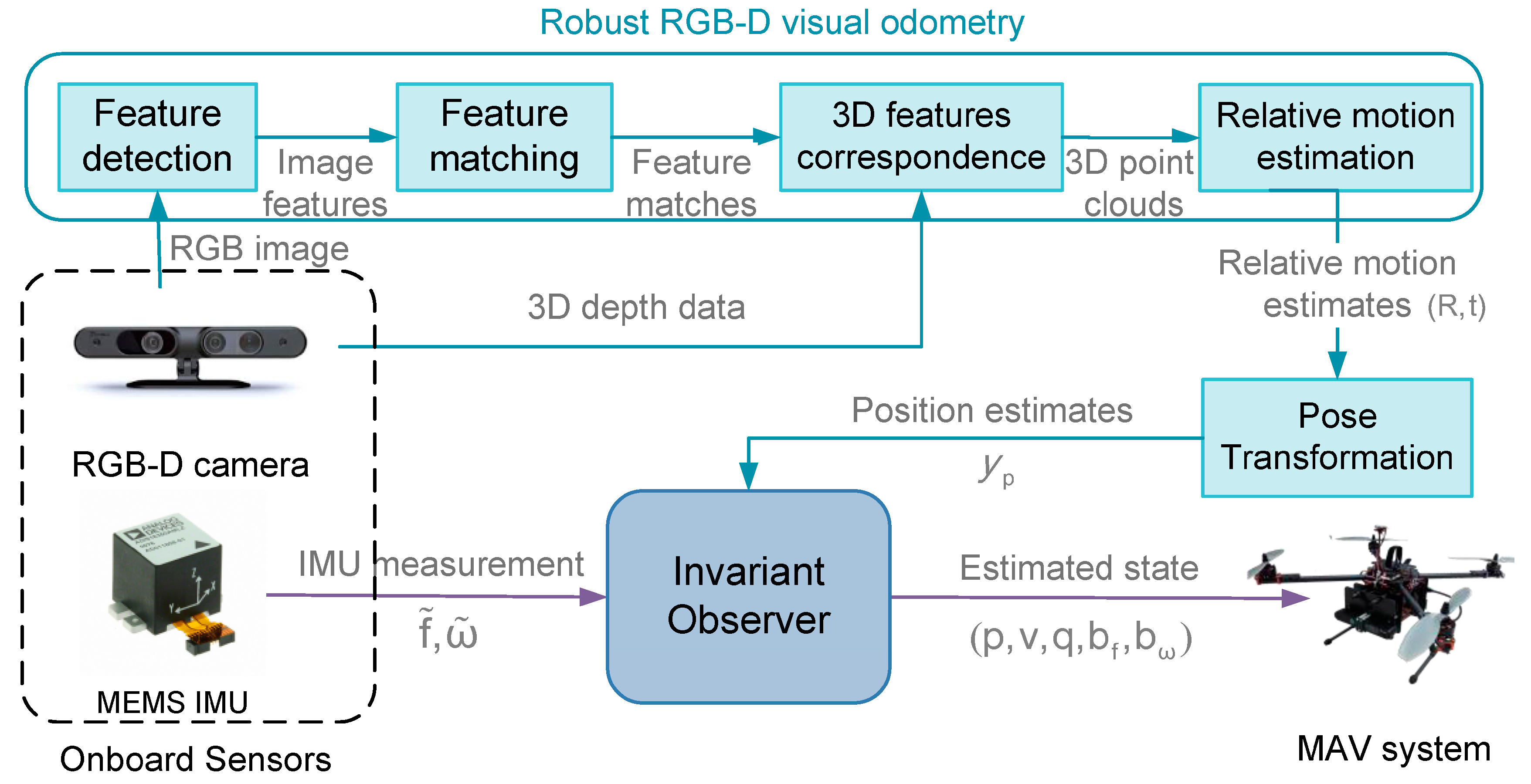
| 5 | Estimate the optical-flow vector of using the pyramid LK-optical-flow algorithm, calculate the corresponding point in : . |
| 6 | Build the confidence sub-window of size centered at |
| 7 | Find the best match of from , by searching for that satisfies: |
| 8 | Build a sub-window centered at in , find the best match of from |
| 9 | if |
| 10 | Estimate the optical-flow vector between |
| 11 | if |
| 12 | |
| 13 | end if |
| 14 | end if |
| 15 | end for |
| 16 | return S |
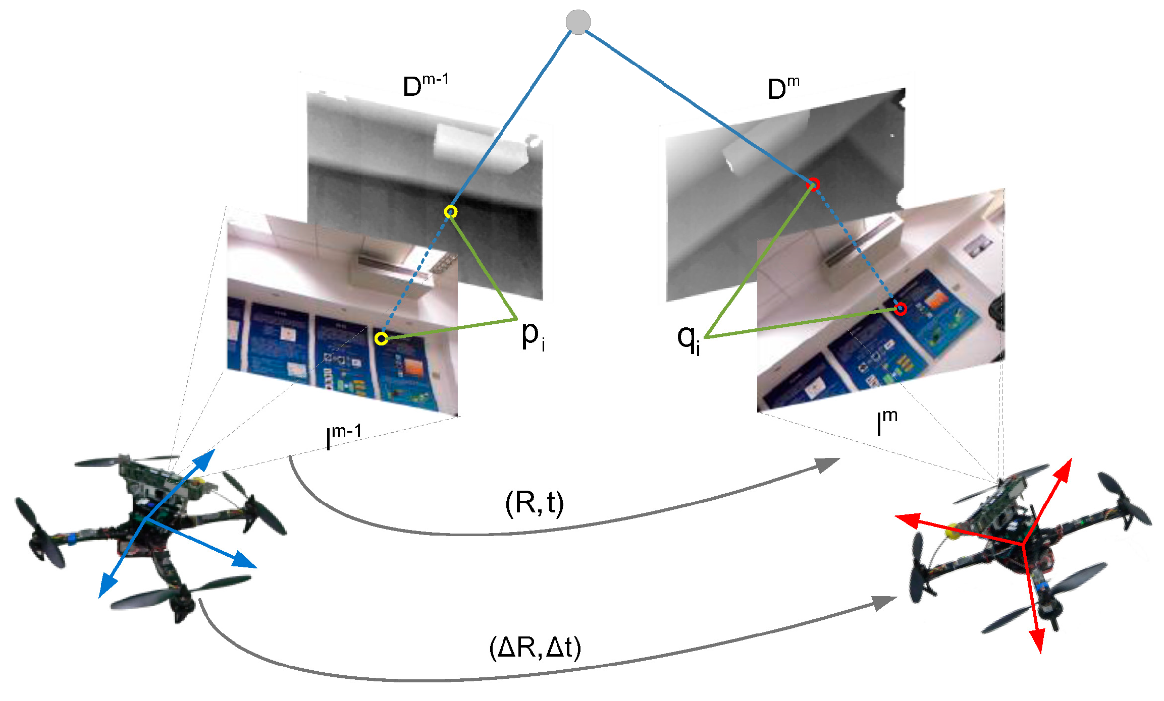
4.2. Robust Inlier Detection and Relative Motion Estimation

| Input | Two 3D point clouds with correspondences: |
| Output | Relative motion of |
| 1 | Calculate the centroid of |
| 2 | for i = 1 to n |
| 3 | |
| 4 | |
| 5 | end for |
| 6 | Sort the point set in the ascending order of : |
| 7 | Select the top n1 pairs of feature matches: |
| 8 | RANSAC initialization: , , |
| 9 | while do |
| 10 | Initialize the sample set and the jth consensus set: , |
| 11 | Randomly select pairs of feature matches from Q: |
| 12 | |
| 13 | Estimate that minimizes the error function given in Equation (17) based on SVD approach, using features in |
| 14 | for each AND do |
| 15 | if |
| 16 | |
| 17 | end if |
| 18 | end for |
| 19 | if |
| 20 | Re-estimate that minimizes the error function based on SVD approach, using features in the consensus set |
| 21 | for each do |
| 22 | |
| 23 | end for |
| 24 | |
| 25 | if |
| 26 | , |
| 27 | end if |
| 28 | if |
| 29 | break |
| 30 | end if |
| 31 | end if |
| 32 | |
| 33 | end while |
| 34 | return |
4.3. Global Transformation of Relative Motions
5. Invariant Observer Based State Estimation
5.1. Review of Invariant Observer Theory
- (a)
- ;
- (b)
- , i.e., the observer is invariant by the transformation group.
- (1)
- wi is the invariant frame. A vector field w: TX → X is G-invariant if it verifies:The invariant frame is defined as the invariant vector fields that form a global frame for TX. Therefore, forms a basis for TxX. An invariant frame can be calculated by:where υi ϵ TeX is a basis of υi ϵ TeX, and γ(x) is the moving frame. Following the Cartan moving frame method, the moving frame γ(x) can be derived by solving φg(x) = c for g = γ(x), where c is a constant. In particular, one can choose c = e such that γ(x) = x−1.
- (2)
- denotes the invariant output error, which is defined as follows:Definition 3.(Invariant output error) The smooth map is an invariant error which verifies the following properties:
- (a)
- For any , is invertible;
- (b)
- For any , ;
- (c)
- For any , ;
According to the moving frame method, the invariant output error can be given by: - (3)
- is the invariant of G, which verifies:Following the moving frame method, the invariant is obtained by:where γ(x) is the moving frame.
- (4)
- Li is a 1 × r observer gain matrix that depends on I and ε, such that:
- (a)
- is a diffeomorphism on X × X;
- (b)
- For any , ;
- (c)
- .
5.2. Sensor Measurement Models
5.3. RGB-D Visual/Inertial Navigation System Model
5.4. Observer Design of the RGB-D Visual/Inertial Navigation System
5.5. Calculation of Observer Gains Based on Invariant-EKF
6. Implementation and Experimental Results
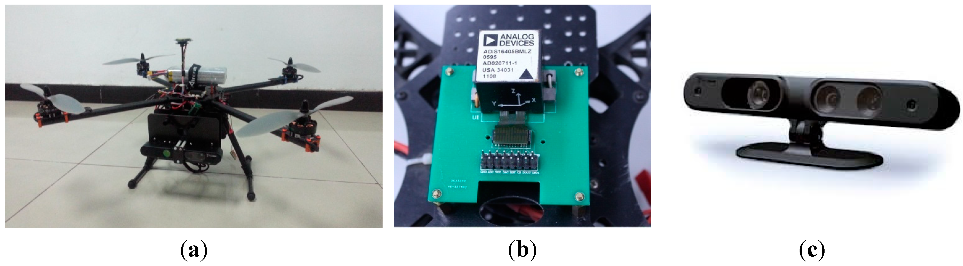
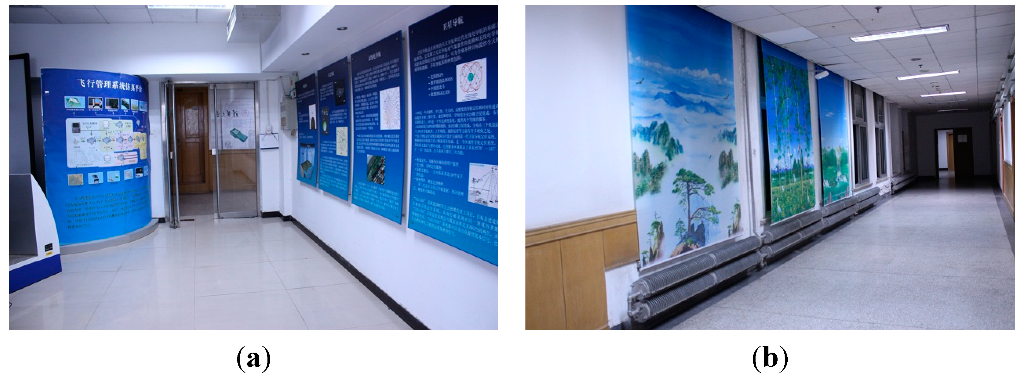
6.1. Implementation Details and Experimental Scenarios


6.2. Indoor Flight Test Results
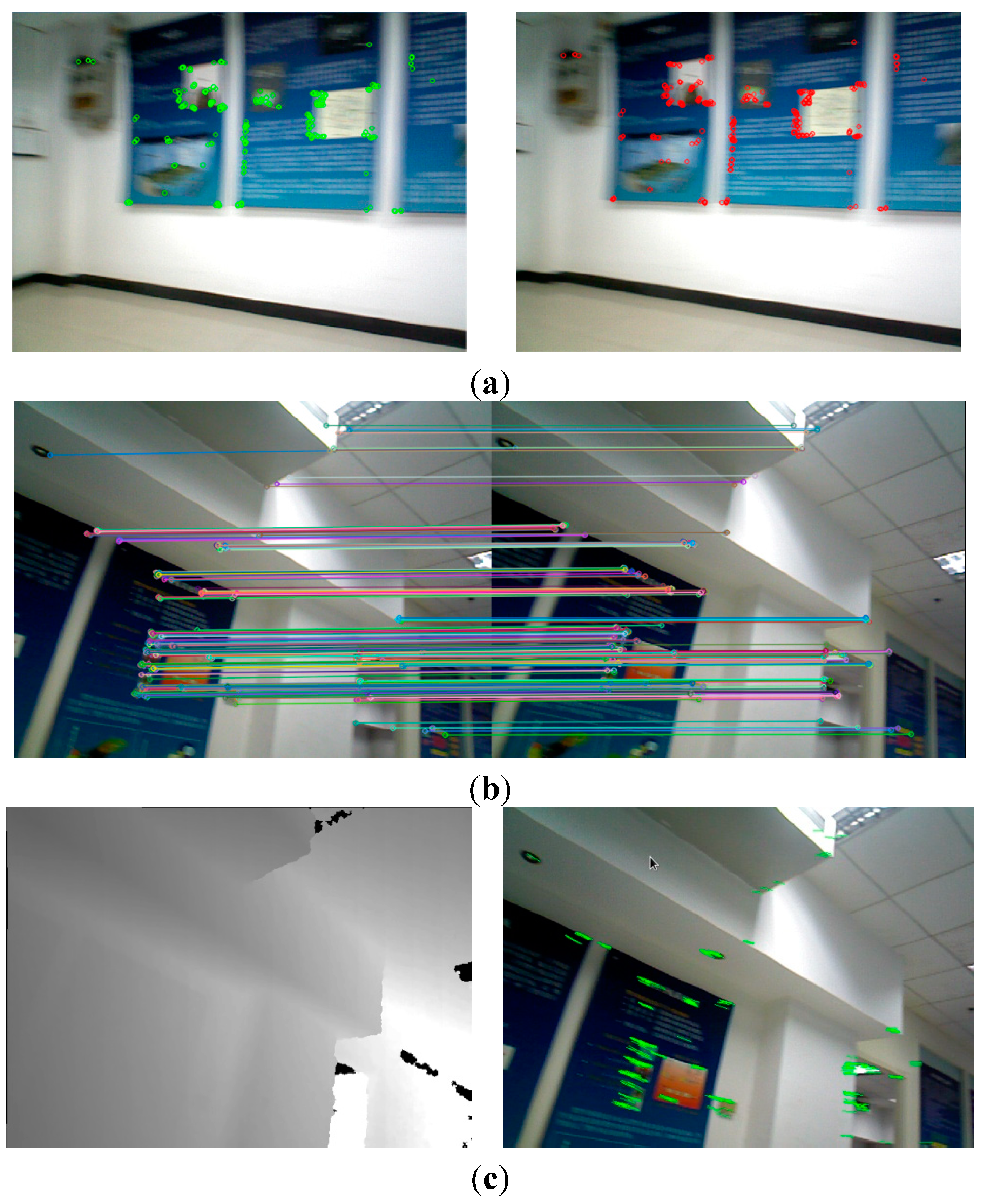
6.2.1. RGB-D Visual Odometry Test Results


| Algorithms | Average Time (ms) |
|---|---|
| Harris Corner | 16.6 |
| SIFT | 6290.1 |
| SURF | 320.5 |
| OFC-ORB | 13.2 |
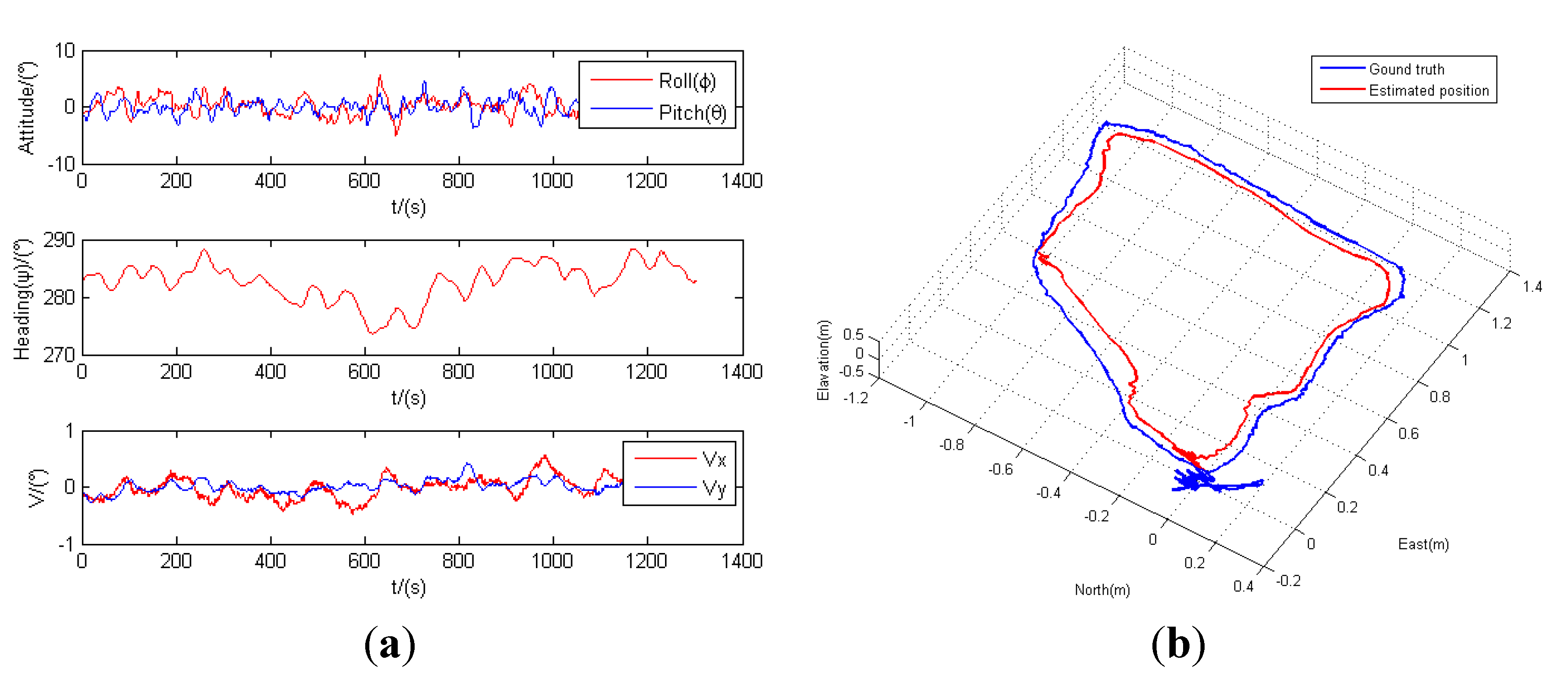
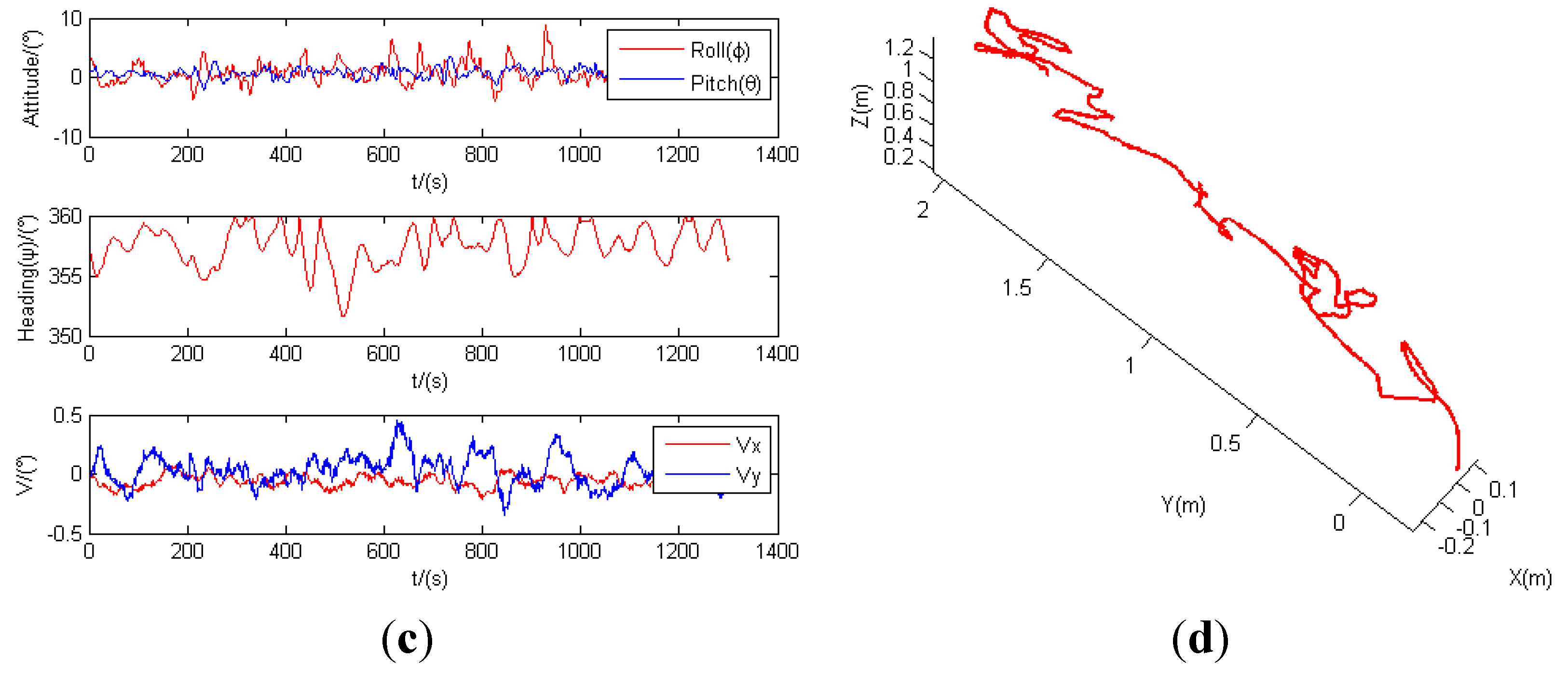
6.2.2. State Estimation Results


7. Conclusions and Future Work
Acknowledgments
Author Contributions
Conflicts of Interest
References
- Bouabdallah, S.; Bermes, C.; Grzonka, S.; Gimkiewicz, C.; Brenzikofer, A.; Hahn, R.; Schafroth, D.; Grisetti, G.; Burgard, W.; Siegwart, R. Towards palm-size autonomous helicopters. J. Intell. Robot. Syst. 2011, 61, 445–471. [Google Scholar] [CrossRef]
- Goodrich, M.A.; Cooper, J.L.; Adams, J.A.; Humphrey, C.; Zeeman, R.; Buss, B.G. Using a mini-UAV to support wilderness search and rescue: Practices for human–robot teaming. In Proceedings of 2007 IEEE International Workshop on Safety, Security and Rescue Robotics (SSRR 2007), Rome, Italy, 27–29 September 2007.
- Tomic, T.; Schmid, K.; Lutz, P.; Domel, A.; Kassecker, M.; Mair, E.; Grixa, I.L.; Ruess, F.; Suppa, M.; Burschka, D. Toward a fully autonomous UAV: Research platform for indoor and outdoor urban search and rescue. IEEE Robot. Autom. Mag. 2012, 19, 46–56. [Google Scholar] [CrossRef]
- Lin, L.; Roscheck, M.; Goodrich, M.; Morse, B. Supporting wilderness search and rescue with integrated intelligence: autonomy and information at the right time and the right place. In Proceedings of 24th AAAI Conference on Artificial Intelligence, Atlanta, GA, USA, 11–15 July 2010; pp. 1542–1547.
- Bachrach, A.; He, R.; Roy, N. Autonomous flight in unknown indoor environments. Int. J. Micro Air Veh. 2009, 4, 277–298. [Google Scholar]
- Bachrach, A.; He, R.; Roy, N. Autonomous flight in unstructured and unknown indoor environments. In Proceedings of European Conference on Micro Aerial Vehicles (EMAV 2009), Delft, The Netherlands, 14–17 September 2009.
- Bachrach, A.; Prentice, S.; He, R.; Roy, N. RANGE: Robust autonomous navigation in GPS-denied environments. J. Field Robot. 2011, 28, 644–666. [Google Scholar] [CrossRef]
- Chowdhary, G.; Sobers, D.M., Jr.; Pravitra, C.; Christmann, C.; Wu, A.; Hashimoto, H.; Ong, C.; Kalghatgi, R.; Johnson, E.N. Self-contained autonomous indoor flight with ranging sensor navigation. J. Guid. Control Dyn. 2012, 29, 1843–1854. [Google Scholar] [CrossRef]
- Chowdhary, G.; Sobers, D.M.; Pravitra, C.; Christmann, C.; Wu, A.; Hashimoto, H.; Ong, C.; Kalghatgi, R.; Johnson, E.N. Integrated guidance navigation and control for a fully autonomous indoor UAS. In Proceedings of AIAA Guidance Navigation and Control Conference, Portland, OR, USA, 8–11 August 2011.
- Sobers, D.M.; Yamaura, S.; Johnson, E.N. Laser-aided inertial navigation for self-contained autonomous indoor flight. In Proceedings of AIAA Guidance Navigation and Control Conference, Toronto, Canada, 2–5 August 2010.
- Weiss, S.; Achtelik, M.W.; Lynen, S.; Chli, M.; Siegwart, R. Real-time onboard visual-inertial state estimation and self-calibration of MAVs in unknown environments. In Proceedings of 2012 IEEE International Conference on Robotics and Automation (ICRA), Saint Paul, MN, USA, 14–18 May 2012; pp. 957–964.
- Wu, A.D.; Johnson, E.N.; Kaess, M.; Dellaert, F.; Chowdhary, G. Autonomous flight in GPS-denied environments using monocular vision and inertial sensors. J. Aerosp. Comput. Inf. Commun. 2013, 10, 172–186. [Google Scholar]
- Wu, A.D.; Johnson, E.N. Methods for localization and mapping using vision and inertial sensors. In Proceedings of AIAA Guidance, Navigation, and Control Conference, Honolulu, HI, USA, 18–21 August 2008.
- Acgtelik, M.; Bachrach, A.; He, R.; Prentice, S.; Roy, N. Stereo vision and laser odometry for autonomous helicopters in GPS-denied indoor environments. Proc. SPIE 2009, 7332, 733219. [Google Scholar]
- Achtelik, M.; Roy, N.; Bachrach, A.; He, R.; Prentice, S.; Roy, N. Autonomous navigation and exploration of a quadrotor helicopter in GPS-denied indoor environments. In Proceedings of the 1st Symposium on Indoor Flight, International Aerial Robotics Competition, Mayagüez, Puerto Rico, 21 July 2009.
- Voigt, R.; Nikolic, J.; Hurzeler, C.; Weiss, S.; Kneip, L.; Siegwart, R. Robust embedded egomotion estimation. In Proceedings of 2011 IEEE/RSJ International Conference on Intelligent Robots and Systems (IROS), San Francisco, CA, USA, 25–30 September; pp. 2694–2699.
- Bachrach, A.; Prentice, S.; He, R.; Henry, P.; Huang, A.S.; Krainin, M.; Maturana, D.; Fox, D.; Roy, N. Estimation, planning, and mapping for autonomous flight using an RGB-D camera in GPS-denied environments. Int. J. Robot. Res. 2012, 31, 1320–1343. [Google Scholar] [CrossRef]
- Leishman, R.; Macdonald, J.; McLain, T.; Beard, R. Relative navigation and control of a hexacopter. In Proceedings of 2012 IEEE International Conference on Robotics and Automation (ICRA), Saint Paul, MN, USA, 14–18 May 2012; pp. 4937–4942.
- Guerrero-Castellanos, J.F.; Madrigal-Sastre, H.; Durand, S.; Marchand, N.; Guerrero-Sanchez, W.F.; Salmeron, B.B. Design and implementation of an attitude and heading reference system (AHRS). In Proceedings of 2011 8th International Conference on Electrical Engineering Computing Science and Automatic Control (CCE), Merida, Mexico, 26–28 October 2011.
- Bonnabel, S.; Martin, P.; Salaün, E. Invariant extended Kalman filter: Theory and application to a velocity-aided attitude estimation problem. In Proceedings of Joint 48th IEEE Conference on Decision and Control and 2009 28th Chinese Control Conference (CDC/CCC 2009), Shanghai, China, 15–18 December 2009; pp. 1297–1304.
- Kelly, J.; Sukhatme, G.S. Visual-inertial sensor fusion: Localization, mapping and sensor-to-sensor self-calibration. Int. J. Robot. Res. 2011, 30, 56–79. [Google Scholar] [CrossRef]
- Van der Merwe, R.; Wan, E. Sigma-point Kalman filters for integrated navigation. In Proceedings of 60th Annual Meeting of the Institute of Navigation (ION), Dayton, OH, USA, 7–9 June 2004; pp. 641–654.
- Bry, A.; Bachrach, A.; Roy, N. State estimation for aggressive flight in GPS-denied environments using onboard sensing. In Proceedings of 2012 IEEE International Conference on Robotics and Automation (ICRA), Saint Paul, MN, USA, 14–18 May 2012; pp. 1–8.
- Crassidis, J.L.; Markley, F.L.; Cheng, Y. Survey of nonlinear attitude estimation methods. J. Guid. Control Dyn. 2007, 30, 12–28. [Google Scholar] [CrossRef]
- Achtelik, M.; Achtelik, M.; Weiss, S.; Siegwart, R. Onboard IMU and monocular vision based control for MAVs in unknown in- and outdoor environments. In Proceedings of 2011 IEEE International Conference on Robotics and Automation (ICRA), Shanghai, China, 9–13 May 2011; pp. 3056–3063.
- Boutayeb, M.; Richard, E.; Rafaralahy, H.; Souley Ali, H.; Zaloylo, G. A simple time-varying observer for speed estimation of UAV. In Proceedings of 17th IFAC World Congress, Seoul, Korea, 6–11 July 2008; pp. 1760–1765.
- Benallegue, A.; Mokhtari, A.; Fridman, L. High-order sliding-mode observer for a quadrotor UAV. Int. J. Robust Nonlinear Control 2008, 18, 427–440. [Google Scholar] [CrossRef]
- Madani, T.; Benallegue, A. Sliding mode observer and backstepping control for a quadrotor unmanned aerial vehicles. In Proceedings of 2007 American Control Conference, New York, NY, USA, 9–13 July 2007; pp. 5887–5892.
- Benzemrane, K.; Santosuosso, G.L.; Damm, G. Unmanned aerial vehicle speed estimation via nonlinear adaptive observers. In Proceedings of 2007 American Control Conference, New York, NY, USA, 9–13 July 2007.
- Rafaralahy, H.; Richard, E.; Boutayeb, M.; Zasadzinski, M. Simultaneous observer based sensor diagnosis and speed estimation of unmanned aerial vehicle. In Proceedings of 47th IEEE Conference on Decision and Control (CDC 2008), Cancun, Mexico, 9–11 December 2008; pp. 2938–2943.
- Bonnabel, S.; Martin, P.; Rouchon, P. Symmetry-preserving observers. IEEE Trans. Autom. Control 2008, 53, 2514–2526. [Google Scholar] [CrossRef]
- Bonnabel, S.; Martin, P.; Rouchon, P. Non-linear symmetry-preserving observers on lie groups. IEEE Trans. Autom. Control 2009, 54, 709–1713. [Google Scholar]
- Mahony, R.; Hamel, T.; Pflimlin, J.-M. Nonlinear complementary filters on the special orthogonal group. IEEE Trans. Autom. Control 2008, 53, 1203–1218. [Google Scholar] [CrossRef]
- Martin, P.; Salaun, E. Invariant observers for attitude and heading estimation from low-cost inertial and magnetic sensors. In Proceedings of 46th IEEE Conference on Decision and Control, New Orleans, LA, USA, 12–14 December 2007; pp. 1039–1045.
- Martin, P.; Salaun, E. Design and implementation of a low-cost attitude and heading nonlinear estimator. In Proceedings of Fifth International Conference on Informatics in Control, Automation and Robotics, Signal Processing, Systems Modeling and Control, Funchal, Portugal, 11–15 May 2008; pp. 53–61.
- Martin, P.; Salaün, E. Design and implementation of a low-cost observer-based attitude and heading reference system. Control Eng. Pract. 2010, 18, 712–722. [Google Scholar] [CrossRef]
- Bonnabel, S. Left-invariant extended Kalman filter and attitude estimation. In Proceedings of the 46th IEEE Conference on Decision and Control, New Orleans, LA, USA, 12–14 December 2007; pp. 1027–1032.
- Barczyk, M.; Lynch, A.F. Invariant extended Kalman filter design for a magnetometer-plus-GPS aided inertial navigation system. In Proceedings of the 50th IEEE Conference on Decision and Control and European Control Conference (CDC-ECC), Orlando, FL, USA, 12–15 December 2011; pp. 5389–5394.
- Barczyk, M.; Lynch, A.F. Invariant observer design for a helicopter UAV aided inertial navigation system. IEEE Trans. Control Syst. Technol. 2013, 21, 791–806. [Google Scholar] [CrossRef]
- Cheviron, T.; Hamel, T.; Mahony, R.; Baldwin, G. Robust nonlinear fusion of inertial and visual data for position, velocity and attitude estimation of UAV. In Proceedings of the 2007 IEEE International Conference on Robotics and Automation, Roma, Italy, 10–14 April 2007; pp. 2010–2016.
- Rublee, E.; Rabaud, V.; Konolige, K.; Bradski, G. ORB: An efficient alternative to SIFT or SURF. In Proceedings of the 2011 IEEE International Conference on Computer Vision (ICCV), Barcelona, Spain, 6–13 November 2011; pp. 2564–2571.
- Rosten, E.; Drummond, T. Machine learning for high-speed corner detection. In Proceedings of Computer Vision–ECCV 2006, 9th European Conference on Computer Vision, Graz, Austria, 7–13 May 2006; Springer: Berlin, Germany, 2006; Volume 1, pp. 430–443. [Google Scholar]
- Calonder, M.; Lepetit, V.; Strecha, C.; Fua, P. Brief: Binary robust independent elementary features. In Proceedings of Computer Vision–ECCV 2010, 11th European Conference on Computer Vision, Heraklion, Crete, Greece, 5–11 September 2010; Springer: Berlin, Germany; pp. 778–792.
- Lucas, B.D.; Kanade, T. An iterative image registration technique with an application to stereo vision. Proc. IJCAI 1981, 81, 674–679. [Google Scholar]
- Bouguet, J.Y. Pyramidal Implementation of the Affine Lucas Kanade Feature Tracker Description of the Algorithm. Available online: http://robots.stanford.edu/cs223b04/algo_affine_tracking.pdf (accessed on 20 April 2015).
- Arun, K.S.; Huang, T.S.; Blostein, S.D. Least-squares fitting of two 3-D point sets. IEEE Trans. Pattern Anal. Mach. Intell. 1987, 5, 698–700. [Google Scholar] [CrossRef]
- Fischler, M.A.; Bolles, R.C. Random sample consensus: A paradigm for model fitting with applications to image analysis and automated cartography. Commun. ACM 1981, 24, 381–395. [Google Scholar] [CrossRef]
- Nistér, D. Preemptive RANSAC for live structure and motion estimation. Mach. Vis. Appl. 2005, 16, 321–329. [Google Scholar] [CrossRef]
- OpenCV. Available online: http://opencv.org/ (accessed on 27 December 2014).
© 2015 by the authors; licensee MDPI, Basel, Switzerland. This article is an open access article distributed under the terms and conditions of the Creative Commons Attribution license (http://creativecommons.org/licenses/by/4.0/).
Share and Cite
Li, D.; Li, Q.; Tang, L.; Yang, S.; Cheng, N.; Song, J. Invariant Observer-Based State Estimation for Micro-Aerial Vehicles in GPS-Denied Indoor Environments Using an RGB-D Camera and MEMS Inertial Sensors. Micromachines 2015, 6, 487-522. https://doi.org/10.3390/mi6040487
Li D, Li Q, Tang L, Yang S, Cheng N, Song J. Invariant Observer-Based State Estimation for Micro-Aerial Vehicles in GPS-Denied Indoor Environments Using an RGB-D Camera and MEMS Inertial Sensors. Micromachines. 2015; 6(4):487-522. https://doi.org/10.3390/mi6040487
Chicago/Turabian StyleLi, Dachuan, Qing Li, Liangwen Tang, Sheng Yang, Nong Cheng, and Jingyan Song. 2015. "Invariant Observer-Based State Estimation for Micro-Aerial Vehicles in GPS-Denied Indoor Environments Using an RGB-D Camera and MEMS Inertial Sensors" Micromachines 6, no. 4: 487-522. https://doi.org/10.3390/mi6040487
APA StyleLi, D., Li, Q., Tang, L., Yang, S., Cheng, N., & Song, J. (2015). Invariant Observer-Based State Estimation for Micro-Aerial Vehicles in GPS-Denied Indoor Environments Using an RGB-D Camera and MEMS Inertial Sensors. Micromachines, 6(4), 487-522. https://doi.org/10.3390/mi6040487