
Low Flow Liquid Calibration Setup †

Abstract
:
1. Introduction
2. Description of the Setup and Uncertainties
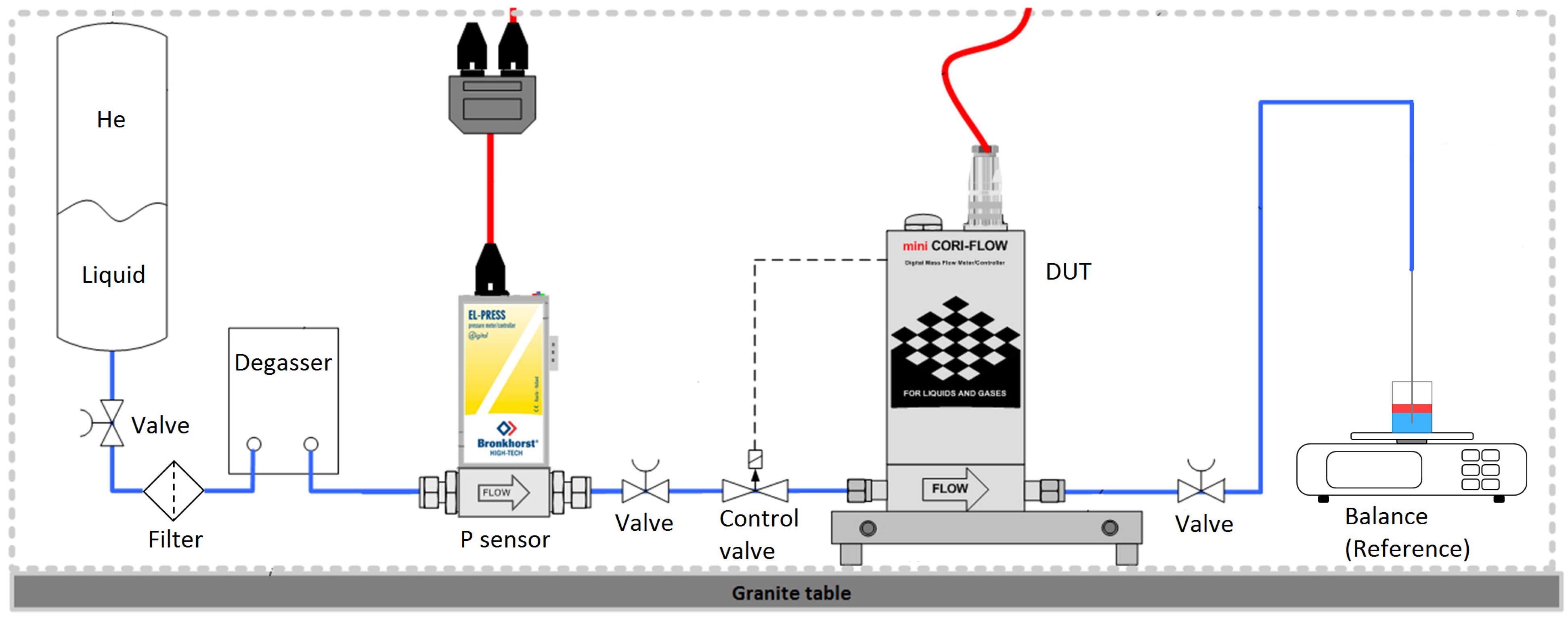
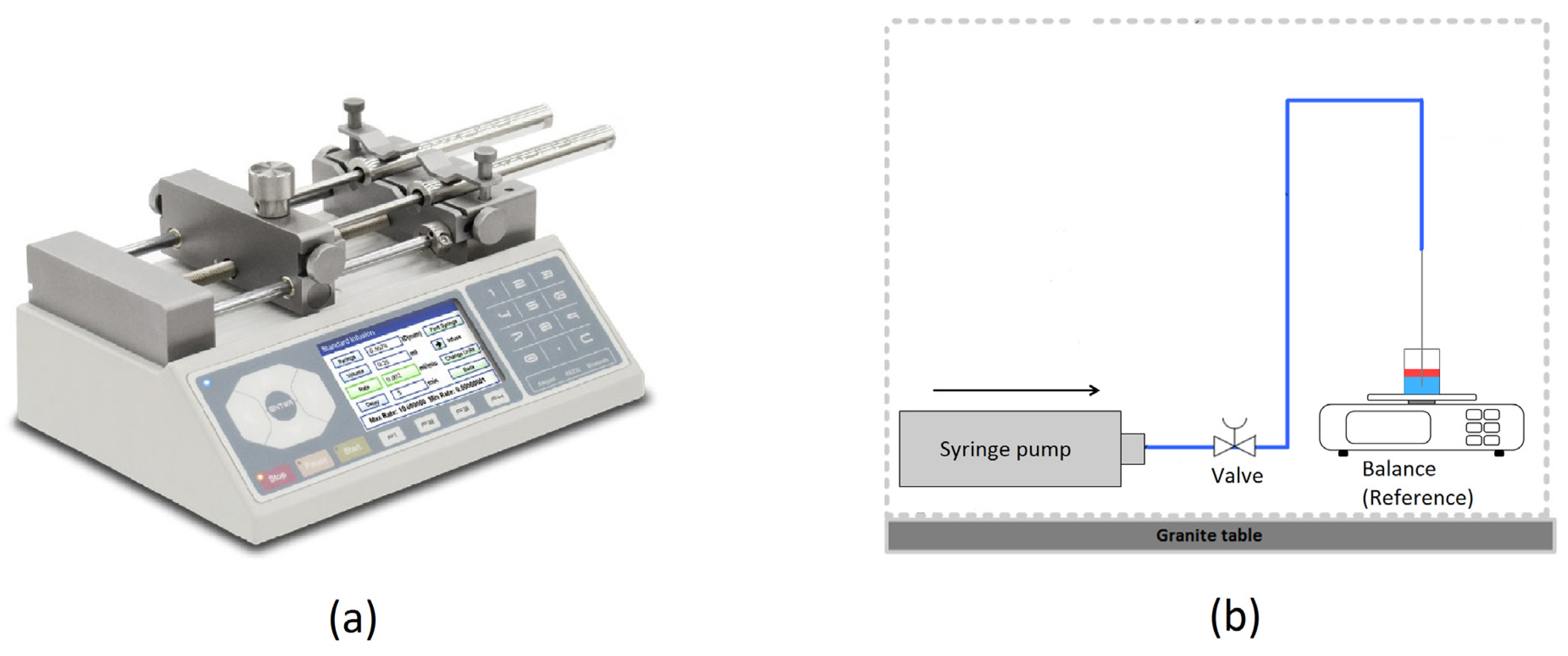
2.1. Setup
2.2. From Mass-to-Mass Flow
2.3. Description of Uncertainties
2.3.1. Mass Uncertainties
- Calibration;
- Drift;
- Readability;
- Linearity;
- Repeatability;
- Temperature sensitivity.
2.3.2. Mass Correction and Uncertainty
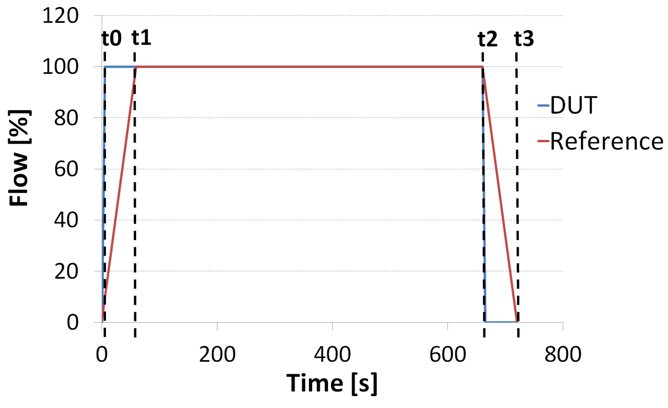
2.3.3. Time Uncertainties
2.3.4. Mass Flow Uncertainties
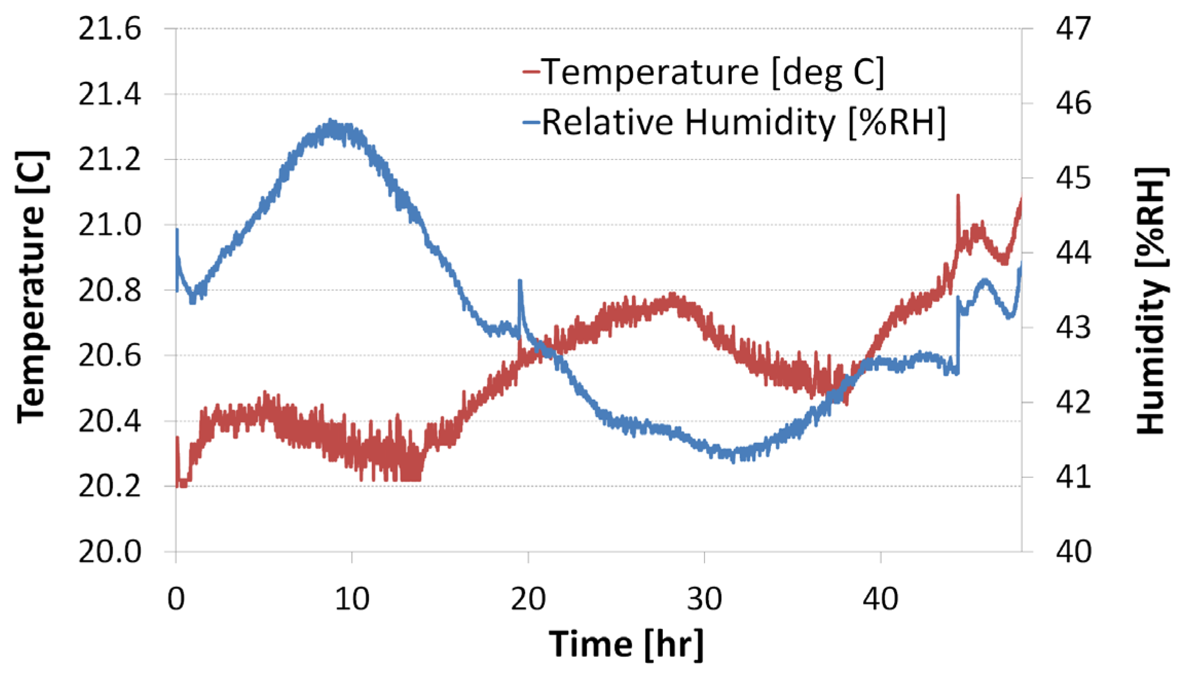
Environmental Influences


Surface Tension Effects between Tube and Fluid
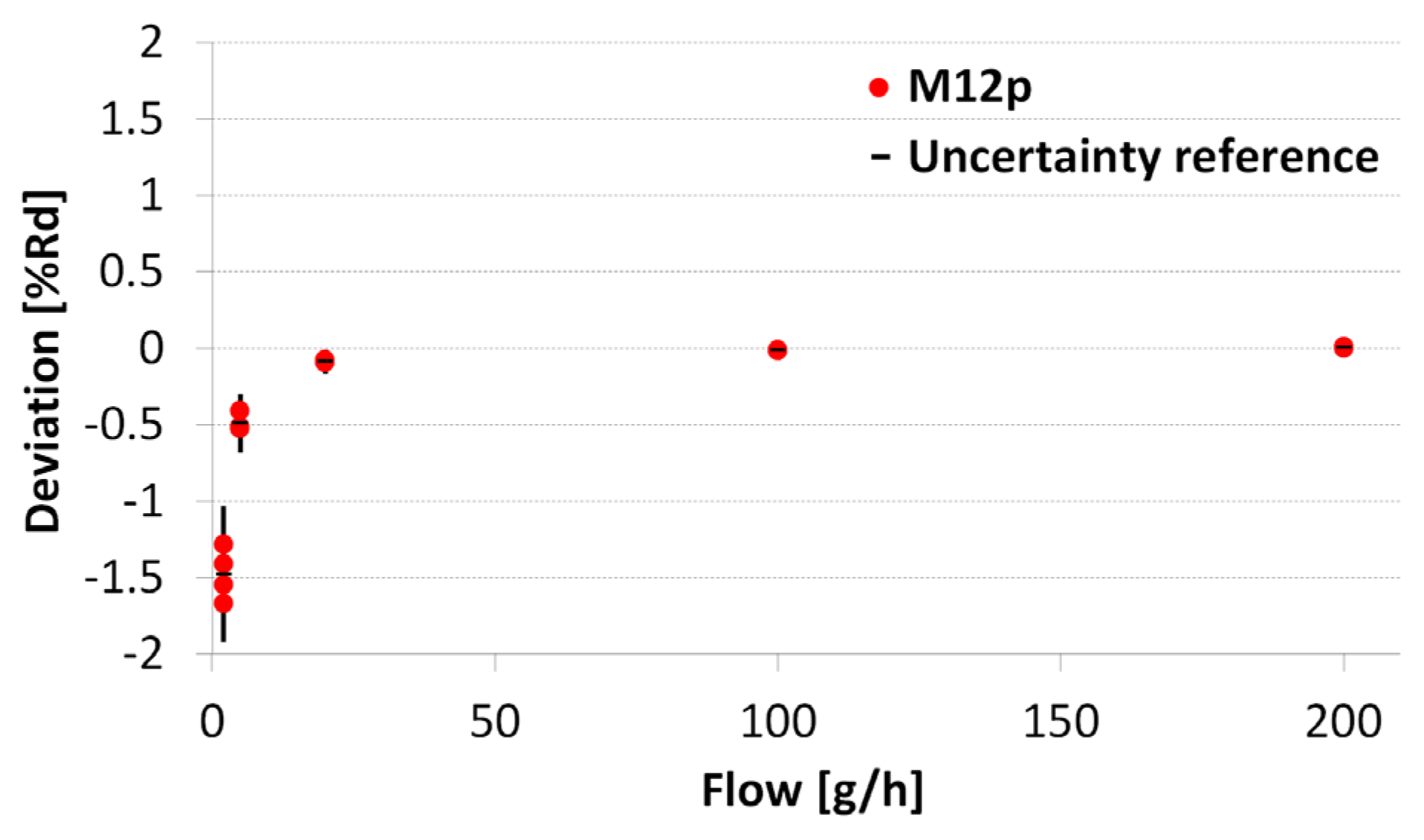
2.4. Typical Mass Flow Uncertainty
- For flow rates between 1 and 15 g/h the reference uncertainty is approximately 0.6 to 0.06%Rd (percentage of reading).
- For flow rates between 15 and 200 g/h the reference uncertainty is approximately 0.06 to 0.04%Rd.

| Component | xi value | Standard uncertainty () | Sourse number | Source name | Sensitity coeficient (ci) | Ci × | Absolute | Influence total uncertainty |
|---|---|---|---|---|---|---|---|---|
| Mr (g) | 7.50 | 4.50 × 10⁻⁶ | 1 | Scale Calibration | 2.00 | 9.01 × 10⁻⁶ | 9.01 × 10⁻⁶ | 0.08% |
| 1.55 × 10⁻⁴ | 2 | Scale_drift | 2.00 | 3.11 × 10⁻⁴ | 3.11 × 10⁻⁴ | 2.80% | ||
| 1.00 × 10⁻⁵ | 3 | Scale_readability | 2.00 | 2.00 × 10⁻⁵ | 2.00 × 10⁻⁵ | 0.18% | ||
| 1.00 × 10⁻⁴ | 4 | Scale_linearity | 2.00 | 2.00 × 10⁻⁴ | 2.00 × 10⁻⁴ | 1.80% | ||
| 1.20 × 10⁻⁴ | 5 | Scale_repeatability | 2.00 | 2.40 × 10⁻⁴ | 2.40 × 10⁻⁴ | 2.16% | ||
| 3.00 × 10⁻⁵ | 6 | Sacle_drift temperature | 2.00 | 6.01 × 10⁻⁵ | 6.01 × 10⁻⁵ | 0.54% | ||
| Mcor (g) | 7.51 | 1.88 × 10⁻⁴ | 7 | Mass-cor_rho air at calibration | 2.00 | 3.75 × 10⁻⁴ | 3.75 × 10⁻⁴ | 3.38% |
| 1.13 × 10⁻⁴ | 8 | Mass-cor_rho mass at calibration | 2.00 | 2.26 × 10⁻⁴ | 2.26 × 10⁻⁴ | 2.03% | ||
| 1.55 × 10⁻³ | 9 | Mass-cor_rho air at measurement | 2.00 | 3.10 × 10⁻³ | 3.10 × 10⁻³ | 27.92% | ||
| 5.58 × 10⁻⁴ | 10 | Mass-cor_rho object at measurement | 2.00 | 1.12 × 10⁻³ | 1.12 × 10⁻³ | 10.04% | ||
| 1.60 × 10⁻⁴ | 11 | Mass-cor_surface variation of tube | 2.00 | 3.20 × 10⁻⁴ | 3.20 × 10⁻⁴ | 2.88% | ||
| 2.10 × 10⁻⁴ | 12 | Mass-cor_surface variation of breaker | 2.00 | 4.20 × 10⁻⁴ | 4.20 × 10⁻⁴ | 3.78% | ||
| tr (s) | 1.80 × 10³ | 5.40 × 10⁻² | 13 | FBI_crystal | −8.34 × 10⁻³ | −4.50 × 10⁻⁴ | 4.50 × 10⁻⁴ | 4.05% |
| 6.19 × 10⁻² | 14 | FBI_roundings error clock | −8.34 × 10⁻³ | −5.16 × 10⁻⁴ | 5.16 × 10⁻⁴ | 4.64% | ||
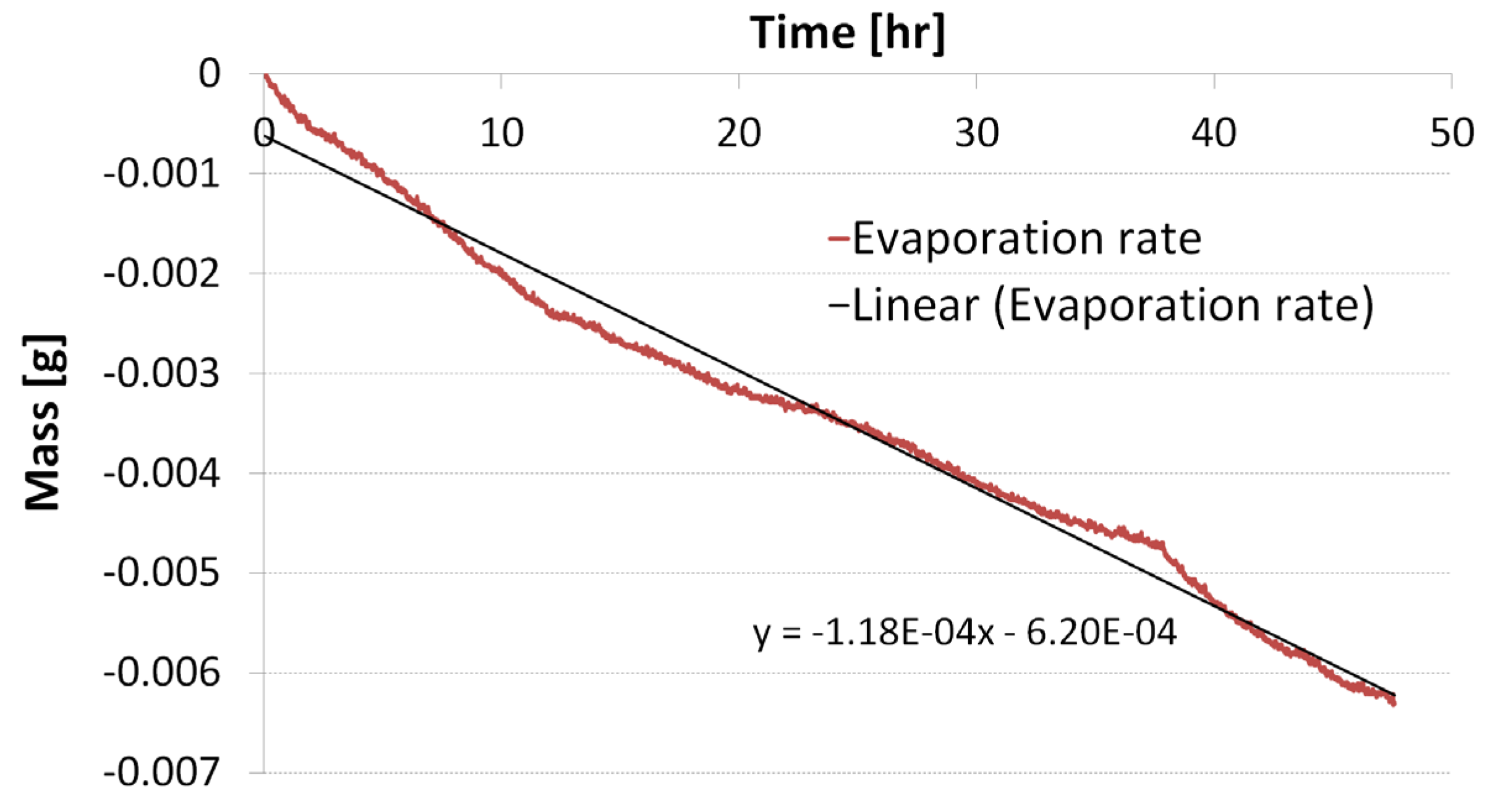
| (g/h) | 1.50 × 101 | 3.54 × 10⁻⁴ | 15 | Massflow_evaporation rate | 1.00 | 3.54 × 10⁻⁴ | 3.54 × 10⁻⁴ | 3.19% |
| 3.00 × 10⁻³ | 16 | Massflow_surfacetension/sticky | 1.00 | 3.00 × 10⁻³ | 3.00 × 10⁻³ | 27.00% | ||
| 3.93 × 10⁻⁴ | 17 | Massflow_volume expansion medium | 1.00 | 3.93 × 10⁻⁴ | 3.93 × 10⁻⁴ | 3.54% | ||
| (g/h) | 1.50 × 101 | u() (g/h) | 9.23 × 10⁻³ | 100% | ||||
| u() (%) | 0.06% |
3. Experimental Section
3.1. Procedures
3.1.1. Pure Liquid
3.1.2. Stable Mass Flow
3.1.3. Calibration
3.2. Measurements
3.2.1. Mass Flow Meter as Flow Controller
3.2.2. Syringe Pump as Flow Generator
3.2.3. Intercomparison
4. Results
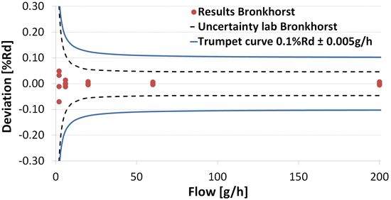
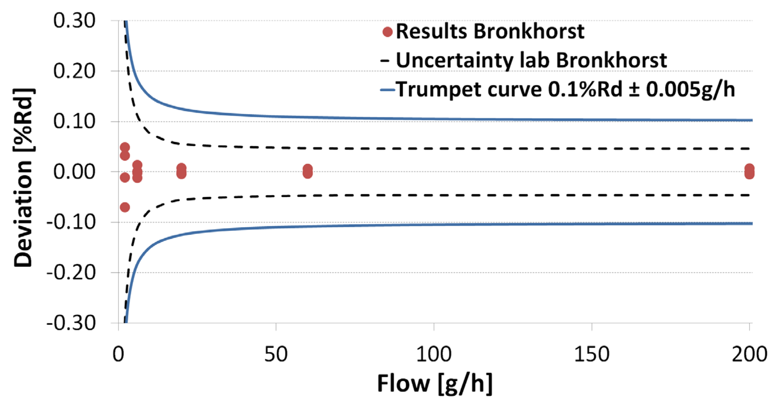
4.1. Mass Flow Meter
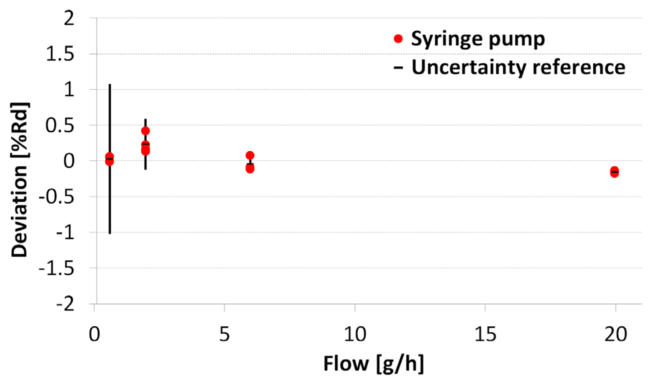
4.2. Syringe Pump

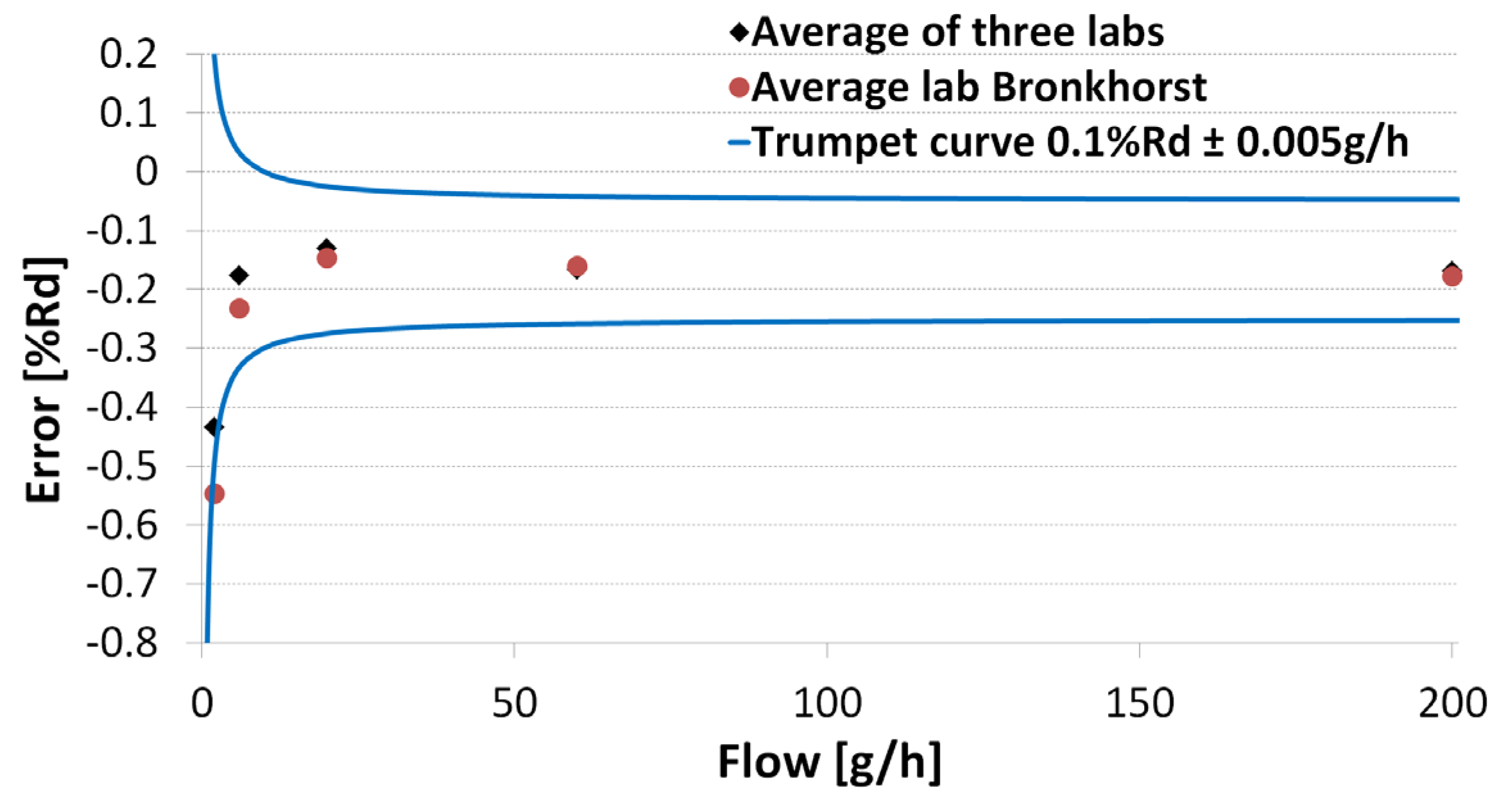
4.3. Intercomparison

| Bronkhorst results | Uncertainty setup (%) | En value (-) | |
|---|---|---|---|
| Flow rate (g/h) | Error (%) | ||
| 2 | −0.55 | 0.31 | 0.05 |
| 6 | −0.23 | 0.11 | 0.21 |
| 20 | −0.14 | 0.06 | 0.05 |
| 60 | −0.16 | 0.06 | 0.10 |
| 200 | −0.17 | 0.10 | 0.14 |
5. Conclusions
Acknowledgments
Author Contributions
Conflicts of Interest
References
- Metrology for Drug Delivery, EU-Funded Research Project 2012–2015. Available online: http://www.drugmetrology.com/ (accessed on 16 April 2015).
- Fox, R.W.; McDonald, A.T.; Pritchard, P.J. Introduction to Fluid Mechanics, 6th ed.; John Wiley and Sons: Chichester, NY, USA, 2004. [Google Scholar]
- Shinder, I.I.; Marfenko, I.V. NIST Calibration Services for Water Flowmeters: Water Flow Calibration Facility; NIST Special Publication 250; National Institute of Standards and Technology (NIST): Gaithersburg, MD, USA, 2006. [Google Scholar]
- Lucas, P. MeDD - Task 1.1. Intercomparison Supplement Report. May 2014. Available online: http://www.drugmetrology.com/images/2014.07.30_MeDD_-_comparison_supplement_report.pdf (accessed on 30 July 2014).
- David, C. MeDD - Task 1.1. Intercomparison Report. December 2013. Available online: http://www.drugmetrology.com/images/Publications/2014.07.30_MeDD_-_comparison_report.pdf (accessed on 30 July 2014).
© 2015 by the authors; licensee MDPI, Basel, Switzerland. This article is an open access article distributed under the terms and conditions of the Creative Commons Attribution license (http://creativecommons.org/licenses/by/4.0/).
Share and Cite
Platenkamp, T.H.; Sparreboom, W.; Ratering, G.H.J.M.; Katerberg, M.R.; Lötters, J. Low Flow Liquid Calibration Setup. Micromachines 2015, 6, 473-486. https://doi.org/10.3390/mi6040473
Platenkamp TH, Sparreboom W, Ratering GHJM, Katerberg MR, Lötters J. Low Flow Liquid Calibration Setup. Micromachines. 2015; 6(4):473-486. https://doi.org/10.3390/mi6040473
Chicago/Turabian StylePlatenkamp, Tom H., Wouter Sparreboom, Gijs H. J. M. Ratering, Marcel R. Katerberg, and Joost Lötters. 2015. "Low Flow Liquid Calibration Setup" Micromachines 6, no. 4: 473-486. https://doi.org/10.3390/mi6040473
APA StylePlatenkamp, T. H., Sparreboom, W., Ratering, G. H. J. M., Katerberg, M. R., & Lötters, J. (2015). Low Flow Liquid Calibration Setup. Micromachines, 6(4), 473-486. https://doi.org/10.3390/mi6040473