
Adaptive Covariance Estimation Method for LiDAR-Aided Multi-Sensor Integrated Navigation Systems


Abstract
:1. Introduction
2. Related Work
- (1)
- The first step is preprocessing, which is an optional procedure on the LiDAR measurements. In [10,21], a median filter is used to filter out some of the outliers and noises, while a six order polynomial fitting is used in [22,23] between the measured distance and the true distance to compensate for the systematic error.
- (2)
- The following step is to segment scan points into different groups, each of which includes points belonging to the same line. Generally, there are three segmentation or breakpoint detection methods: one is based on the Euclidean distance between two consecutive scanned points, while the others are KF-based segmentation methods and the fuzzy cluster method [23,24,25].
- (3)
- Then, the line parameters are computed. The most commonly used line fitting techniques are the Hough transform (HT) [26] and least squares. HT can be used to extract line features by transforming the image pixel into the parameter space and detecting peaks in that space. However, HT has some drawbacks, like the occurrence of multi-peaks due to the discretization of the image and the parameter space, as indicated in [27].
- (4)
- Finally, collinear lines are merged into one line feature making the process more efficient.
- (1)
- The covariance of LiDAR-derived relative pose change is estimated. This is crucial when the LiDAR-derived relative pose changes are to be fused with information from other sensors. The proposed adaptive covariance estimation method can be applied in any LiDAR-based integrated navigation system.
- (2)
- The LiDAR intensity measurements are used to weight the influence of each scanned point on the line parameters estimation.
- (3)
- The influences of the geometric layout of the environment (especially the long corridor) and line feature extraction error are addressed.
3. Line Extraction Method
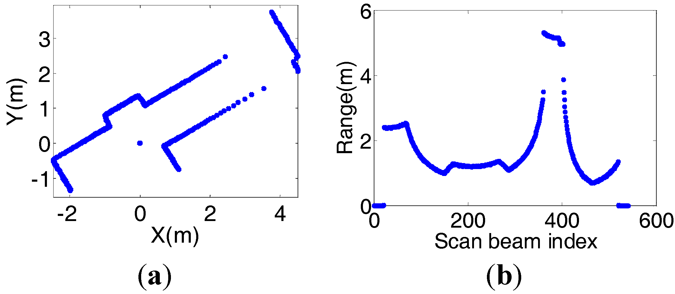
3.1. Segmentation
3.1.1. Breakpoint Detection
3.1.2. Corner Detection

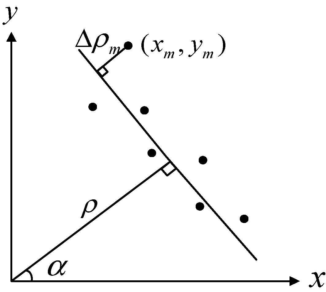
3.2. Line Parameters Calculation

3.2.1. Scan Points’ Weight Calculation
3.2.2. Line Parameters Estimation
3.2.3. Line Quality Calculation
3.3. Line Merging
3.4. Pose Change and Covariance Estimation
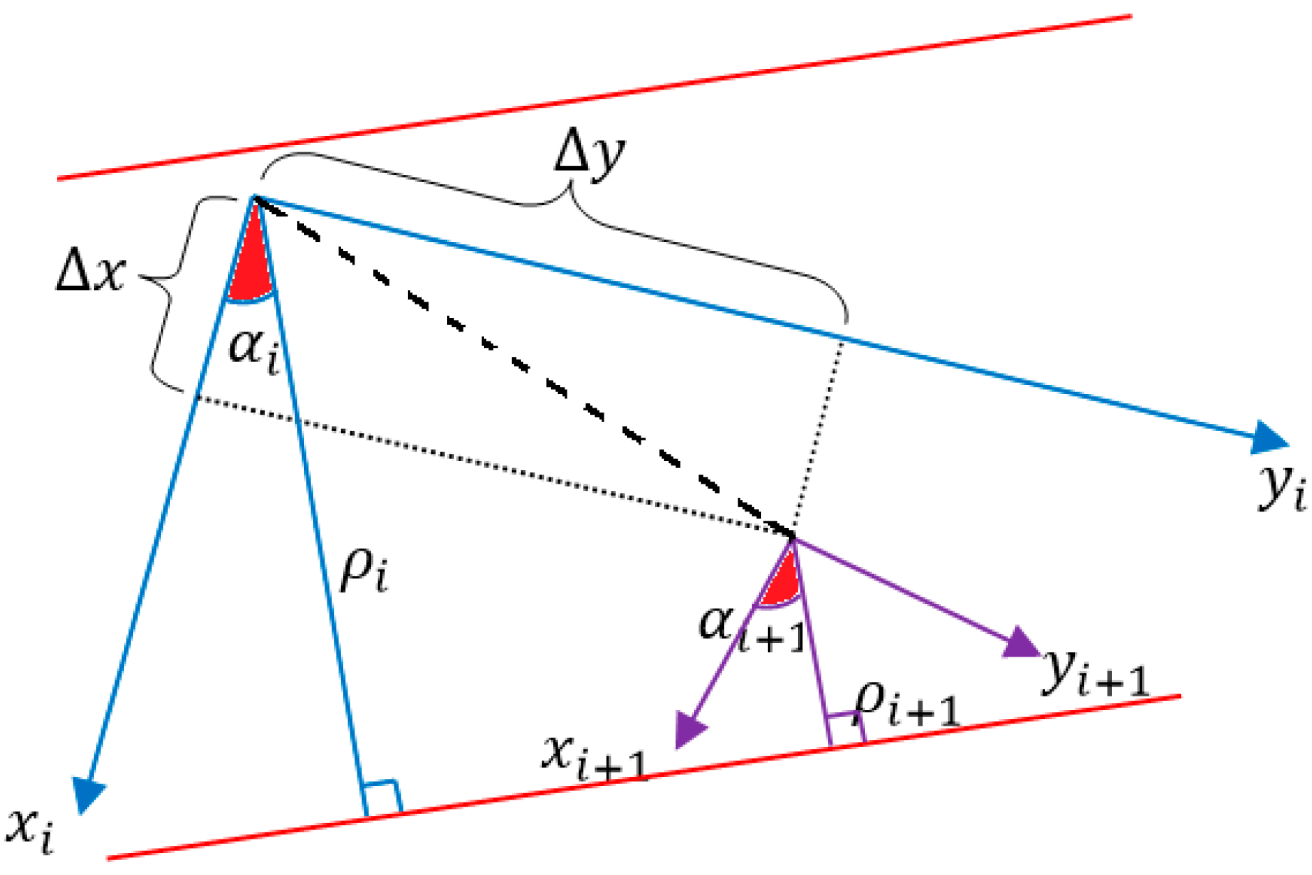
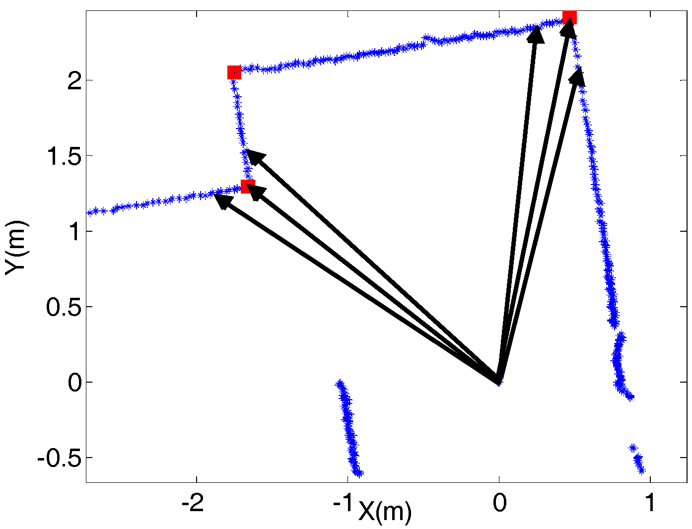
3.4.1. Position Change and Covariance Estimation
3.4.2. Azimuth Change and Covariance Estimation
3.4.3. Singularity Issue
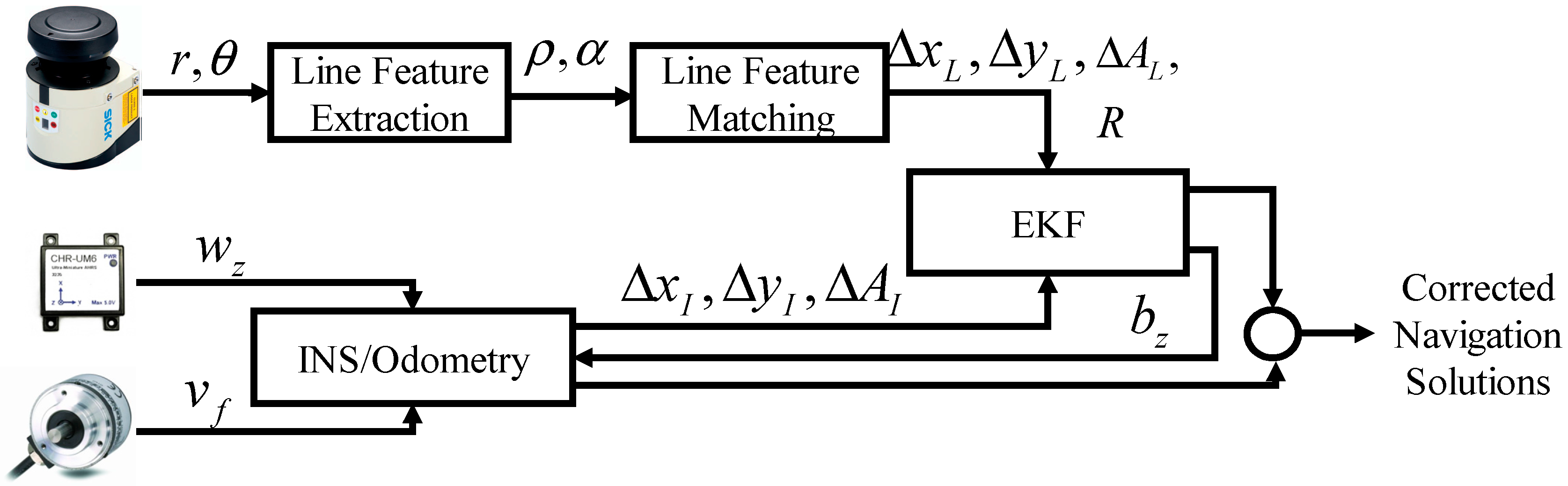
4. The Integrated Solution and Filter Design

4.1. System Model
4.2. Measurement Model
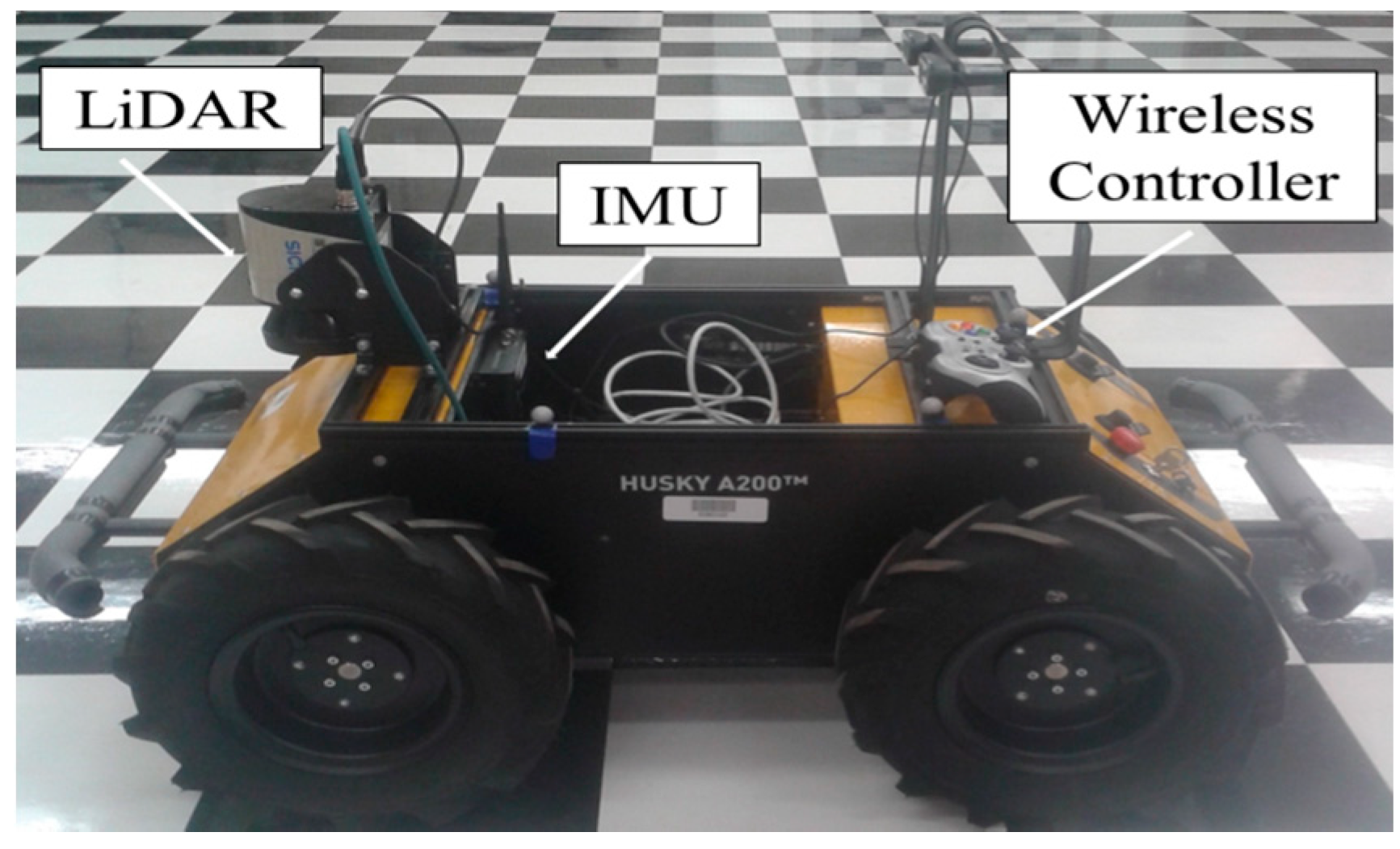
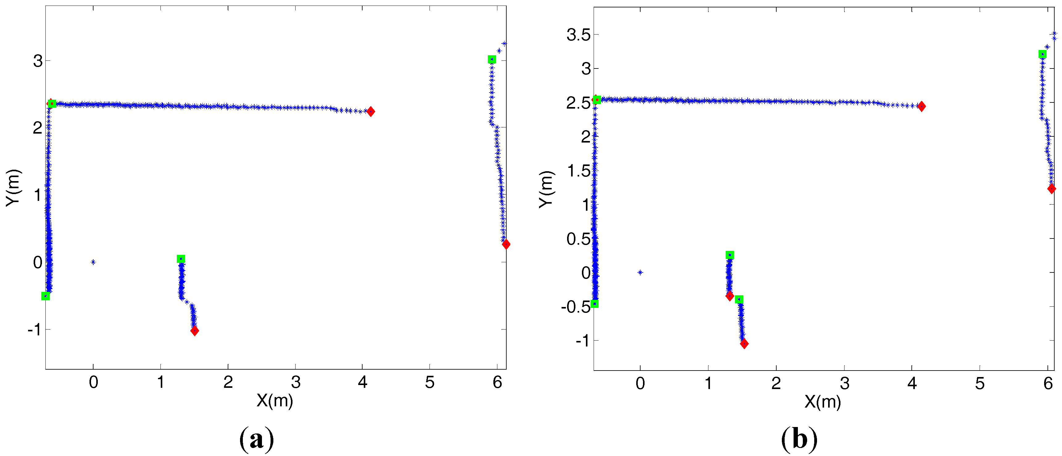
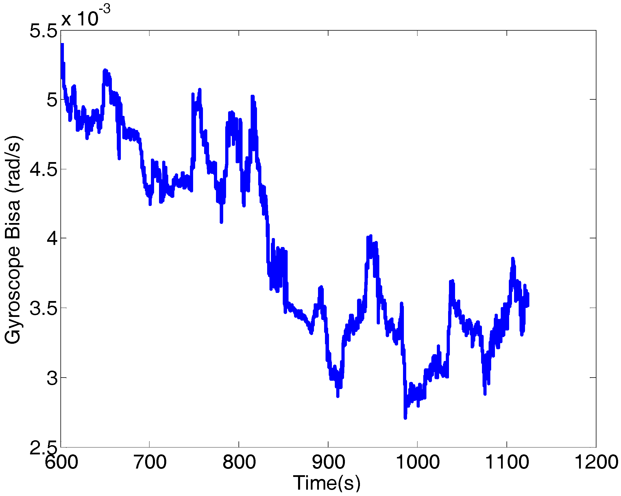
5. Experiment Results and Analysis


| Parameter | Value |
|---|---|
| Statistical Error (mm) | ±12 |
| Angular Resolution (°) | 0.5 |
| Maximum Measurement Range (m) | 20 |
| Scanning Range (°) | 270 |
| Scanning Frequency (Hz) | 50 |

| Example | Δx (m) | Δy (m) | Cov (Δx) | Cov (Δy) |
|---|---|---|---|---|
| Example 1 | 0.3801 | 30.1185 | 0.0041 | 20.6805 |
| Example 2 | 0.0602 | 0.2057 | 0.0001025 | 0.0001956 |

6. Conclusions
Author Contributions
Conflicts of Interest
References
- Gutmann, J.-S.; Schlegel, C. Amos: Comparison of scan matching approaches for self-localization in indoor environments. In Proceedings of the First Euromicro Workshop on Advanced Mobile Robot, Kaiserslautern, Germany, 9–11 October 1996; pp. 61–67.
- Hesch, J.A.; Mirzaei, F.M.; Mariottini, G.L.; Roumeliotis, S.I. A laser-aided inertial naviagtion system (L-INS) for human localization in unknown indoor environments. In Proceedings of the 2010 IEEE International Conference on Robotics and Automation (ICRA), Anchorage, AK, USA, 3–7 May 2010.
- Kohlbrecher, S.; Von Stryk, O.; Meyer, J.; Klingauf, U. A flexible and scalable slam system with full 3D motion estimation. In Proceedings of the 2011 IEEE International Symposium on Safety, Security, and Rescue Robotics (SSRR), 1–5 November 2011; pp. 155–160.
- Boehler, W.; Bordas Vicent, M.; Marbs, A. Investigating laser scanner accuracy. Int. Arch. Photogramm. Remote Sens. Spat. Inf. Sci. 2003, 34, 696–701. [Google Scholar]
- Martínez, J.L.; González, J.; Morales, J.; Mandow, A.; García-Cerezo, A.J. Mobile robot motion estimation by 2D scan matching with genetic and iterative closest point algorithms. J. Field Robot. 2006, 23, 21–34. [Google Scholar] [CrossRef]
- Garulli, A.; Giannitrapani, A.; Rossi, A.; Vicino, A. Mobile robot SLAM for line-based environment representation. In Proceedings of the 44th IEEE Conference on Decision and Control,2005 and 2005 European Control Conference (CDC-ECC'05), Seville, Spain, 12–15 December 2005; pp. 2041–2046.
- Arras, K.O.; Siegwart, R.Y. Feature Extraction and Scene Interpretation for Map-Based Navigation and Map Building; Intelligent Systems & Advanced Manufacturing, International Society for Optics and Photonics: Pittsburgh, PA, USA, 1998; pp. 42–53. [Google Scholar]
- Soloviev, A.; Bates, D.; van Graas, F. Tight coupling of laser scanner and inertial measurements for a fully autonomous relative navigation solution. Navigation 2007, 54, 189–205. [Google Scholar] [CrossRef]
- Pfister, S.T.; Roumeliotis, S.I.; Burdick, J.W. Weighted line fitting algorithms for mobile robot map building and efficient data representation. In Proceedings of the IEEE International Conference on Robotics and Automation (2003ICRA'03), 14–19 September 2003; pp. 1304–1311.
- Lingemann, K.; Nüchter, A.; Hertzberg, J.; Surmann, H. High-speed laser localization for mobile robots. Robot. Auton. Syst. 2005, 51, 275–296. [Google Scholar] [CrossRef]
- Aghamohammadi, A.A.; Taghirad, H.D.; Tamjidi, A.H.; Mihankhah, E. Feature-based range scan matching for accurate and high speed mobile robot localization. In Proceedings of the 3rd European Conference on Mobile Robots, Freiburg, Germany, 19–21 September 2007.
- Kammel, S.; Pitzer, B. Lidar-based lane marker detection and mapping. In Proceedings of the 2008 IEEE Intelligent Vehicles Symposium, Eindhoven, The Netherlands, 4–6 June 2008; pp. 1137–1142.
- Núñez, P.; Vazquez-Martin, R.; Bandera, A.; Sandoval, F. Fast laser scan matching approach based on adaptive curvature estimation for mobile robots. Robotica 2009, 27, 469–479. [Google Scholar] [CrossRef]
- Shen, S.; Michael, N.; Kumar, V. Autonomous multi-floor indoor navigation with a computationally constrained MAV. In Proceedings of the 2011 IEEE International Conference on Robotics and automation (ICRA), Shanghai, China, 9–13 May 2011; pp. 20–25.
- Segal, A.; Haehnel, D.; Thrun, S. Generalized-ICP. In Proceedings of the Robotics: Science and Systems 2009 Conference, University of Washington, Seattle, WA, USA, 28 June–1 July 2009.
- Censi, A. An ICP variant using a point-to-line metric. In Proceedings of the 2008 IEEE International Conference on Robotics and Automation (ICRA 2008), Pasadena, CA, USA, 19–23 May 2008; pp. 19–25.
- Weiß, G.; Puttkamer, E. A map based on laserscans without geometric interpretation. Intell. Auton. Syst. 1995, 4, 403–407. [Google Scholar]
- Censi, A.; Iocchi, L.; Grisetti, G. Scan matching in the Hough domain. In Proceedings of the 2005 IEEE International Conference on Robotics and Automation (ICRA 2005), Barcelona, Spain, 18–22 April 2005; pp. 2739–2744.
- Burguera, A.; González, Y.; Oliver, G. On the use of likelihood fields to perform sonar scan matching localization. Auton. Robot. 2009, 26, 203–222. [Google Scholar] [CrossRef]
- Olson, E.B. Real-time correlative scan matching. In Proceedings of the IEEE International Conference on Robotics and Automation (ICRA'09), Kobe, Japan, 12–17 May 2009; pp. 4387–4393.
- Diosi, A.; Kleeman, L. Laser scan matching in polar coordinates with application to SLAM. In Proceedings of the 2005 IEEE/RSJ International Conference on Intelligent Robots and Systems (IROS 2005), Edmonton, AB, Canada, 2–6 August 2005; pp. 3317–3322.
- Núñez, P.; Vázquez-Martín, R.; Del Toro, J.; Bandera, A.; Sandoval, F. Natural landmark extraction for mobile robot navigation based on an adaptive curvature estimation. Robot. Auton. Syst. 2008, 56, 247–264. [Google Scholar] [CrossRef]
- Borges, G.A.; Aldon, M.-J. Line extraction in 2D range images for mobile robotics. J. Intell. Robot. Syst. 2004, 40, 267–297. [Google Scholar] [CrossRef]
- Premebida, C.; Nunes, U. Segmentation and geometric primitives extraction from 2D laser range data for mobile robot applications. Robotica 2005, 2005, 17–25. [Google Scholar]
- Xia, Y.; Chun-Xia, Z.; Min, T.Z. Lidar scan-matching for mobile robot localization. Inf. Technol. J. 2010, 9, 27–33. [Google Scholar] [CrossRef]
- Ji, J.; Chen, G.; Sun, L. A novel hough transform method for line detection by enhancing accumulator array. Pattern Recognit. Lett. 2011, 32, 1503–1510. [Google Scholar] [CrossRef]
- Fernandes, L.A.; Oliveira, M.M. Real-time line detection through an improved hough transform voting scheme. Pattern Recognit. 2008, 41, 299–314. [Google Scholar] [CrossRef]
- Nguyen, V.; Martinelli, A.; Tomatis, N.; Siegwart, R. A comparison of line extraction algorithms using 2D laser rangefinder for indoor mobile robotics. In Proceedings of the 2005 IEEE/RSJ International Conference on Intelligent Robots and Systems (IROS 2005), Edmonton, AB, Canada, 2–6 August 2005; pp. 1929–1934.
- Diosi, A.; Kleeman, L. Uncertainty of line segments extracted from static SICK PLS laser scans, SICK PLS laser. In Proceedings of the Australiasian Conference on Robotics and Automation, Brisbane, Australia, 1–3 December 2003.
- Soloviev, A. Tight coupling of GPS and INS for urban navigation. Aerosp. Electron. Syst. IEEE Trans. 2010, 46, 1731–1746. [Google Scholar] [CrossRef]
- Hancock, J.; Hebert, M.; Thorpe, C. Laser intensity-based obstacle detection. In Proceedings of the 1998 IEEE/RSJ International Conference on Intelligent Robots and Systems, Victoria, BC, USA, 13–17 October 1998; pp. 1541–1546.
- Iqbal, U.; Okou, A.F.; Noureldin, A. An integrated reduced inertial sensor system—RISS/GPS for land vehicle. In Proceedings of the Position, Location and Navigation Symposium, 2008 IEEE/ION, Monterey, CA, USA, 5–8 May 2008; pp. 1014–1021.
- Iqbal, U.; Karamat, T.B.; Okou, A.F.; Noureldin, A. Experimental results on an integrated GPS and multisensor system for land vehicle positioning. Int. J. Navig. Obs. 2009, 2009, 765010. [Google Scholar]
- Liu, S.; Atia, M.M.; Karamat, T.; Givigi, S.; Noureldin, A. A dual-rate multi-filter algorithm for LiDAR-aided indoor navigation systems. In Proceedings of the Position, Location and Navigation Symposium-PLANS 2014, 2014 IEEE/ION, Monterey, CA, USA, 5–8 May 2014; pp. 1014–1019.
- Liu, S.; Atia, M.M.; Karamat, T.B.; Noureldin, A. A LiDAR-aided indoor navigation system for UGVs. J. Navig. 2014. [Google Scholar] [CrossRef]
- CHRobotics. UM6 ultra-miniature orientation sensor datasheet. Available online: http://www.chrobotics.com/docs/UM6_datasheet.pdf (accessed on 21 January 2015).
- SICK. Operating Instructions: LMS100/111/120 Laser Measurement Systems; SICK AG: Waldkirch, Germany, 2008. [Google Scholar]
© 2015 by the authors; licensee MDPI, Basel, Switzerland. This article is an open access article distributed under the terms and conditions of the Creative Commons Attribution license (http://creativecommons.org/licenses/by/4.0/).
Share and Cite
Liu, S.; Atia, M.M.; Gao, Y.; Noureldin, A. Adaptive Covariance Estimation Method for LiDAR-Aided Multi-Sensor Integrated Navigation Systems. Micromachines 2015, 6, 196-215. https://doi.org/10.3390/mi6020196
Liu S, Atia MM, Gao Y, Noureldin A. Adaptive Covariance Estimation Method for LiDAR-Aided Multi-Sensor Integrated Navigation Systems. Micromachines. 2015; 6(2):196-215. https://doi.org/10.3390/mi6020196
Chicago/Turabian StyleLiu, Shifei, Mohamed Maher Atia, Yanbin Gao, and Aboelmagd Noureldin. 2015. "Adaptive Covariance Estimation Method for LiDAR-Aided Multi-Sensor Integrated Navigation Systems" Micromachines 6, no. 2: 196-215. https://doi.org/10.3390/mi6020196
APA StyleLiu, S., Atia, M. M., Gao, Y., & Noureldin, A. (2015). Adaptive Covariance Estimation Method for LiDAR-Aided Multi-Sensor Integrated Navigation Systems. Micromachines, 6(2), 196-215. https://doi.org/10.3390/mi6020196