Calibration of Nanopositioning Stages

Abstract

Accuracy is one of the most important criteria for the performance evaluation of micro- and nanorobots or systems. Nanopositioning stages are used to achieve the high positioning resolution and accuracy for a wide and growing scope of applications. However, their positioning accuracy and repeatability are not well known and difficult to guarantee, which induces many drawbacks for many applications. For example, in the mechanical characterisation of biological samples, it is difficult to perform several cycles in a repeatable way so as not to induce negative influences on the study. It also prevents one from controlling accurately a tool with respect to a sample without adding additional sensors for closed loop control. This paper aims at quantifying the positioning repeatability and accuracy based on the ISO 9283:1998 standard, and analyzing factors influencing positioning accuracy onto a case study of 1-DoF (Degree-of-Freedom) nanopositioning stage. The influence of thermal drift is notably quantified. Performances improvement of the nanopositioning stage are then investigated through robot calibration (i.e., open-loop approach). Two models (static and adaptive models) are proposed to compensate for both geometric errors and thermal drift. Validation experiments are conducted over a long period (several days) showing that the accuracy of the stage is improved from typical micrometer range to 400 nm using the static model and even down to 100 nm using the adaptive model. In addition, we extend the 1-DoF calibration to multi-DoF with a case study of a 2-DoF nanopositioning robot. Results demonstrate that the model efficiently improved the 2D accuracy from 1400 nm to 200 nm.

1. Introduction

Nanopositioning stages are used for a wide and growing scope of applications at the microscale, such as micromanipulation, MEMS (Micro-Electro-Mechanical-Systems), mini-invasive surgery, biological and biomedical characterization [1,2,3,4]. Most of these applications require one to control very accurately the relative position and/or trajectories between a sample (for example, component to handle, tissue or living cell) and a tool used for manipulation or characterization purposes. In most cases, this ability directly and strongly impacts the results such as the success rate and resolution of the characterization or analysis [5].

Because of their capability to generate high-resolution motions, nanopositioning stages are usually used to build the micro-nanopositioning robots. Based on the compliant principle, such stages are designed with active-material-based actuators that are able to generate translation and frictionless motions. The compliant structure is also capable of amplifying the actuators’ movement. Such mechanisms are popular for microscale applications since they prevent from any mechanical drawbacks such as backlash and/or friction usually met in micropositioning stages with ballscrew bearings [6]. The compliant mechanisms generally generate a small range of motion (smaller than 500 μm) but very high resolution (in the nanometer range), straightness, and flatness [7,8,9,10], which make nanopositioning stages a key technology for applications requiring a high positioning accuracy. However, despite the widespread use, high potential, and strong efforts done to design and fabricate new nanopositioning stages, several negative specificities still have to be overcome to reach the desired performances:

• Actuators have nonlinear and sometimes time-varying behaviors, e.g., hysteresis and creep [11].
• The mechanical structure is influenced by environmental conditions. For example, the thermal expansion of a 5 cm long aluminium bar (typical size of nanopositioning stages) subjected to 1 ${}^{\circ }$C change (typical change that may happen in a controlled environment) may reach 1.2 μm which is roughly 1000 times the stage’s resolution.
• Sensors integrated (if any) in the stage suffer from extremely complex trade-off because many conditions must be met at the same time, such as small volumes, nanometer resolutions, motion ranges of several hundred micrometers, and high bandwidths. To partially tackle this limitation, integrated sensors usually measure the local motion generated by the actuator in front of the compliant structure or at a location of the compliant structure with a maximum mechanical strain (i.e., in the compliant joints). This indirect measurement technique (meaning that the output motion of the stage is not measured directly) requires a model to estimate the motion of the stage. In spite of using the efficient closed-loop control, the problem of locating accurately the mobile-part output of the stage remains.

In addition to these difficulties, achieving the aforementioned micro-nano tasks usually requires control of the nanopositioning stage and position the end-effector with respect to a fixed reference frame; for instance, to insert a needle into a cell with respect to the microscope frame. On one hand, additional sensors may be used to provide an outer-loop control (the often used inner-loop feedback one is based on internal sensors of the stages) [12]. However, a key limitation is the complexity of integrating sensors able to measure a relative position with required range, resolution, bandwidth and number of DoF (Degree-of-Freedom) [13]. For example, dedicated machines used for microsystems fabrication enable to position a component relative to the others in the plane with an accuracy of a few tens of nanometers. Nevertheless, they are usually designed for single purposes and extremely costly (in the millions of euros range). On the other hand, it is possible to control nanopositioning stages in open loop at the task level while keeping the inner loop based on internal nanopositioning stage sensors [14,15,16]. The open loop method can be realized with the calibration approach [17,18,19] where a good and reliable model is required to depict the whole system inclusive of all the influential parameters identified. The second alternative is the one chosen in this paper.

Several works have been made to deal with nanopositioning stages [20,21] highlighting the need for using a geometric model combined with a thermal compensation. These works provided interesting results in a short experimental duration and did not studied repeatability and robustness.

Interesting works have also been performed in the machine-tools community where the positioning stages used are mechanical guiding based on the friction principle and ball screw mechanisms [22,23,24,25,26,27]. It was also established that temperature is a key parameter to guarantee a high positioning accuracy. Some studies notably compensated the thermal drift by using thermal models. Nevertheless, the thermal effects are strongly influenced by scale effects. Then even if nominal phenomena (conduction, convection, etc.) are still the same, their relative influence is not clear at the micro-nano scale [28,29]. In addition, at such a tiny scale, influential parameters are quite complex to identify due to several reasons: lack of sensors, difficulty of arranging several sensors at the same time, influence of the sensor (thermal sensors are as big as parts of the system), difficulties of isolating external disturbances, lack of efficient measurement procedures, etc.

Among the microrobotic community, microrobot calibration has been used notably through deriving a mapping [30,31,32], which was drawn via interpolating a set of taught locations with least squares fitting. Their results showed that an accuracy of 2∼6 μm can be obtained but thermal errors was not considered as a key factor at this scale where other factors are likely more critical.

Meanwhile, the international standard ISO 9283:1998 [33] provides a methodology and hypothesis to quantify the positioning accuracy of industrial robots. A representative set of poses has to be measured experimentally to provide a statistical analysis. Then, the definition of repeatability and accuracy are notably given. Possible influential parameters have to be kept constant during the experiments, so the values of repeatability and accuracy obtained are for these parameters. This is reasonable because controlled environments may be used for applications requiring a good level of accuracy or for experiments to characterize the robot’s accuracy. Micro and especially nanoscale systems are strongly influenced by temperature. Moreover, it is not possible to keep a system within an environment with temperature controlled well enough during a sufficiently long duration so as to reach nanometer positioning accuracy.

Based on these different works, the objective of this paper is to quantify the positioning accuracy coherent with ISO 9283:1998 taking into account environmental parameters change and to propose solutions for improving the accuracy of translation nanopositioning stages using the robot calibration approach. The contributions of this paper include:

• A measurement procedure is proposed in consistent with international practices defined by the standards and adapted to the considered scale. This normalized procedure will make a comparison easier and facilitate measurement analysis.
• The positioning accuracy of a nanopositioning stage is qualified using this measurement procedure.
• The positioning accuracy is improved based on the calibration approach, i.e., the model-based open loop approach at the task level of the system.

The remainder of this paper is organized as follows. Section 2 presents the formulation of calibration and proposes two new concepts, namely intrinsic and extrinsic repeatability. Modeling of the geometric error and thermal drift is discussed in Section 3 where a case study of nanopositioning stages is scoped. Section 4 presents the results of experimental validations on two calibration models and provides detailed discussions. Section 5 presents the 2-DoF nanopositioning calibration. Finally, we conclude the paper with Section 6.

2. Problem Formulation

In ISO 9283:1998, the standardized definitions of repeatability and accuracy are given. However, positioning performances in the literature are usually defined according to different criteria and named in different ways, such as absolute errors, positioning errors, accuracy, MSE (Mean Squared Error) and so on. This makes comparison and reference difficult. Moreover, there is no clear formulation analysis to distinguish between different error components that are induced by different sources. Here, we seek to unify the calculation of nanopositioning performances and express the roles of different components according to the calculation methods of ISO 9283:1998 [34].

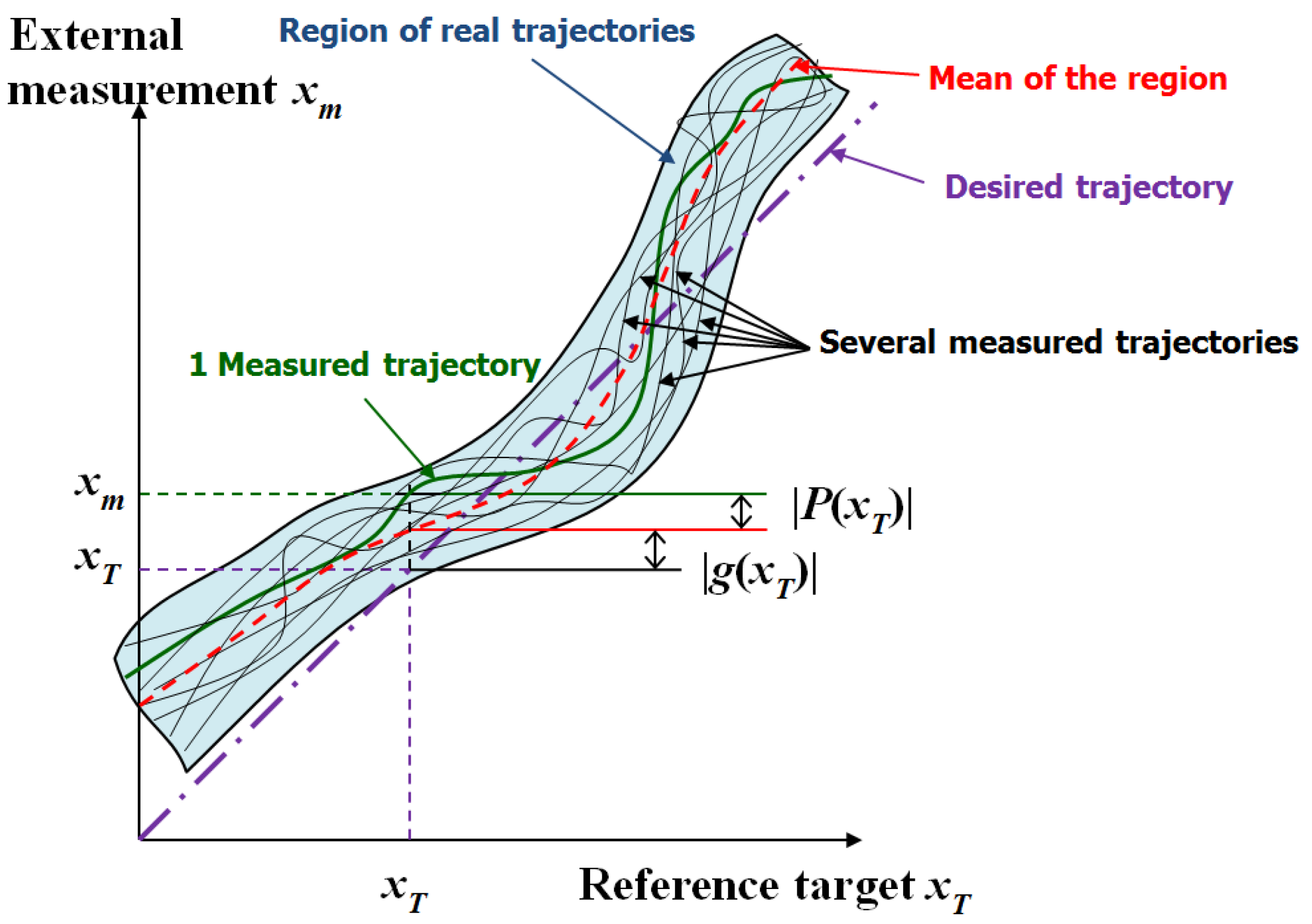
Without loss of generality, the following calculation and analysis will be based on 1-DoF (Degree-of-Freedom) nanopositioning stage which is easy to expand to multi-DoF. Given the target input $x_T$, the real position $x_m$ of the 1-DoF nanopositioning stage is measured by an external sensor and defined by:

$$\begin{array}{c}\hfill x_m=P\left(x_T\right)+x_T+g\left(x_T\right)+D\left(t\right)\end{array}$$

(1)

where $D\left(t\right)$ is the drift induced by environment (we will consider thermal effect) acting on the nanopositioning stage; $g\left(x_T\right)$ is the intrinsic error component inherent in the stage, which results from the control precision of actuator layer which is affected by controller capability and resolution of internal sensor and cannot be compensated by calibration; $P\left(x_T\right)$ is the position-dependent error corresponding to the target input $x_T$. 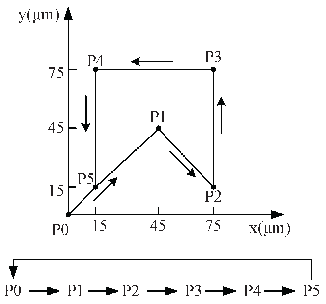Figure 1 shows the geometric representation of every component of input-output of the 1-DoF nanopositioning stage without thermal drift $D\left(t\right)$. $P\left(x_T\right)$ can be minimized by robot calibration. $g\left(x_T\right)$ can be minimized by design, fabrication and control.

Figure 1. Geometric representation of every component of input-output of the 1-DoF nanopositioning stage without thermal drift $D\left(t\right)$.

Figure 1. Geometric representation of every component of input-output of the 1-DoF nanopositioning stage without thermal drift $D\left(t\right)$.

Given a pose, the accuracy expresses the deviation between the command target $x_T$ and the mean of a set of measured poses $\overline{x_m}=\frac{1}{n}{\sum }_{i=1}^n{x}_{mi}$ when reaching the target n times. The 1D accuracy ($Acc$) can be calculated:

$$\begin{array}{ccc}\hfill Acc& =& \left|\overline{x_m}-x_T\right|=\left|\frac{1}{n}\sum _{i=1}^n{x}_{mi}-x_T\right|\hfill \\ \mathrm{(2)}& & =& \left|g\left(x_T\right)+\frac{1}{n}\sum _{i=1}^n{P}_i\left(x_T\right)+\frac{1}{n}\sum _{i=1}^n{D}_i\left(t\right)\right|\hfill \end{array}$$

The positioning repeatability ($Rep$) is expressed as:

$$\begin{array}{ccc}\hfill Rep& =& \frac{1}{n}\sum _{i=1}^n\left|x_{mi}-\overline{x_m}\right|+3\sigma \hfill \\ \mathrm{(3)}& & =& \frac{1}{n}\sum _{i=1}^n\left|P_i\left(x_T\right)-\frac{1}{n}\sum _{j=1}^n{P}_j\left(x_T\right)+D_i\left(t\right)-\frac{1}{n}\sum _{j=1}^n{D}_j\left(t\right)\right|+3\sigma \hfill \end{array}$$

with σ the standard deviation.

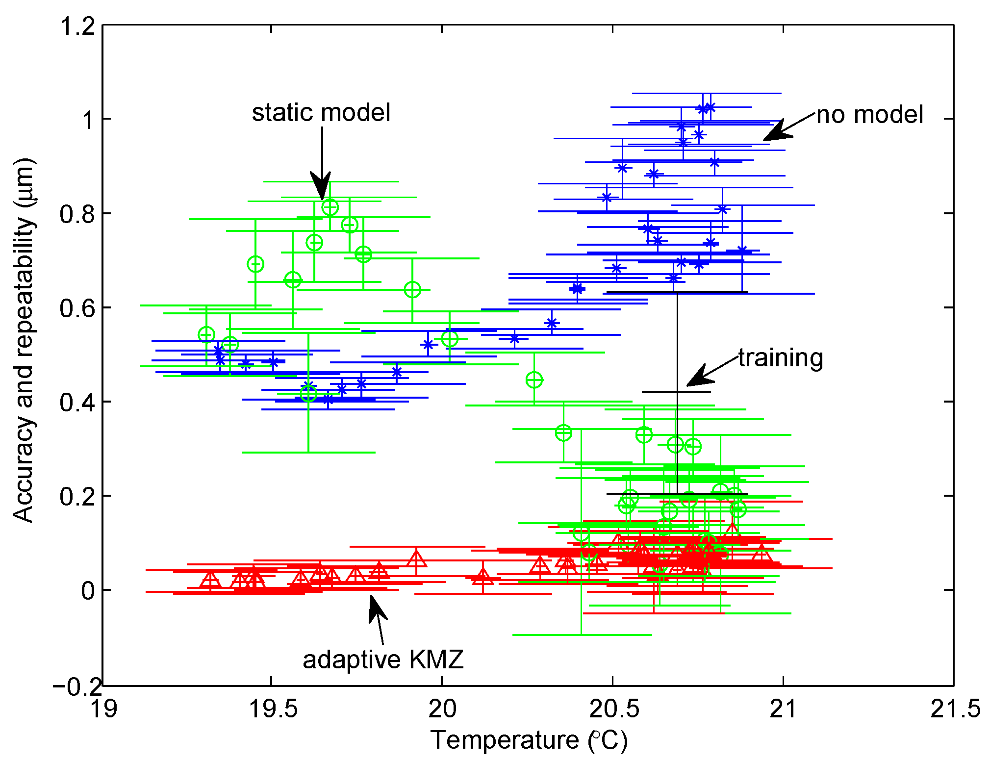
Under external disturbances, the accuracy of the micropositioning stage using calibration is degraded by intrinsic errors and residual errors of imperfect compensation based on the assumption of completely compensating the geometric error; the repeatability is a combination of the intrinsic part and the extrinsic part represented by residual drift.

$$\begin{array}{c}\hfill Ac{c}_S=\left|\frac{1}{n}\sum _{i=1}^n{P}_i\left(x_T\right)+\frac{1}{n}\sum _{i=1}^n{C}_i\left(t\right)\right|\end{array}$$

(4)

$$\begin{array}{ccc}\hfill Re{p}_S& =& \frac{1}{n}\sum _{i=1}^n\left|P_i\left(x_T\right)-\frac{1}{n}\sum _{j=1}^n{P}_i\left(x_T\right)+C_i\left(t\right)-\frac{1}{n}\sum _{j=1}^n{C}_i\left(t\right)\right|+3{\sigma }_S\hfill \end{array}$$

(5)

where subscript “S” represents the static model and $C_i\left(t\right)$ is the residual thermal errors after thermal compensation. Ideally, it is zero, but due to the imperfection of the thermal compensation, $C_i\left(t\right)$ is usually not equal to zero.

And, the final accuracy and repeatability are determined by the maximum values of the test with M testing poses:

$$Acc=max\left(Ac{c}_i\right),i=1,2,\dots ,M$$

(6)

$$Rep=max\left(Re{p}_i\right),i=1,2,\dots ,M$$

(7)

3. Calibration of 1-DoF Nanopositioning Stage

3.1. Geometric Modeling

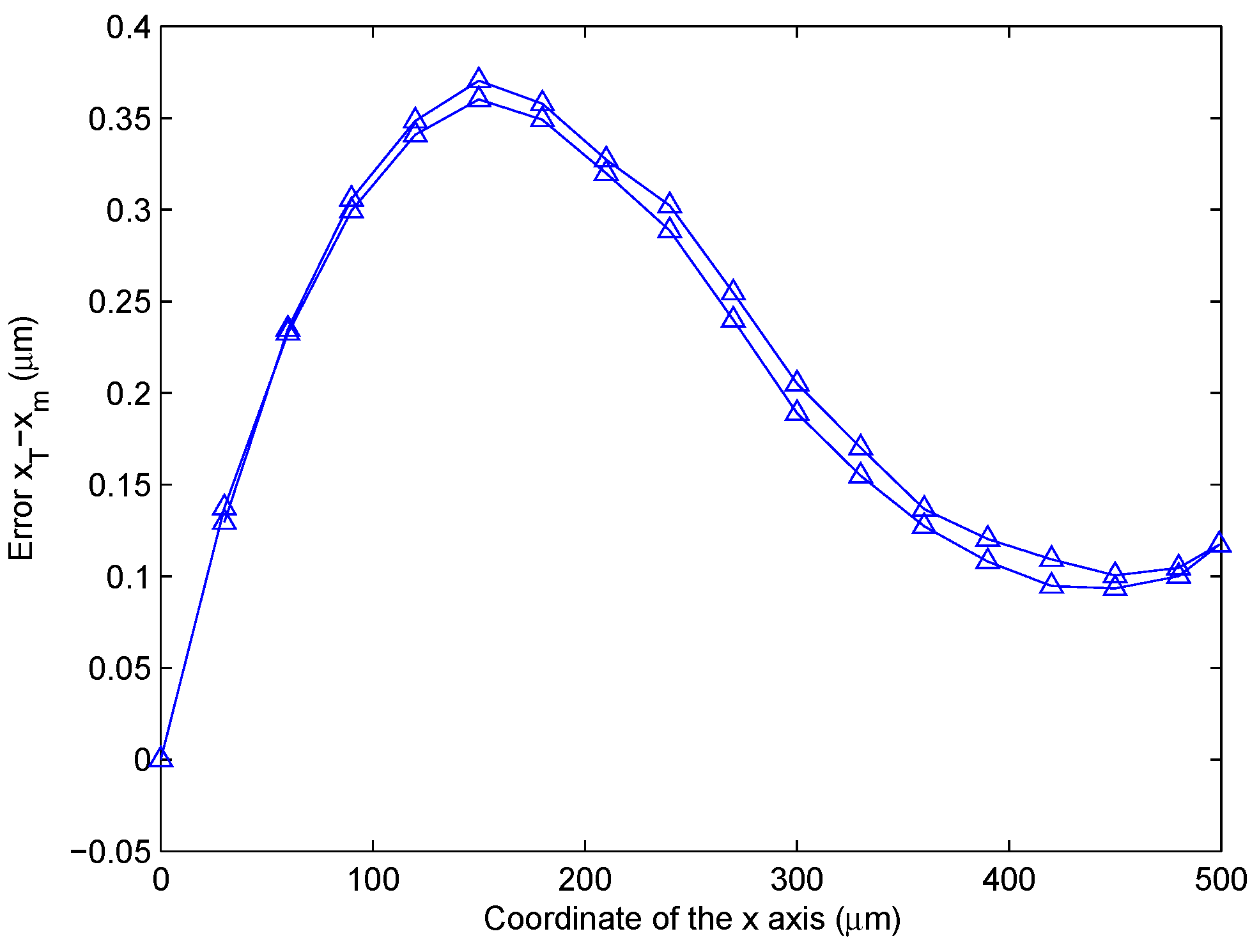
The modeling of nonlinearity errors inherent in the nanopositioning stage is called geometric modeling. To model such errors, a preliminary measurement of the error behavior should be conducted. To do that, the nanopositioning stage is controlled to reach some positions and actual positions are measured by an external sensor (in this case, an interferometer). Figure 2 shows the measured position-dependent errors of a nanopositioning stage. In this case, the curve of errors is a cubic function (3rd order) with two critical points. It is worth mentioning that positioning errors are significant (up to 400 nm) for nanopositioning purposes, even though the stage is already closed loop controlled at the actuator layer. This error is repeatable and then can be compensated through calibration to reach down to a few tens of nanometers.

Figure 2. Geometric errors of the nanopositioning stage where $x_T$ is the target, $x_m$ is the measured position along x. The lower curve corresponds to forward motion while the bottom one to the backward.

Figure 2. Geometric errors of the nanopositioning stage where $x_T$ is the target, $x_m$ is the measured position along x. The lower curve corresponds to forward motion while the bottom one to the backward.

Because of the simple structure of the 1-DoF stage, we can investigate inverse kinematic modeling directly instead of first forward kinematics and then inverse kinematics. The following model is chosen:

$$q_g=\sum _{i=1}^{n1}{a}_i{x}^{n1-i+1}$$

(8)

where $q_g$ is the joint input of the robot; x is the measured position by the external sensor; $a_1,\dots ,a_{n1}$ are geometric coefficients; $n1$ is the order of the geometric model (here, $n1$ = 3).

3.2. Thermal-Drift Modeling

There are two main sets of methods for thermal-drift modeling, namely principle-based and empirical-based methods. The heat transfer model of the compact and small-sized system is very complex, which is difficult if is not impossible to establish analytically and specifically for robots. Hence, we used the latter one because of the fact that empirical-based methods are more appropriate for modeling the relation between the temperature variance and part deformation. This paper emphasizes and focuses on quasi-static calibration problems that directly impact the positioning accuracy of the stages. Such a consideration is valid under certain assumptions that are usually normal when operating nanopositioning stages, for example, when manipulation tasks (e.g., assembly and bonding operations) are carried out at equilibrium or at low-speed (quasi-equilibrium) states [35].

Because the dynamic control is a key issue for applications requiring nanopositioning (for example, scanning probe microscopy), models presented in this paper may also be combined with dynamic control. In this case, the proposed control mode based on calibration approach would act on the positioning accuracy while the internal control loop would act on the transient part. These two control modes would be fully complementary. The closed-loop control of the nanopositioning stage is based on sensory feedback which provides indirect measurements inducing inaccuracies as what Figure 2 shows. Basically, the thermal drift varies slowly and is mainly related to the mechanical structure.

3.2.1. Thermal-Drift Measurement

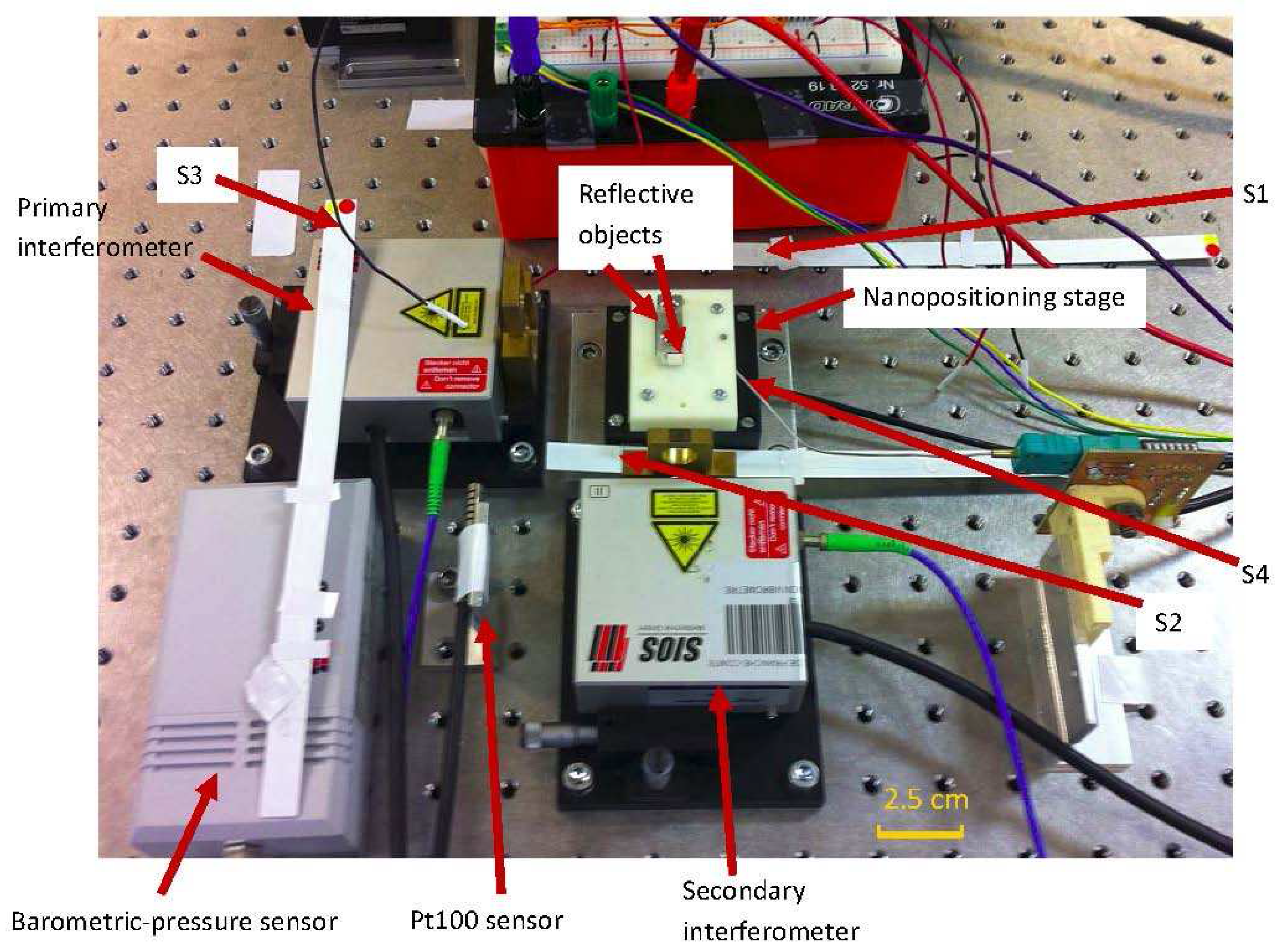
Except for geometric errors, the system is also highly susceptible to thermal disturbances. To choose a suitable calibration model considering thermal effect, we first perform an experiment to characterize the relation between the temperature and drift. In this experiment, the interferometer is used to measure the position of the switched-off nanopositioning stage useful to focus mainly on thermal elongation. The interferometer is defined as a global frame in two days of measurement. Even though without inputting moving commands, the interferometer detects the drift of the stage. 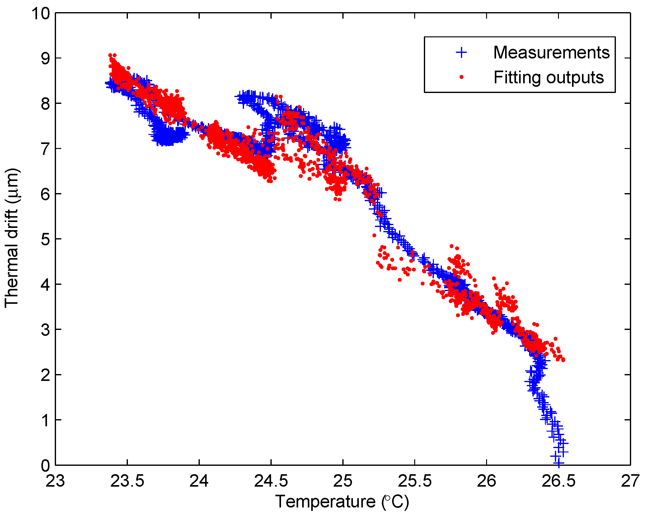Figure 3 shows that the drift increases when the ambient temperature (corresponding to S4 in Figure 6) decreases oppositely. The temperature measurement of one sensor only reflect the temperature change nearby. However, the thermal drift is affected by the temperature change around the stage, which might be due to the thermal effects aggregated from different parts of the setup and surrounding environment. The fitting outputs of the model Equation (10) is the combination of measurements from several sensors. The measurements of all the thermocouples are similar, but there are still some minor differences. At the microscale, these minor differences are important for precisely building an accurate model. Therefore, the relationship shown in Figure 3 is not completely linear.

Figure 3. Relationship between the thermal drift and temperature during the 2-days measurement in ambient environment.

Figure 3. Relationship between the thermal drift and temperature during the 2-days measurement in ambient environment.

3.2.2. Thermal-Drift Modeling

The drift mainly comes from the thermal elongation δ in different parts of the stage. Considering a ideal and simple case, δ can be computed based on the following equation:

$$\begin{array}{c}\hfill \delta =l-l_0=l·\alpha ·(t-t_0)\end{array}$$

(9)

where $l_0$ is the length at reference temperature $t_0$; α is the thermal-expansion coefficient; l is the length of the component after the temperature change $t-t_0$. The thermal expansions from different parts form the gross thermal drift.

Considering the non-uniform temperature field and combination of thermal expansions, we monitor temperatures at several points of the workspace and have the 1st order thermal-drift model:

$$q_t=\sum _{i=1}^{n2}{b}_i{t}_i+\lambda$$

(10)

where $q_t$ is thermal compensation input; $t_i$ is the ith measured temperature and $b_i$ is the corresponding coefficient; λ plays a role of bias; $n2$ is the total number of temperature sensors. The model correlates the temperature field to the induced drift through coefficients $b_1,\dots ,b_{n2}$. Using this model we can approximate the thermal drift using the temperature information, and the fitting result is shown in Figure 3.

3.3. Static Calibration Model

Combining the geometric and thermal drift models yields the complete model [20]:

$$q=\sum _{i=1}^{n1}{a}_i{x}^{n1-i+1}+\sum _{i=1}^{n2}{b}_i{t}_i+\lambda$$

(11)

Obtaining a high fitting precision (e.g., submicron) requires a set of poses/measuring data for training (which is a process of obtaining the parameters of the model using a set of input-output data):

$$\begin{array}{cc}\hfill \left[\begin{array}{c}{q}_1\\ ⋮\\ q_m\end{array}\right]& =\sum _{i=1}^{n1}{a}_i\left[\begin{array}{c}{x}_1^{n1-i+1}\\ ⋮\\ x_m^{n1-i+1}\end{array}\right]+\sum _{i=1}^{n2}{b}_i\left[\begin{array}{c}{t}_{i,1}\\ ⋮\\ t_{i,m}\end{array}\right]+\lambda \hfill \end{array}$$

(12)

where m is the number of measurements.

The equation could be written in matrix form

$$\begin{array}{cc}\hfill \left[\begin{array}{c}{q}_1\\ ⋮\\ q_m\end{array}\right]& =\left[\begin{array}{ccccccc}{x}_1^{n1}& x_1^{n1-1}& \dots & x_1& t_{1,1}& \dots & t_{n2,1}\\ ⋮& ⋮& ⋮& ⋮& ⋮& ⋮& ⋮\\ x_m^{n1}& x_m^{n1-1}& \dots & x_m& t_{1,m}& \dots & t_{n2,m}\end{array}\right]\left[\begin{array}{c}{a}_1\\ ⋮\\ a_{n1}\\ b_1\\ ⋮\\ b_{n2}\end{array}\right]+\lambda \hfill \end{array}$$

(13)

To perform training and parameter identification, the stepwise regression (${Matlab}^{\circledR }$, $StatisticsToolbox$™, MathWorks, Natick, MA, USA) is used because it is able to automatically search the coefficient space and keep the most influential ones by calculating the p-value of F-statistic. The algorithm could be implemented conveniently by a Matlab function $stepwisefit$.

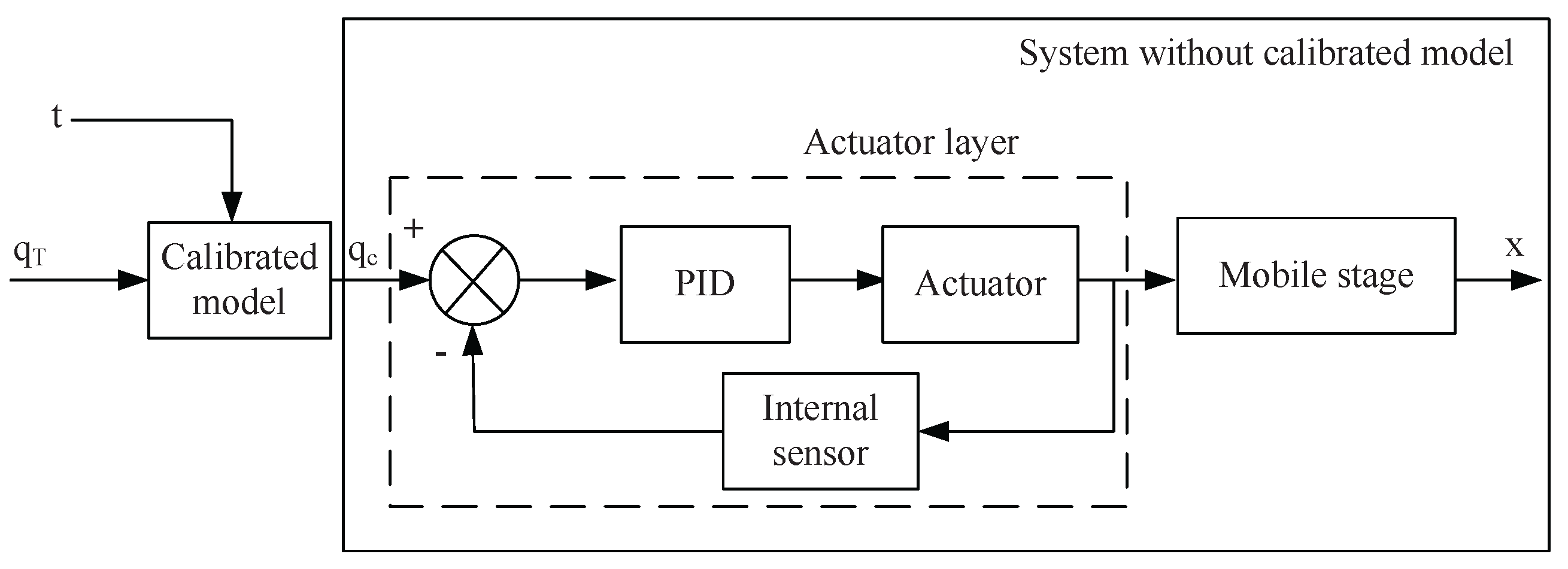
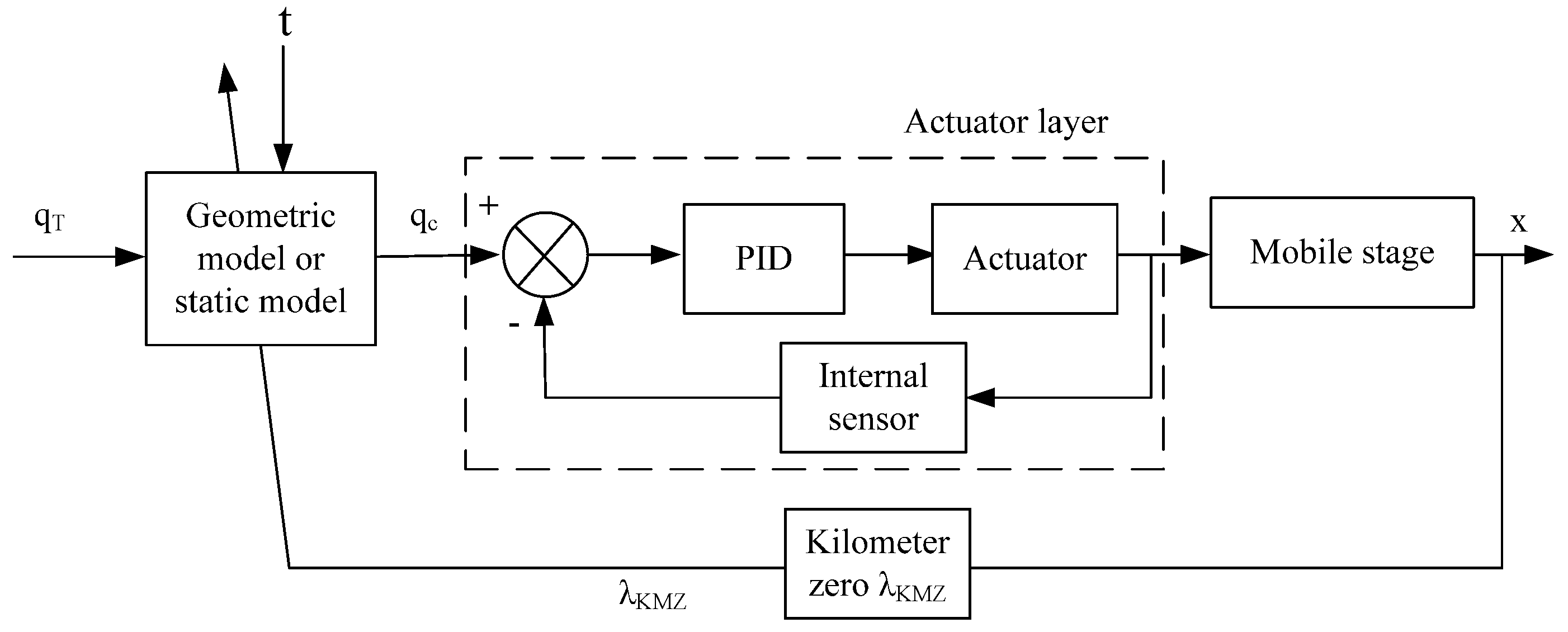
Figure 4 is the block diagram of the nanopositioning stage working in closed loop at actuator layer and in open loop at planning layer. A PID controller is used for the closed loop control. The control input $q_c$ is calculated by the calibrated model with the target $q_T$. In the case without calibrated model, the control input is directly fed with $q_T$.

Figure 4. Block diagram of the nanopositioning stage with the static calibration model.

Figure 4. Block diagram of the nanopositioning stage with the static calibration model.

3.4. Adaptive Model Using KiloMeter-Zero (KMZ)

The thermal behavior is complex and difficult to model accurately, especially at the microscale. On one hand, to perform open loop control, we need to construct the static feedforward model as discussed before. On the other hand, to improve the positioning performance over the long term, we propose an adaptive model to update the compensation of the thermal drift.

Based on the knowledge that the thermal drift is position-independent, we propose to measure the thermal drift at the local position, and then use this information for the compensation along the whole stroke of the stage. To this end, we need to define an absolute frame to which the drift refers. We call this frame KiloMeter-Zero (KMZ). The frame can be defined by a sensor performing direct measurements, or a fixed precise tool (e.g., a fixed AFM tip). In this paper, we use the interferometer to define the KMZ. The working principle of the adaptive model using KMZ is as follows:

• The absolute reference point is defined globally as the KMZ using a sensor or a fixed precise tool.
• The KMZ is reached and the measurement of the sensor is recorded.
• After a period of time, the KMZ is re-reached again and the new measurement is recorded. The drift in this period is the difference of two measurements of the sensor.
• The thermal drift is compensated by adding the calculated difference of the two measurements.

One adaptive model can be formulated as:

$$q=\sum _{i=1}^{n1}{a}_i{x}^{n1-i+1}+{\lambda }_{KMZ}$$

(14)

where ${\lambda }_{KMZ}$ is the drift detected by reaching the KMZ. Such a model is a way to update the drift that can evolve with changing temperature during the modeling process. The first term of Equation (14) is the same as that of the static model which compensates for the geometric errors. In the following experimental studies, the adaptive models all refer to Equation (14). In addition, we can also use the following model:

$$q=\sum _{i=1}^{n1}{a}_i{x}^{n1-i+1}+\sum _{i=1}^{n2}{b}_i{t}_i+{\lambda }_{KMZ}$$

(15)

The block diagram of the adaptive model using the KMZ is shown in Figure 5. Since the feedback happens at predefined intervals, the adaptive model is a trade-off solution between open loop and closed loop control in planning layer.

With compensation using the adaptive model, $q_c=x_T+g^{\prime }\left(q_T\right)+D^{\prime }\left(t\right)+{\lambda }_{KMZ}$ replaces $q_T$ as control input. In a given test, the ith measurement corresponding to target $q_T$ is:

$$\begin{array}{c}\hfill x_{mi}=G_i\left(q_c\right)+D_i\left(t\right)=P_i\left(q_T\right)+q_T+{\lambda }_{KMZ}+D_i\left(t\right)\end{array}$$

(16)

The accuracy is

$$\begin{array}{c}\hfill Ac{c}_A=\left|\frac{1}{n}\sum _{i=1}^n{P}_i\left(q_T\right)+\frac{1}{n}\sum _{i=1}^n[{\lambda }_{KMZ}+D_i\left(t\right)]\right|\end{array}$$

(17)

where subscript “A” stands for the adaptive model and ${\lambda }_{KMZ}$ is only measured at the first zero position, so ${\lambda }_{KMZ}$ = $-D_1\left(t\right)$, when $q_T$ = 0. Then the accuracy becomes

$$\begin{array}{c}\hfill Ac{c}_A=\left|\frac{1}{n}\sum _{i=1}^n{P}_i\left(q_T\right)+\frac{1}{n}\sum _{i=2}^n[{\lambda }_{KMZ}+D_i\left(t\right)]\right|\end{array}$$

(18)

If $D_i\left(t\right)$, $i\ne 1$ is very close to $D_1\left(t\right)$, then ${\lambda }_{KMZ}$=$-D_i\left(t\right)$.

$$\begin{array}{c}\hfill Ac{c}_A=\left|\frac{1}{n}\sum _{i=1}^n{P}_i\left(q_T\right)+{\delta }_A\right|,{\delta }_A⟶0\end{array}$$

(19)

Therefore, if the temperature change is very small, the accuracy after compensation could be at the level without geometric error and external drift which is the highest accuracy theoretically. However, in most cases, the temperature change is not small in the long term. Moreover, because temperature change is relatively slow in the normal micromanipulation laboratories, the frequency of visiting the KMZ could be adjusted based on the temperature magnitude and changing rate.

Figure 5. Block diagram of the system with adaptive model using KMZ.

Figure 5. Block diagram of the system with adaptive model using KMZ.

3.5. Robustness Criterion

There are some works tackling calibration of macro or micro robots with thermal compensation. However, few of them investigate the robustness of calibration which is very important for practical applications. To evaluate robustness of calibration, we propose the following definition:

Definition 1. 

Robustness is defined as the outstanding degree and uniformity of the calibration, which is classified into two types, namely space and time robustness.

Space robustness defines the uniformity of the positioning accuracy of different positions in the whole workspace. The calculation equation is:

$$R_s=\frac{1}{n}\sum _{i=1}^n[max\left(Ac{c}_i\right)-min\left(Ac{c}_i\right)]$$

(20)

which evaluates the sum of deviations between the maximum and minimum accuracies of all tests in a period of time.

Time robustness defines the uniformity of the positioning accuracy in the whole process. The calculation equation is:

$$R_t=\frac{\frac{1}{n}{\sum }_{i=1}^{n}max\left(Ac{c}_i\right)}{\text{Time}}$$

(21)

which evaluates the sum of maximum accuracies of all tests in a period of time.

If the values of $R_s$ and $R_t$ are smaller, the space and time robustness is better.

4. Experimental Study

4.1. Experimental Setup

As shown in Figure 6, the experimental setup consists of a single-axis nanopositioning stage P-625.1CD (Physik Instrumente, Karlsruhe, Germany), two laser interferometer sensor heads (SP-S 120, SIOS Meßtechnik GmbH, Ilmenau, Germany) with a resolution of 0.3 nm, four K-type thermocouples and a barometric pressure sensor. The nanopositioning stage is controlled in closed-loop (PID) at actuator layer with internal capacitive sensor. The positioning resolution given by the manufacturer is 1.4 nm. The interferometer defines the global frame during training and validation by setting the initial reading at the beginning of training phase as zero.

Figure 6. Experimental setup comprising one single-axis nanopositioning stage and reflective object, two interferometers with affiliated pressure/temperature sensors, four temperature sensors.

Figure 6. Experimental setup comprising one single-axis nanopositioning stage and reflective object, two interferometers with affiliated pressure/temperature sensors, four temperature sensors.

The three main measuring uncertainties of the interferometer system come from the wavelength compensation, deadpath correction and material thermal compensation. Here, wavelength compensation and deadpath correction are realized by built-in temperature/pressure-correction module (incorporates a temperature sensor Pt100 and barometric-pressure sensor as seen in Figure 6). Sensor noise is one of the major sources in nanopositioning systems [36]. According to the calculation method in GUM (Guide to the Expression of Uncertainty in Measurement) [37], we calculate the measurement uncertainty of the interferometer less than 41 nm considering intrinsic and extrinsic factors.

Four thermocouples (S1 → S4) are placed around the nanopositioning stage to monitor the temperature change. Even though the measurements of these thermocouples are close, there are still some minor differences. At the microscale, these minor differences are important for precise building of an accurate model. Hence, several thermocouples are required. So far, nobody has succeeded in defining where the good locations are to be measured. In addition, the experimental setup is covered by a shield against air flow.

Figure 7 shows the hardware allocation and signal flow. The controller sends the command q to the nanopositioning stage and receives measurement $x_{internal}$ from internal sensor for closed loop control in actuator layer. The stage reaches position $x_{real}$, $y_{real}$. Measurements $x_m$, $y_m$ are obtained by interferometers. Dspace board connected with the PC is the hub of signal flow.

Figure 7. Schematic diagram of the hardware allocation and signal flow.

Figure 7. Schematic diagram of the hardware allocation and signal flow.

4.2. Procedures of Calibration and Validation

The whole procedure of the calibration using the static model is shown in Figure 8, which includes measurement, training, and validation phases. In the measurement phase, a few target points q along the axis are defined; the nanopositioning stage is controlled to reach these positions; the external sensor records the real position x and the thermocouples record the temperature t during this phase. Subsequently, based on the inverse model, parameters are identified using all information (q, x, and t). For implementing the calibrated model, we first define target points $x^{\prime }$, and then calculate the corresponding joint coordinates $q^{\prime }$ using the identified parameters and the model. The nanopositioning stage is controlled to move for performance validation. Finally, the real positions $x^{″}$ are measured and used to calculate the accuracy achieved.

Firstly, we need to acquire position information for model training through external measurement. The workspace of the nanopositioning stage is a line of 500 μm. We define the joint coordinates of the moving trajectory (named training trajectory) from 0 to 480 μm with a stepsize of 30 μm. The control trajectory is shown in Figure 9 which demonstrates that, in every cycle, the rising time of the input signal is 2 s and the input keeps constant 20 s before the next in order to have stable state. The average values in the last 5 s of every step are considered as the measurements x and used for training. Meanwhile, four thermocouples obtain a set of temperature data t. Data acquisition takes about 12 h for 24 cycles. All the data are fed into Stepwise algorithm for training. Afterwards, the identified parameters Φ (including $a_i$, $b_i$ and λ) are embedded into the controller. The test points $x^{\prime }$ for validation are taken at coordinates (0, 80, 160, 240, 320, 400, 480) μm. These points include the ones (0, 240, 480) also considered in the training phase and the ones (80, 160, 320, 400) never used for training. Validating the points both inside and outside the training set helps to evaluate performances of both robustness and generalization (or interpolation). Every test of validation takes 1.25 h for 15 cycles.

Figure 8. Flow chart of calibration of nanopositioning stages.

Figure 8. Flow chart of calibration of nanopositioning stages.

Figure 9. Command trajectories for training and validation in 1 cycle.

Figure 9. Command trajectories for training and validation in 1 cycle.

4.3. Experimental Results and Discussions

4.3.1. Performance under Stable Temperature

The first experiment is testing the positioning accuracy and repeatability of the nanopositioning stage in a controlled environment with temperature control in order to decouple the geometric errors and the thermal effect. The temperature is controlled within ±0.05 ${}^{\circ }C$ inside the room. The positioning accuracy 350 nm showed in Figure 10 is the intrinsic accuracy. This value results from the intrinsic and position-dependent errors. In the constant temperature, this value keeps relatively constant. The difference between the accuracies of the forward and backward motion is quite small (about 10 nm) which means the hysteresis of the stage has been eliminated well by the closed loop control in actuator layer. The corresponding repeatability is about 35 nm. This value is induced by the controller and internal sensor which is considered as the intrinsic characteristics of the stage.

Figure 10. Accuracy of the nanopositioning stage in a controlled environment.

Figure 10. Accuracy of the nanopositioning stage in a controlled environment.

4.3.2. Performances under Varying Temperature

The calibration procedure follows the flow chart in Figure 8. The duration of the training step is about 14 h with 67 cycles of forward and backward motions. Every cycle = 18 poses (forward) + 16 poses (backward). After achieving the training, identified parameters of the model are obtained and shown in Table 1. Validation tests are then performed which aim at quantifying performances of the calibrated nanopositioning robot. Every validation test takes 1.25 h for 15 cycles of forward and backward motions. Validation tests are performed in the repeating order of: with no calibration (the model equation is $q=x$), with adaptive model using KMZ, and with static model. Here the KMZ is measured every 3.75 h.

Table 1. Identified parameters of static model.

Parameters	Values
$a_1$	2.454 ×${10}^{-8}$
$a_2$	−2.167 ×${10}^{-5}$
$a_3$	1.005
$b_1$	2.978
$b_2$	−3.142
$b_3$	−0.996
$b_4$	0.690
λ	10.413 (μm)

Table 1. Identified parameters of static model.

Parameters	Values
$a_1$	2.454 ×${10}^{-8}$
$a_2$	−2.167 ×${10}^{-5}$
$a_3$	1.005
$b_1$	2.978
$b_2$	−3.142
$b_3$	−0.996
$b_4$	0.690
λ	10.413 (μm)

Among the accuracies of 34 poses in the training phase (TP), the maximum value is more than 450 nm and the minimum is about 150 nm in forward and backward motions as depicted in Figure 11. Accuracies of different poses in the first validation test (T1) are quite different in the curves with no calibration. The difference between the maximum (650 nm) and minimum (350 nm) is about 300 nm, which is close to that of TP. Both of the accuracy curves of TP and T1 have a similar shape as well as that in Figure 10. This is because thermal effect acts on all the positions and deviates them equivalently. The second (T2) and third (T3) tests are using the adaptive model using KMZ, and the static model, respectively. The largest accuracies are about 43 nm in T2 and 95 nm in T3, which are much smaller than those without calibration. The difference is about 35 nm in T2 and is about 40 nm in T3. These results show that the two models not only improve the overall accuracy, but also decrease the accuracy differences of test points in the workspace.

Figure 12 shows the accuracy evolution of all validation points during the experiment having a five days duration. The accuracy of no calibration reaches 1 μm and stays larger than 400 nm during the whole process. These results suffer from the temperature influence, which is different from that (<400 nm) in Figure 10 where temperature influence is negligible. The static model performs good positioning accuracy (smaller than 400 nm) in the first 70 h and deteriorates afterwards. The adaptive model using KMZ achieves accuracy always better than 100 nm. Hence, the adaptive and static models can provide much better performance than no calibration. If long-term good performance is required, the adaptive model should be used.

Figure 11. Accuracy of the training phase (TP) and first three tests (T1, T2, and T3).

Figure 11. Accuracy of the training phase (TP) and first three tests (T1, T2, and T3).

Figure 12. Accuracy evolution of all validation poses in five days. Time 0 = end of training = start of validation.

Figure 12. Accuracy evolution of all validation poses in five days. Time 0 = end of training = start of validation.

Figure 13 shows the temperature evolution inside the experimental room during the validation. Temperature change is relatively regular in first 60 h, and the variations are about 0.2∼0.3 ${}^{\circ }C$ which is basically within the temperature range of training phase. In the latter two days, temperature changes 1.3 ${}^{\circ }C$. Figure 14 illustrates the relationship between temperature and accuracy/repeatability.

Combining Figure 12, Figure 13 and Figure 14, it is observed that the accuracies of the adaptive model are not sensitive to temperature change no matter whether the temperature is in the range of training or not. In the first 70 h, the accuracies of the static model are almost better than 300 nm when the temperature is within the range of the training phase. However, the accuracy is getting much worse, which is due to the fact that the temperature afterwards changed out of the range of the training phase. This means the performance of the static model largely depends on the training information. Hence, if the drift behavior and temperature range after training are close to those during training, the static model can provide efficient compensation based on previous knowledge. Based on this, for practical application, we should consider carefully the information gotten and design better procedure during the training phase when going to use the static model. In contrast, the adaptive model is able to update the new information that thermal drift can be compensated efficiently in spite of how temperature changes.

Figure 13. Evolution of the room temperature in five days.

Figure 13. Evolution of the room temperature in five days.

Figure 14. Relationship between temperature and accuracy and repeatability.

Figure 14. Relationship between temperature and accuracy and repeatability.

Based on the definitions in Section 3.5, the space and time robustness are calculated and shown in Table 2. The quantified robustness shows clearly that adaptive model using KMZ works better than other two, with smallest robustness indices in terms of space and time. The static model works very well for geometric errors compensation with small value of space robustness but not well when the temperature varies with bad time robustness. Therefore, it would be interesting that the geometric calibration conducted by the device manufacturers combines with KMZ method conducted by the users using internal low cost sensors for applications requiring a very good accuracy.

Table 2. Robustness of calibration of the nanopositioning stage.

Robustness	No Model	Static Model	Adaptive Model
Space robustness $R_s$	0.3476	0.0577	0.0493
Time robustness $R_t$	0.0058	0.0029	0.0005

Table 2. Robustness of calibration of the nanopositioning stage.

Robustness	No Model	Static Model	Adaptive Model
Space robustness $R_s$	0.3476	0.0577	0.0493
Time robustness $R_t$	0.0058	0.0029	0.0005

5. Calibration of Multi-DoF Nanopositioning Stage

The above study of 1-DoF calibration of nanopositioning stage can be extended to multi-DoF study of coupling effects. This section illustrates the extension of static model to multi-DoF case (with a P-611.3 NanoCube Piezo Stage).

5.1. Modeling of 2-DoF Nanopositioning Stage

Similar to the 1-DoF nanopositioning, the 2-DoF stage is also modeled with polynomials. The difference from 1-DoF is the consideration and compensation of coupling errors from one axis to another. We define the following model for the 2-DoF nanopositioning stage:

$$\begin{array}{c}\hfill \left\{\begin{array}{c}{q}_x=\sum _{i=1}^{n1}{a}_{ix}{x}^i+\sum _{i=1}^{n2}{b}_{ix}{y}^i+\sum _{i=1}^{n3}{c}_{ix}{t}_i+{\lambda }_x\hfill \\ q_y=\sum _{i=1}^{n1}{a}_{iy}{x}^i+\sum _{i=1}^{n2}{b}_{iy}{y}^i+\sum _{i=1}^{n3}{c}_{iy}{t}_i+{\lambda }_y\hfill \end{array}\right.\end{array}$$

(22)

where $a_{ij}$ is the ith coefficient for modeling errors along j axis induced by X motion; $b_{ij}$ is the ith coefficient for modeling errors along j axis induced by Y motion; $c_{ij}$ is the ith coefficient for modeling thermal drift along j axis; ${\lambda }_j$ is the offset term along j axis.

5.2. Experimental Study of 2-DoF Nanopositioning Robot

5.2.1. Procedures of Calibration and Validation

Figure 15 shows the trajectory of joint space for data acquisition for model training. The measurements are taken at positions 0:10:80 μm along XY and 81 pairs of measurements are obtained in every cycle. At the end of every cycle, the nanopositioning robot is controlled to go back to the start point from the end point. In total, 12 cycles are finished during 6 h of training phase.

Five points ($P_1$, …, $P_5$) never used for training plus the origin $P_0$ are chosen for validation (Figure 16). The coordinates of these points are $(0,0)$, $(45,45)$, $(75,15)$, $(75,75)$, $(15,75)$, and $(15,15)$ μm. The nanopositioning stage is controlled from $P_0$ to $P_1$, …, $P_5$ in turn, and then goes back to $P_0$ for a new cycle.

Figure 15. Trajectory of data acquisition for model training.

Figure 15. Trajectory of data acquisition for model training.

Figure 16. Coordinates and trajectory of six points for validation.

Figure 16. Coordinates and trajectory of six points for validation.

5.2.2. Experimental Results

Figure 17 shows the overall accuracy and repeatability of 2-DoF nanopositioning stage. The accuracy value in the training phase is larger than 1.4 μm. After training, performance tests are performed with and without using the calibration model Equation (22). In nearly one day, the accuracy of no calibration is always about 1.2∼1.4 μm which is in quite the same range as the accuracy in training phase. Using the calibrated model, most of the accuracies keep better than 200 nm and all of them are better than 500 nm. The temperature evolution during this time is shown in Figure 18. When temperature changes within the range as the training temperature, accuracy can even be better than 200 nm which is much superior to that (1400 nm) without using model.

Figure 17. Experimental accuracy and repeatability of 2-DoF nanopositioning stage in training and validation phases. Time 0 = end of training = start of validation.

Figure 17. Experimental accuracy and repeatability of 2-DoF nanopositioning stage in training and validation phases. Time 0 = end of training = start of validation.

Figure 18. Temperature evolution in training and validation phases.

Figure 18. Temperature evolution in training and validation phases.

6. Conclusions

Nanopositioning systems usually suffer from geometric errors due to imperfect actuator behavior. In addition, thermal drift is also a major source of inaccuracy. To improve the nanopositioning accuracy, we need to compensate for the geometric errors and thermal drift. This paper presented theoretical formulations, modeling discussions, and experimental validation results. A static model and an adaptive model have been proposed. The static model depicted the geometric errors and thermal drift in a static structure. The adaptive model was able to compensate for thermal drift by updating the drift information through revisiting the kilometer-zero. Based on measurements of interferometer and thermocouples, a set of experiments have been conducted to characterize, to calibrate, and to validate the performances of the nanopositioning stage.

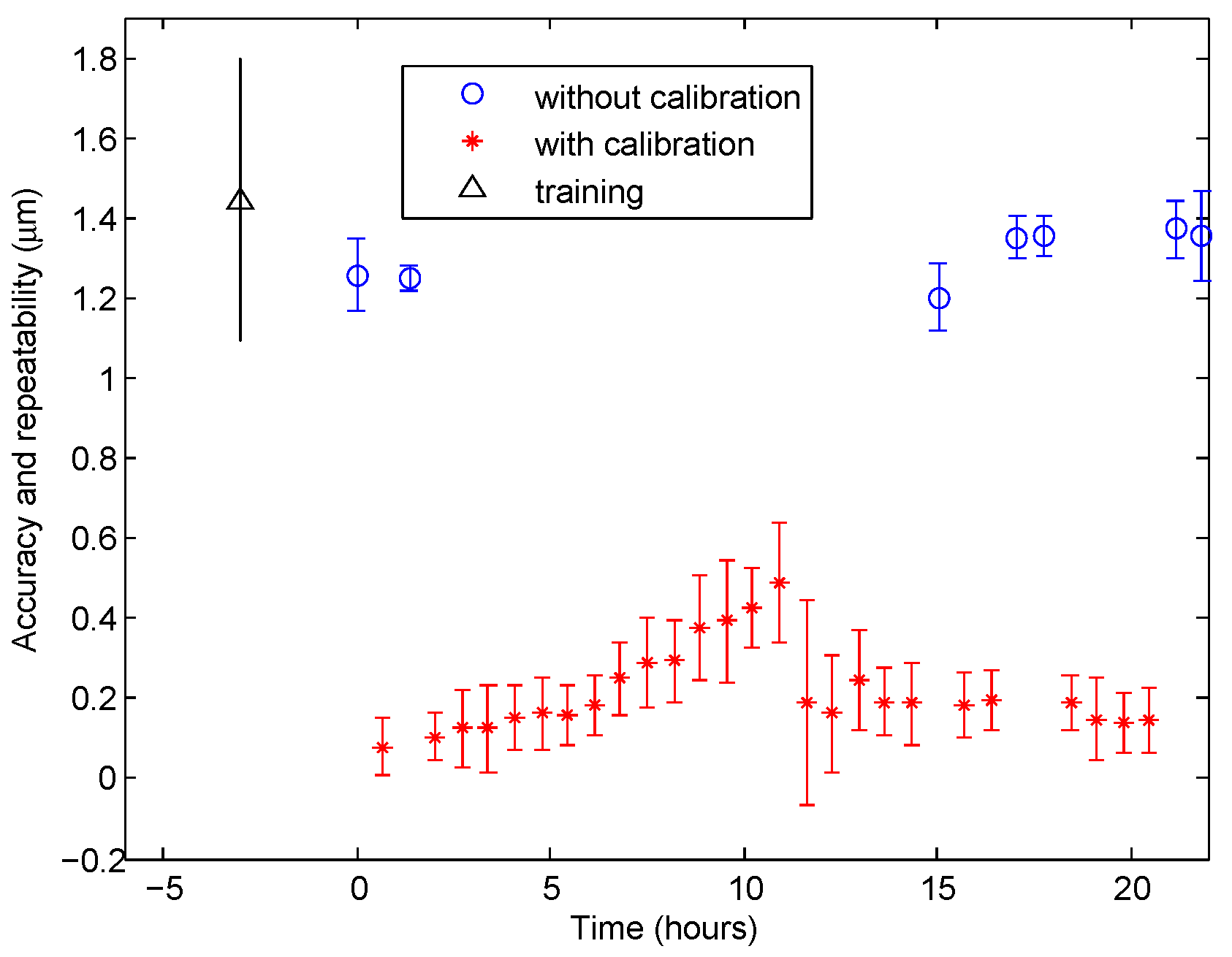
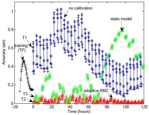
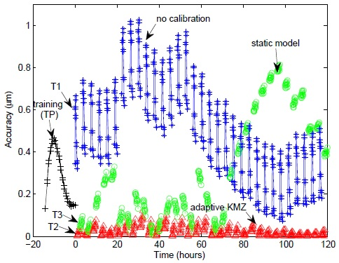
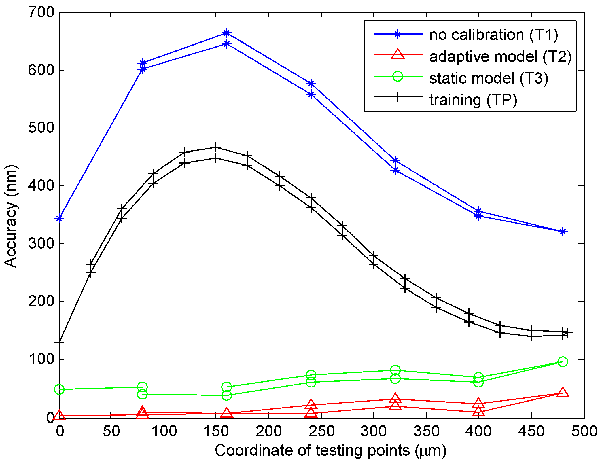
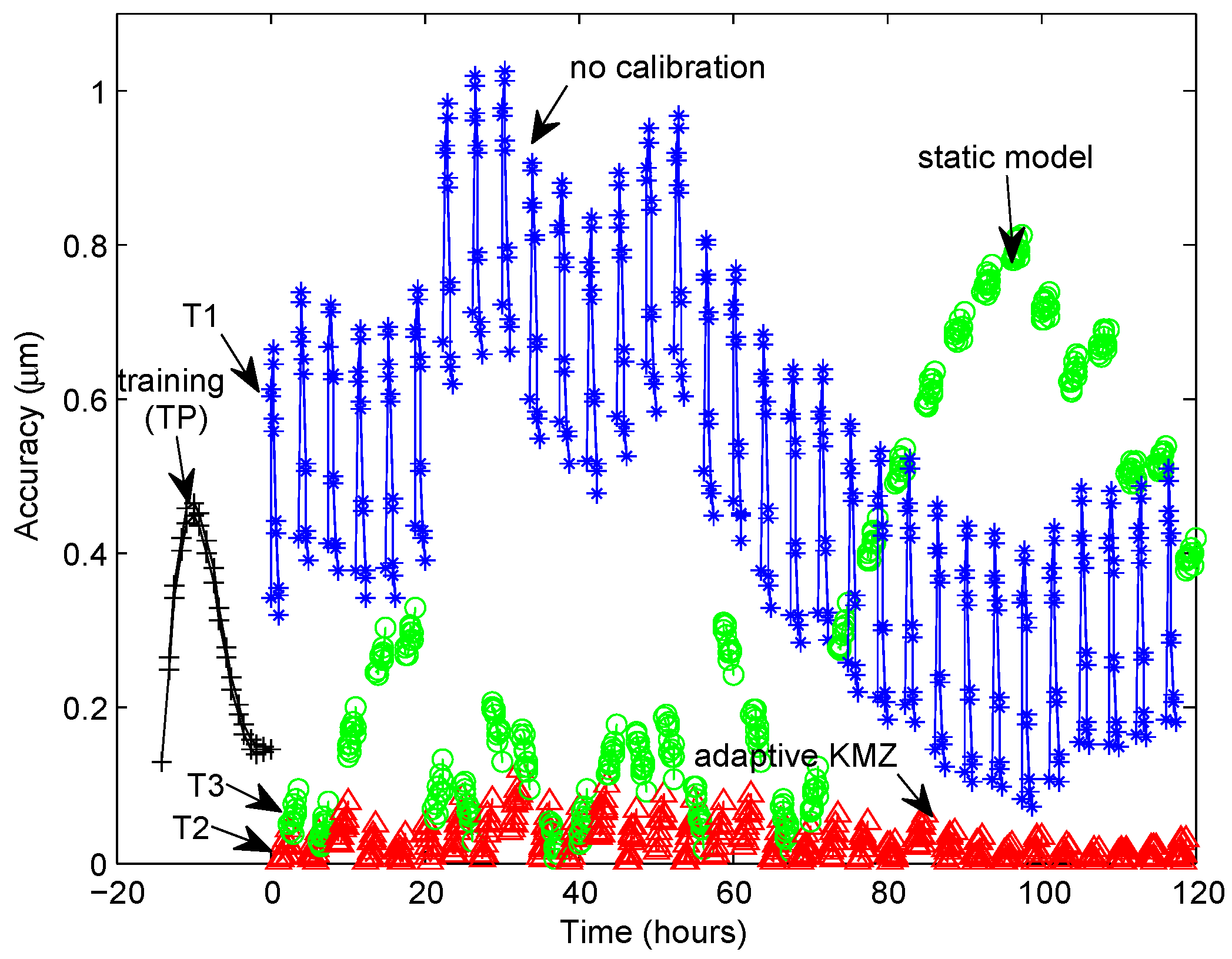
The experimental results demonstrated that the performance of the static model depended largely on the consistency of conditions before and after training. If the drift behavior and temperature range after training were close to those during training, the static model can guarantee efficient compensation based on training knowledge. Results showed that accuracy was better 400 nm in this case. The adaptive model was able to update the new information that thermal drift can be compensated efficiently in spite of how temperature changes. The achieved accuracies were almost better than 100 nm. On the other side, without compensation, accuracy could be up to 1 μm even if temperature did not go far away from the training range. Calculation of time and space robustness provided numerical comparisons of two models and no model. In addition, we extended the 1-DoF calibration to multi-DoF with a case study of a 2-DoF nanopositioning robot. Results also demonstrated that the model efficiently improved the 2D accuracy from 1400 nm to 200 nm.

Future work will be using a low cost (high resolution, small range) sensor, which is able to measure accurately in a very small space to integrate in the stages.

References

1. Garza, H.H.P.; Ghatkesar, M.K.; Basak, S.; Löthman, P.; Staufer, U. Nano-Workbench: A Combined Hollow AFM Cantilever and Robotic Manipulator. Micromachines 2015, 6, 600–610. [Google Scholar] [CrossRef]
2. Zhang, X.; Koo, B.; Salapaka, S.; Dong, J.; Ferreira, P. Robust Control of a MEMS Probing Device. IEEE/ASME Trans. Mechatron. 2014, 19, 100–108. [Google Scholar] [CrossRef]
3. Nakahara, K.; Sakuma, S.; Hayakawa, T.; Arai, F. On-Chip Transportation and Measurement of Mechanical Characteristics of Oocytes in an Open Environment. Micromachines 2015, 6, 648–659. [Google Scholar] [CrossRef]
4. Zhang, Y.; Han, M.; Yu, M.; Shee, C.Y.; Ang, W.T. Automatic Hysteresis Modeling of Piezoelectric Micromanipulator in Vision-Guided Micromanipulation Systems. IEEE/ASME Trans. Mechatron. 2012, 17, 547–553. [Google Scholar] [CrossRef]
5. Chaillet, N.; Régnier, S. Microrobotics for Micromanipulation; Wiley-ISTE: Hoboken, NJ, USA, 2010. [Google Scholar]
6. Zhu, H.; Fujimoto, H. Mechanical deformation analysis and high-Precision control for ball-screw-driven stages. IEEE/ASME Trans. Mechatron. 2015, 20, 956–966. [Google Scholar] [CrossRef]
7. Wang, H.Y.; Fan, K.C.; Ye, J.K.; Lin, C.H. A Long-Stroke Nanopositioning Control System of the Coplanar Stage. IEEE/ASME Trans. Mechatron. 2014, 19, 348–356. [Google Scholar] [CrossRef]
8. Devasia, S.; Eleftheriou, E.; Moheimani, S.O.R. A survey of control issues in nanopositioning. IEEE Trans. Control Syst. Technol. 2007, 15, 802–823. [Google Scholar] [CrossRef]
9. Li, Y.; Xu, Q. Design and robust repetitive control of a new parallel kinematic XY piezostage for Micro/Nanomanipulation. IEEE/ASME Trans. Mechatron. 2012, 17, 1120–1132. [Google Scholar] [CrossRef]
10. Lin, F.J.; Lee, S.Y.; Chou, P.H. Computed force control system using functional link radial basis function network with asymmetric membership function for piezo-flexural nanopositioning stage. IET Control Theory Appl. 2013, 7, 2128–2142. [Google Scholar] [CrossRef]
11. Rakotondrabe, M.; Clévy, C.; Lutz, P. Complete open loop control of hysteretic, creeped, and oscillating piezoelectric cantilevers. IEEE Trans. Autom. Sci. Eng. 2009, 7, 440–450. [Google Scholar] [CrossRef] [Green Version]
12. Clark, L.; Shirinzadeh, B.; Tian, Y.; Oetomo, D. Laser-based sensing, measurement, and misalignment control of coupled linear and angular motion for ultrahigh precision movement. IEEE/ASME Trans. Mechatron. 2015, 20, 84–92. [Google Scholar] [CrossRef]
13. Clévy, C.; Rakotondrabe, M.; Chaillet, N. Signal Measurement and Estimation Techniques for Micro and Nanotechnology; Springer-Verlag New York: New York, NY, USA, 2011. [Google Scholar]
14. Maroufi, M.; Bazaei, A.; Moheimani, S.O.R. A high-bandwidth MEMS nanopositioner for on-chip AFM: Design, characterization, and control. IEEE Trans. Control Syst. Technol. 2015, 23, 504–512. [Google Scholar] [CrossRef]
15. Teo, T.J.; Yang, G.; Chen, I.M. A flexure-based electromagnetic nanopositioning actuator with predictable and re-configurable open-loop positioning resolution. Precis. Eng. 2015, 40, 249–260. [Google Scholar] [CrossRef]
16. Kara-Mohamed, M.; Heath, W.P.; Lanzon, A. Enhanced Tracking for Nanopositioning Systems Using Feedforward/Feedback Multivariable Control Design. IEEE Trans. Control Syst. Technol. 2015, 23, 1003–1013. [Google Scholar] [CrossRef]
17. Tan, N.; Clévy, C.; Laurent, G.; Chaillet, N. Calibration and validation of XYΘ micropositioners with vision. In Proceedings of the IEEE/ASME International Conference on Advanced Intelligent Mechatronics, Kachsiung, Taiwan, 11–14 July 2012; pp. 256–261.
18. Chen, X.; Li, W. A monolithic self-sensing precision stage: Design, modeling, calibration, and hysteresis compensation. IEEE/ASME Trans. Mechatron. 2015, 20, 812–823. [Google Scholar] [CrossRef]
19. Aktakka, E.; Woo, J.K.; Egert, D.; Gordenker, R.; Najafi, K. A Microactuation and Sensing Platform with Active Lockdown for in Situ Calibration of Scale Factor Drifts in Dual-Axis Gyroscopes. IEEE/ASME Trans. Mechatron. 2015, 20, 934–943. [Google Scholar] [CrossRef]
20. Tan, N.; Clévy, C.; Chaillet, N. Calibration of single-axis nanopositioning cell subjected to thermal disturbance. In Proceedings of the IEEE International Conference on Robotics and Automation, Karlsruhe, Germany, 6–10 May 2013; pp. 3645–3650.
21. Lubrano, E.; Clavel, R. Thermal Behavior of an Ultra High-Precision Linear Axis Operating in Industrial Environment. In Proceedings of the 9th International Workshop on Research and Education in Mechatronics, Bergamo, Italy, 18–19 September 2008; pp. 151–152.
22. Chen, J.S.; Yuan, J.; Ni, J. Thermal Error Modelling for Real-Time Error Compensation. Int. J. Adv. Manuf. Technol. 1996, 12, 266–275. [Google Scholar] [CrossRef]
23. Fraser, S.; Attia, M.; Osman, M. Modelling, Identification and Control of Thermal Deformation of Machine Tool Structures, Part 2: Generalized Transfer Functions. J. Manuf. Sci. Eng. 1998, 120, 632–639. [Google Scholar] [CrossRef]
24. Krulewich, D. Temperature Integration Model and Measurement Point Selection for Thermally Induced Machine Tool Errors. Mechatronics 1998, 8, 395–412. [Google Scholar] [CrossRef]
25. Gong, C.; Yuan, J.; Ni, J. Nongeometric error identification and compensation for robotic system by inverse calibration. Int. J. Mach. Tools Manuf. 2000, 40, 2119–2137. [Google Scholar] [CrossRef]
26. Zhao, H.; Yang, J.; Shen, J. Simulation of Thermal Behavior of a CNC Machine Tool Spindle. Int. J. Mach. Tools Manuf. 2007, 47, 1003–1010. [Google Scholar]
27. Zhu, J. Robust Thermal Error Modeling and Compensation for CNC Machine Tools. Ph.D. Thesis, The University of Michigan, Ann Arbor, MI, USA, 2008. [Google Scholar]
28. Li, J.; Yang, G.; Zhang, W.; Tu, S.; Chen, X. Thermal effect on piezoelectric stick-slip actuator systems. Rev. Sci. Instrum. 2008, 79, 046108. [Google Scholar] [CrossRef] [PubMed]
29. Kim, K.; Heo, J.; Kim, K. Effects of Temperature on the Microscale Adhesion Behavior of Thermoplastic Polymer Film. Tribol. Lett. 2010, 38, 97–106. [Google Scholar] [CrossRef]
30. Das, A.; Murthy, R.; Popa, D.; Stephanou, H. A Multiscale Assembly and Packaging System for Manufacturing of Complex Micro-Nano Devices. IEEE Trans. Autom. Sci. Eng. 2012, 9, 160–170. [Google Scholar] [CrossRef]
31. Mattos, L.; Caldwell, D. A fast and precise micropipette positioning system based on continuous camera-robot recalibration and visual servoing. In Proceedings of the IEEE International Conference on Automation Science and Engineering, Bangalore, India, 22–25 August 2009; pp. 609–614.
32. Zhang, Y.; Han, M.; Shee, C.; Ang, W. Calibration of piezoelectric actuator-based vision guided cell microinjection system. In Proceedings of the IEEE/ASME International Conference on Advanced Intelligent Mechatronics, Xi’an, China, 2–5 July 2008; pp. 808–812.
33. ISO 9283:1998 Manipulating Industrial Robots—Performance Criteria and Related Test Methods; International Organization for Standardization: Geneva, Switzerland, 1998.
34. Tan, N.; Clévy, C.; Chaillet, N. Performance analysis and characterization of micro-nanopositioning systems. Electron. Lett. 2014, 50, 1853–1855. [Google Scholar] [CrossRef]
35. Popa, D.; Murthy, R.; Das, A. M3-deterministic, multiscale, multirobot platform for microsystems packaging: Design and quasi-static precision evaluation. IEEE Trans. Autom. Sci. Eng. 2009, 6, 345–361. [Google Scholar] [CrossRef]
36. Fleming, A.J. Measuring and predicting resolution in nanopositioning systems. Mechatronics 2014, 24, 605–618. [Google Scholar] [CrossRef]
37. Castro, H.F.F. Uncertainty Analysis of a Laser Calibration System for Evaluating the Positioning Accuracy of a Numerically Controlled Axis of Coordinate Measuring Machines and Machine Tools. Precis. Eng. 2008, 32, 106–113. [Google Scholar] [CrossRef]