Analysis of Dynamic Performance of a Kalman Filter for Combining Multiple MEMS Gyroscopes


Abstract
:
1. Introduction
2. Principle Model of the Virtual Gyroscope


 , and qω is the variance of white noise nω. Using a KF technique, setting the true angular rate ω as the system estimated quantity, based on the gyroscope model of Equation (3) and true angular rate model of Equation (5), thus the filtering state-space model for virtual the gyroscope system can be expressed as:


 is the estimate of the system state, K(t) is the filter gain, and P(t) is the estimated covariance. Previously, an analytic approach was used to solve the continuous-time KF from Equation (7) to Equation (9) in [13], and led to a steady-state covariance and gain, thus the discrete-time KF for rate signal estimate can be given as:

 and the matrix Q = C−1·(1 − α)·HTR−1 (here β is the component values of the matrix Q), then the discrete-time KF of Equation (10) can be expressed as:

 and system measurement ZK+1, which satisfies the relationship of α + N·β = 1.0. Equation (11) shows that the values of factors α and β are mainly determined by the parameter qω. The expression of factor α indicates that the value of α is a negative exponential function with parameter
  , thus it will quickly decrease with increasing qω, and eventually it will approach zero while qω increases to a larger value. On the contrary, factor β will increase with increasing qω, and eventually approach to 1/N. In this case, the performance of KF will be comparable with that of an arithmetic averaging process.
3. Dynamic Performance Analysis of Virtual Gyroscope
3.1. Analysis of KF Weight Factor on Performance
 , i.e.,
  for the time point tk+1 is composed of two parts, i.e., the rate estimate for the time point tk and the outputs of gyroscope array ZK+1 at tk+1 time point, the weight of which are determined by the factors α and β. With the sensors number of N = 6, the assumption is made that the ARW noise for the single gyroscope is 6.3°/
  and the sampling rate is set to 200 Hz. When using the expression of α and β, the values of α and β versus a different parameter qω are plotted in Figure 1..
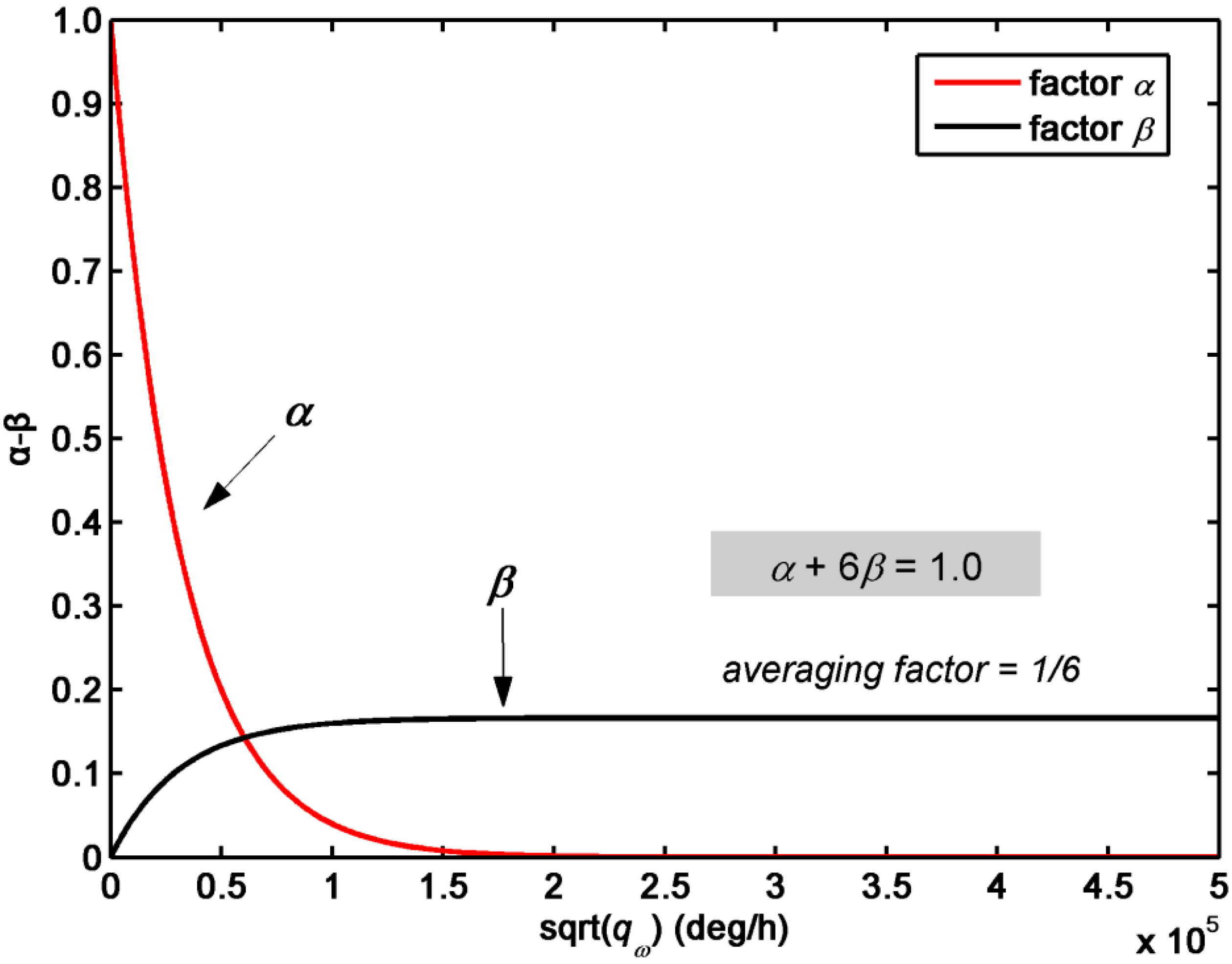 will dominate the values of compared to the ZK+1. In this case, the performance of KF is higher than that of an averaging process. The factor α will converge to zero and β will approach an averaging effect factor of 1/6 with increasing values of qω, at this point the output of the KF entirely depends on the measurements of ZK+1, and it is approximately equal to the effect of an averaging process. Therefore, by analyzing the KF weight factor, the KF dependency on the estimated value and measurement value ZK+1 can be observed directly. Meanwhile, the relationship between the performance of KF and a simple averaging process is revealed, providing a basis for choosing the system designing parameters.
3.2. Analysis of Sampling and Filtering Rate on Accuracy Improvement
 , thus the discrete-time model for describing the true angular rate signal can be expressed as:
 due to the F = 0. Thus, according to the Equation (12), the KF filtering model of Equations (6) and (10) will be more accurate when the input rate signal is nearly zero or with a constant characteristic, in such a situation, a considerable accuracy improvement can be obtained by the KF. On the contrary, the accuracy improvement would be degraded due to an inexact filtering model when the input rate signals have a high dynamic characteristic, because the variations between the values of the two input rate signals associated with the adjacent time points increase in a high dynamic condition, while the KF model requires a smaller variations. To overcome this problem, the sensors sampling rate and KF filtering rate can be increased to reduce the variations between the values of two input rate signals. In the simulation sections, the influence of the sensors sampling rate and KF filtering rate on accuracy improvement will be analyzed and evaluated.
4. Dynamic Simulation of Virtual Gyroscope

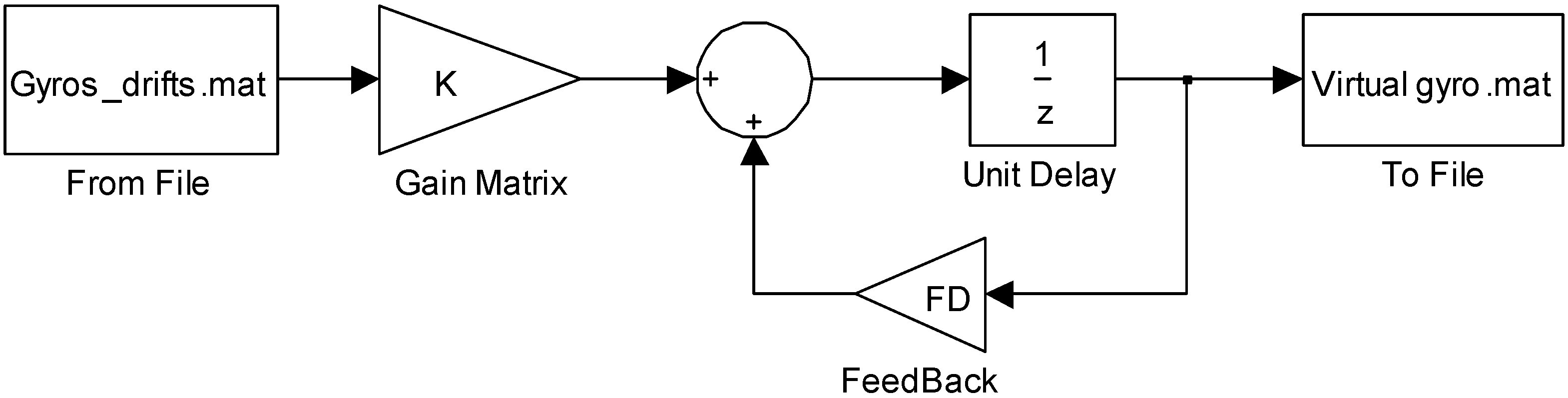
 is the estimate of the true angular rate associated with the ith time, and ωi,true is the true angular rate associated with the ith time, and n is the length number of samples. The simulink model for discrete-time KF (Equation (10)) is shown as Figure 2.
4.1. Influence of Signal Frequency on Dynamic Performance Improvement
. After the peak, the IF begins to decline and eventually reaches the steady-state value. There exists a peak corresponding to the maximum IF during the whole range of parameter qω under a frequency f. Consequently, in this work, based on the multiple simulations, we analyze the influence of frequency f on the KF dynamic performance improvement, where f is the frequency of the input swing rate signal. It can be concluded that the maximum improvement factor can be determined and achieved for a dynamic input rate signal having a frequency of f. It can also be found that the maximum improvement factor is different with the various frequency f of the input rate signal. Thus, the relationship between the maximum improvement factor and input signal frequency f will be analyzed.. The true angular rate signal is assumed to be a swing input signal ω = A·sin(2πft), with an amplitude of A = 5 and 10°/s, respectively. The frequency f is chosen to be in the range from 0 to 10 Hz. The maximum improvement factor versus frequency f is plotted in Figure 3. Note that a specific value of qω corresponds to each frequency in Figure 3, by choosing such values, the maximum improvement factor can be obtained, i.e., the optimal qω varies with f.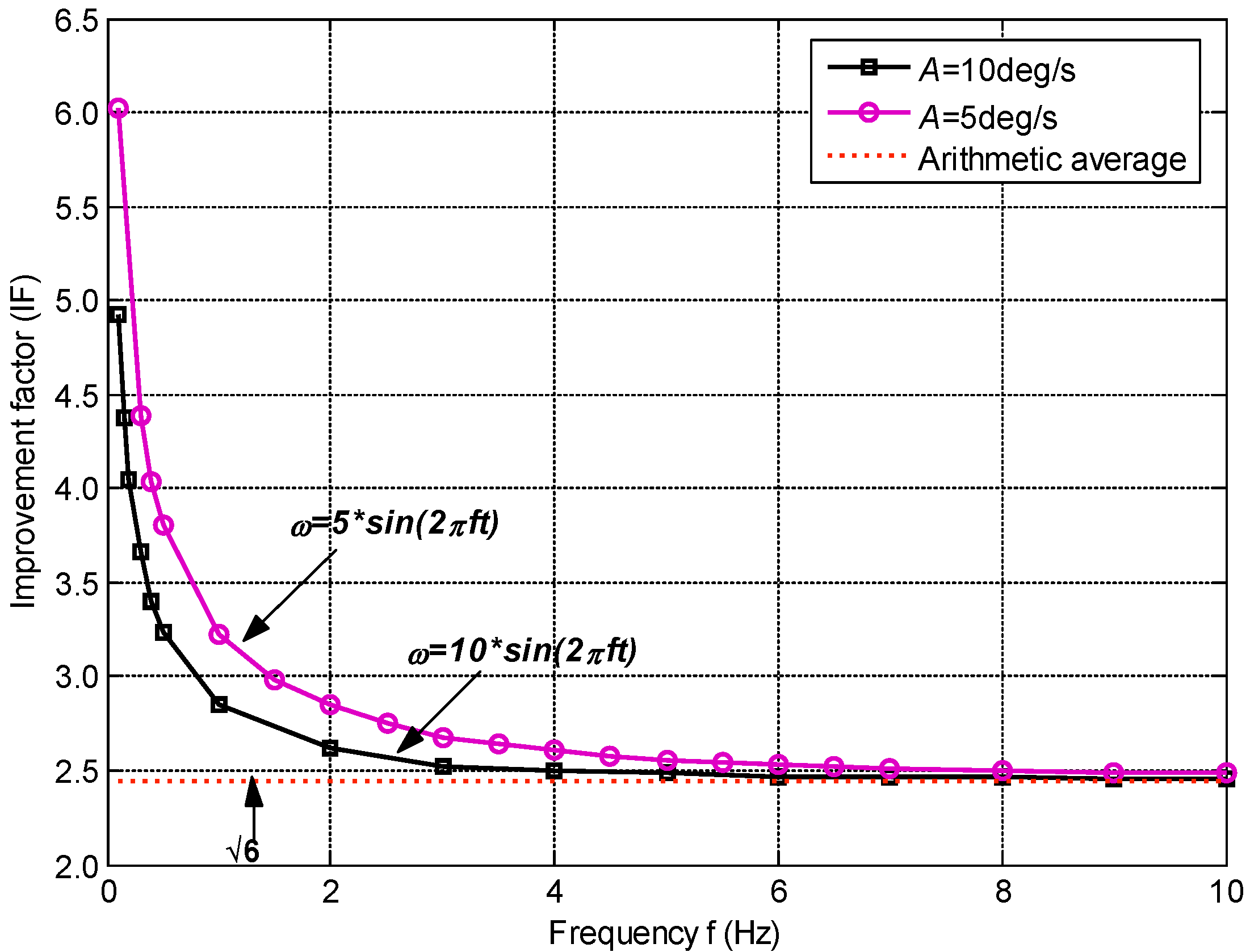
 . The graph also shows that the improvement factor is higher than for the frequency f range from 0 to 10 Hz. In addition, it displays a greater slope of the improvement factor for lower input frequencies (0 to 3 Hz) than for higher frequency. Furthermore, the improvement factor obtained by a smaller amplitude (A = 5°/s) is higher than that of the input rate signal with a larger amplitude, this is because the signal’s dynamic property is determined by both of the amplitude and frequency.
4.2. Influence of Sampling and Filtering Rate on Accuracy Improvement
. The input rate signal is assumed to be a sinusoidal signal of ω = A·sin(2πft) with the amplitude A = 30°/s and frequency f = 10 Hz. Three different KF filtering rates are chosen, i.e., fKF = 500, 250, and 100 Hz. For the filtering rate fKF = 250 and 100 Hz, there exist two methods for processing the raw data: (1) Interval average filtering, i.e., calculating the arithmetic average of the input rate signal contained in a filtering period, and then regarding the averaged rate signals as a new measurement sequence for KF processing; (2) Interval sampling filtering, i.e., selecting one of the input rate signals in a filtering period as the new measurement sequences for KF processing. Using the simulink model (Figure 2), the outputs of virtual gyroscope are shown in Figure 4. The detailed results are illustrated in Table 1. for two different processing methods with filtering rates of fKF = 500, 250, 100 Hz. (a) Interval average filtering. (b) Interval sampling filtering.
for two different processing methods with filtering rates of fKF = 500, 250, 100 Hz. (a) Interval average filtering. (b) Interval sampling filtering.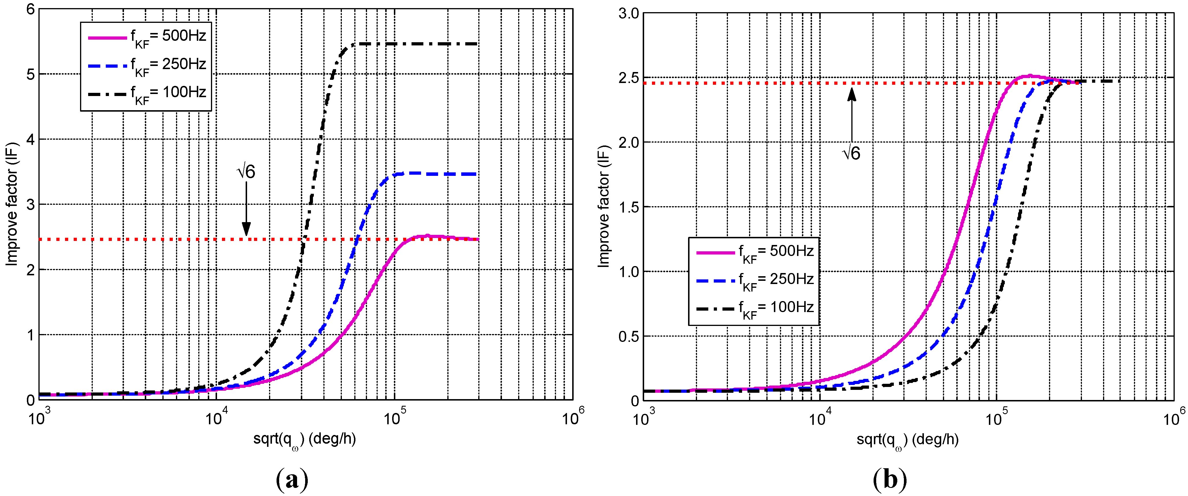

| Terms | 500 Hz | Interval average filtering | Interval sampling filtering | ||
|---|---|---|---|---|---|
| 250 Hz | 100 Hz | 250 Hz | 100 Hz | ||
| Optimal (°/h) | 154,900 | 123,100 | 76,000 | 214,300 | 295,200 |
| Estimated error (1σ, °/s) | 0.5946 | 0.4301 | 0.2730 | 0.6044 | 0.6044 |
| Maximum improvement factor ( IF) | 2.6037 | 3.4669 | 5.4612 | 2.4670 | 2.4670 |
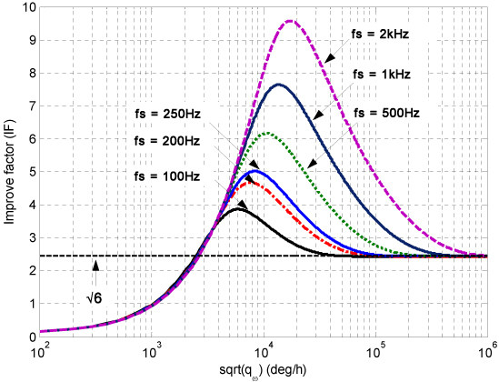
 , where m is the number of rate signals that were contained in a filtering period. However, the method of the interval average filtering is not suitable for application having a larger dynamic characteristic. It may result in an inaccuracy of measurements for KF due to the average process, and this inaccuracy will increase with increasing numbers of rate signals in a filtering period. As for the method of interval sampling filtering, the maximum IF associated with the filtering rate 250 Hz is 2.467, which is lower than that of 500 Hz, namely 2.6037. The reason lies in that the variations between the values of two input rate signals associated with adjacent time points are increased through interval sampling, resulting in a larger model error than that of the filtering rate fKF = 500 Hz, and eventually degrading the KF performance. Therefore, the KF filtering rate should be set to be the same as the sensors sampling rate to reduce the estimated error. is obtained as shown in Figure 5. The detailed results are shown in Table 2. with larger values of , i.e., the averaging effect. Table 2 indicates that the 1σ error is reduced from 2.9893°/s to 0.7715°/s when the fs = 100 Hz, which is larger than the result of 0.2738°/s corresponding to the sampling rate 3 kHz. This is because the amplitude variation between the two signals for the adjacent time point becomes smaller with increasing sampling rate, implying that the KF model error is decreased. In addition, the plot also illustrates that the optimal range for located in which the IF is higher than will be magnified with increasing fs. under different sampling rates fs = 100, 200, 250, 500, 1000, 2000, 3000 Hz.
under different sampling rates fs = 100, 200, 250, 500, 1000, 2000, 3000 Hz.
, where m is the number of rate signals that were contained in a filtering period. However, the method of the interval average filtering is not suitable for application having a larger dynamic characteristic. It may result in an inaccuracy of measurements for KF due to the average process, and this inaccuracy will increase with increasing numbers of rate signals in a filtering period. As for the method of interval sampling filtering, the maximum IF associated with the filtering rate 250 Hz is 2.467, which is lower than that of 500 Hz, namely 2.6037. The reason lies in that the variations between the values of two input rate signals associated with adjacent time points are increased through interval sampling, resulting in a larger model error than that of the filtering rate fKF = 500 Hz, and eventually degrading the KF performance. Therefore, the KF filtering rate should be set to be the same as the sensors sampling rate to reduce the estimated error. is obtained as shown in Figure 5. The detailed results are shown in Table 2. with larger values of , i.e., the averaging effect. Table 2 indicates that the 1σ error is reduced from 2.9893°/s to 0.7715°/s when the fs = 100 Hz, which is larger than the result of 0.2738°/s corresponding to the sampling rate 3 kHz. This is because the amplitude variation between the two signals for the adjacent time point becomes smaller with increasing sampling rate, implying that the KF model error is decreased. In addition, the plot also illustrates that the optimal range for located in which the IF is higher than will be magnified with increasing fs. under different sampling rates fs = 100, 200, 250, 500, 1000, 2000, 3000 Hz.
under different sampling rates fs = 100, 200, 250, 500, 1000, 2000, 3000 Hz.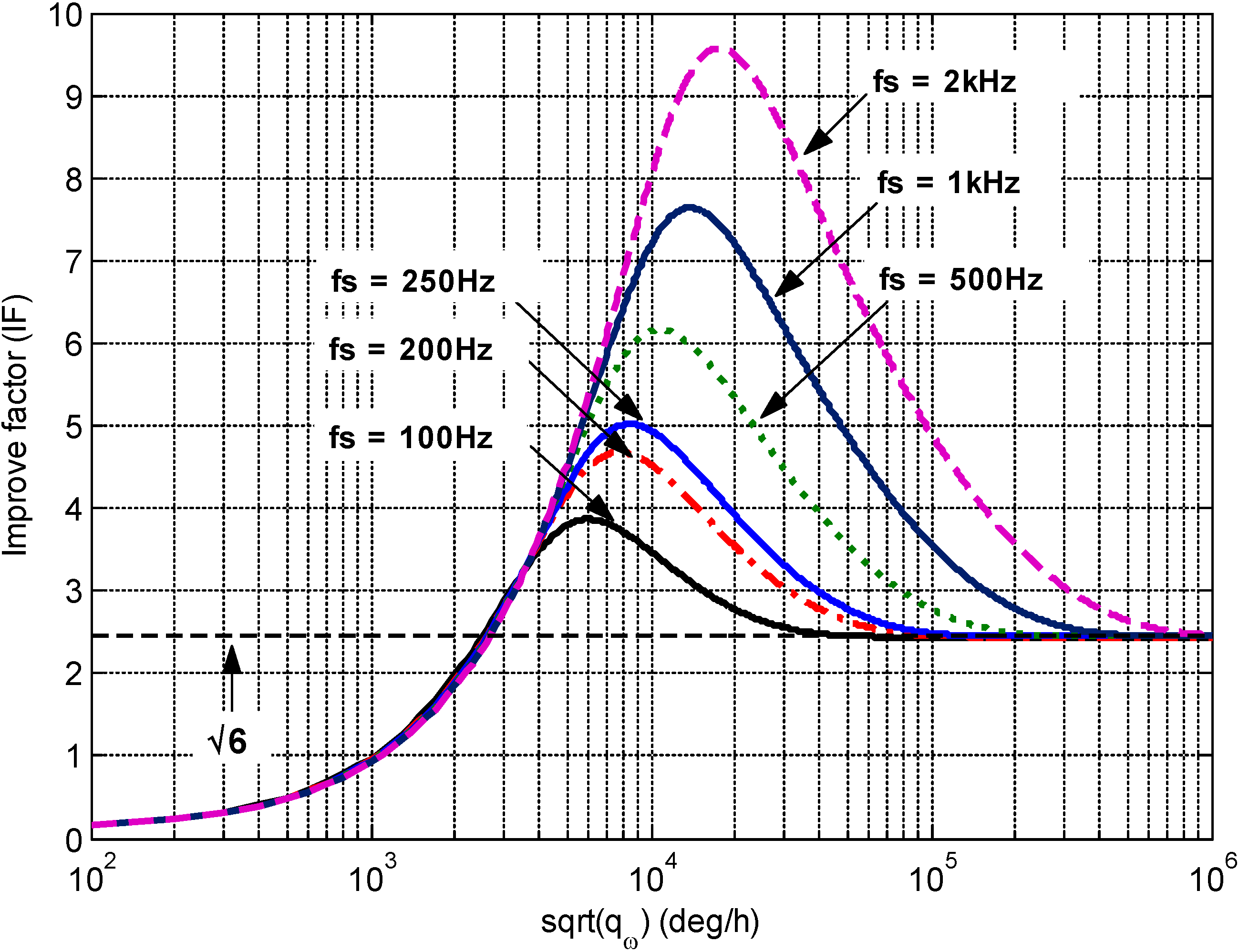
| Sampling rate fs (Hz) | Estimated error 1σ (°/s) | Maximum improvement factor | |
|---|---|---|---|
| Single gyro | Virtual gyro | ||
| 100 | 2.9839 | 0.7715 | 3.8677 |
| 200 | 2.9837 | 0.6380 | 4.6766 |
| 250 | 2.9813 | 0.5941 | 5.0182 |
| 500 | 2.9812 | 0.4836 | 6.1646 |
| 1000 | 2.9807 | 0.3903 | 7.6369 |
| 2000 | 2.9820 | 0.3116 | 9.5700 |
| 3000 | 2.9802 | 0.2738 | 10.8846 |

5. Experiments

| Term | Gyro1 | Gyro2 | Gyro3 | Gyro4 | Gyro5 | Gyro6 |
|---|---|---|---|---|---|---|
| ARW (°/ ) | 6.3032 | 6.2308 | 6.2308 | 6.3382 | 6.2845 | 6.2555 |
| Bias Instability (°/h) | 59.2476 | 58.3598 | 60.3401 | 60.1159 | 57.7861 | 60.0119 |
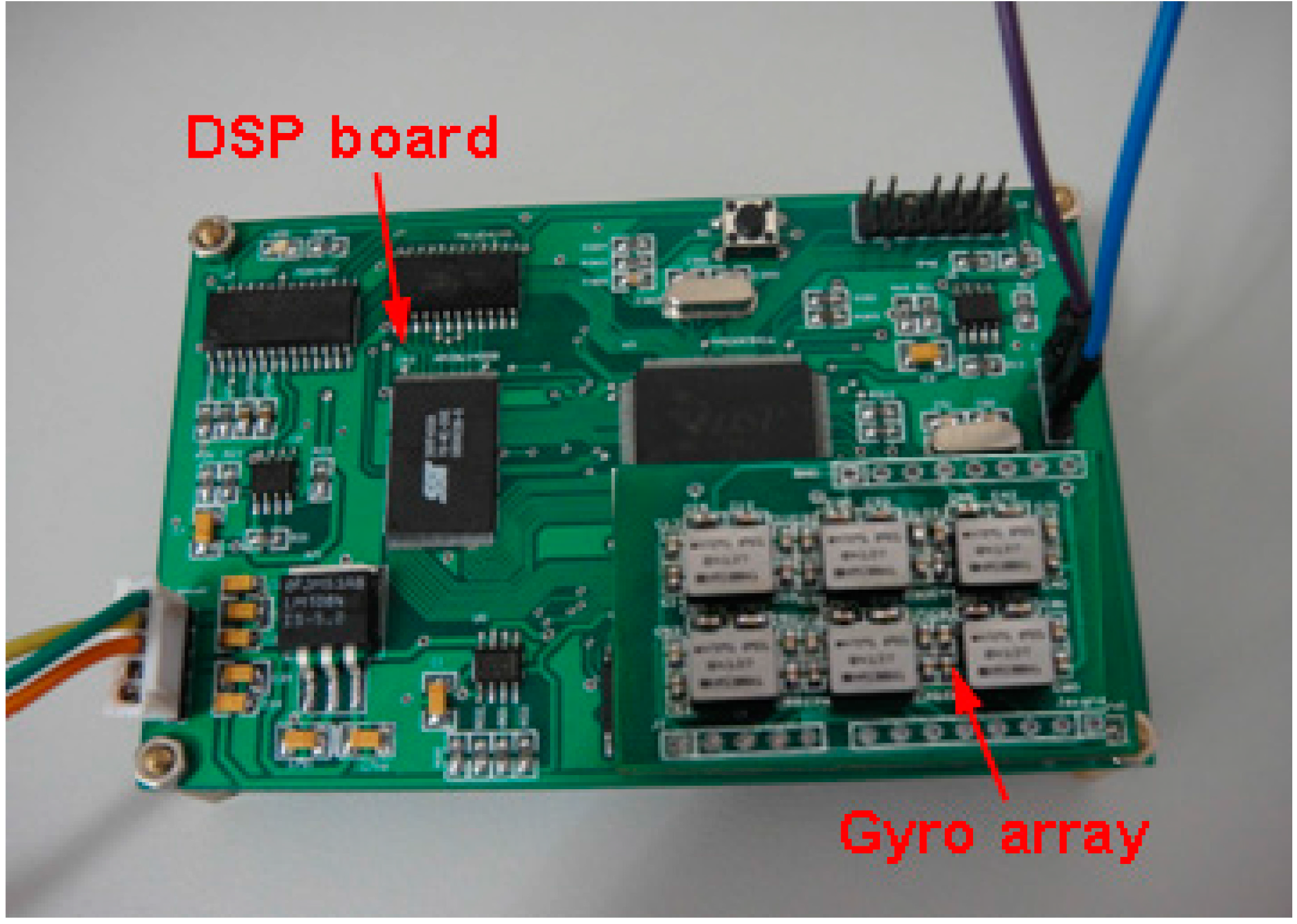
 and C are single variables. Hence, the system computation is mainly dependent on the matrix operation of HTR−1Zk+1. Furthermore, the number of N and noise statistics of the gyroscopes will be determined and fixed while the sensors array is determined. At this time, the covariance matrix R can be determined. Therefore, the value of parameter and matrix
  can be calculated off-line in advance, and then these parameters can be written into the program for real-time processing of the information coming from the sensors array, in which case the computational burden becomes a matrix product with the matrix dimensioned of 1 × N multiplied by the matrix dimensioned of N × 1, with computational complexity of only O(N). Thus, a DSP processor could completely satisfy the system requirements of real-time processing.
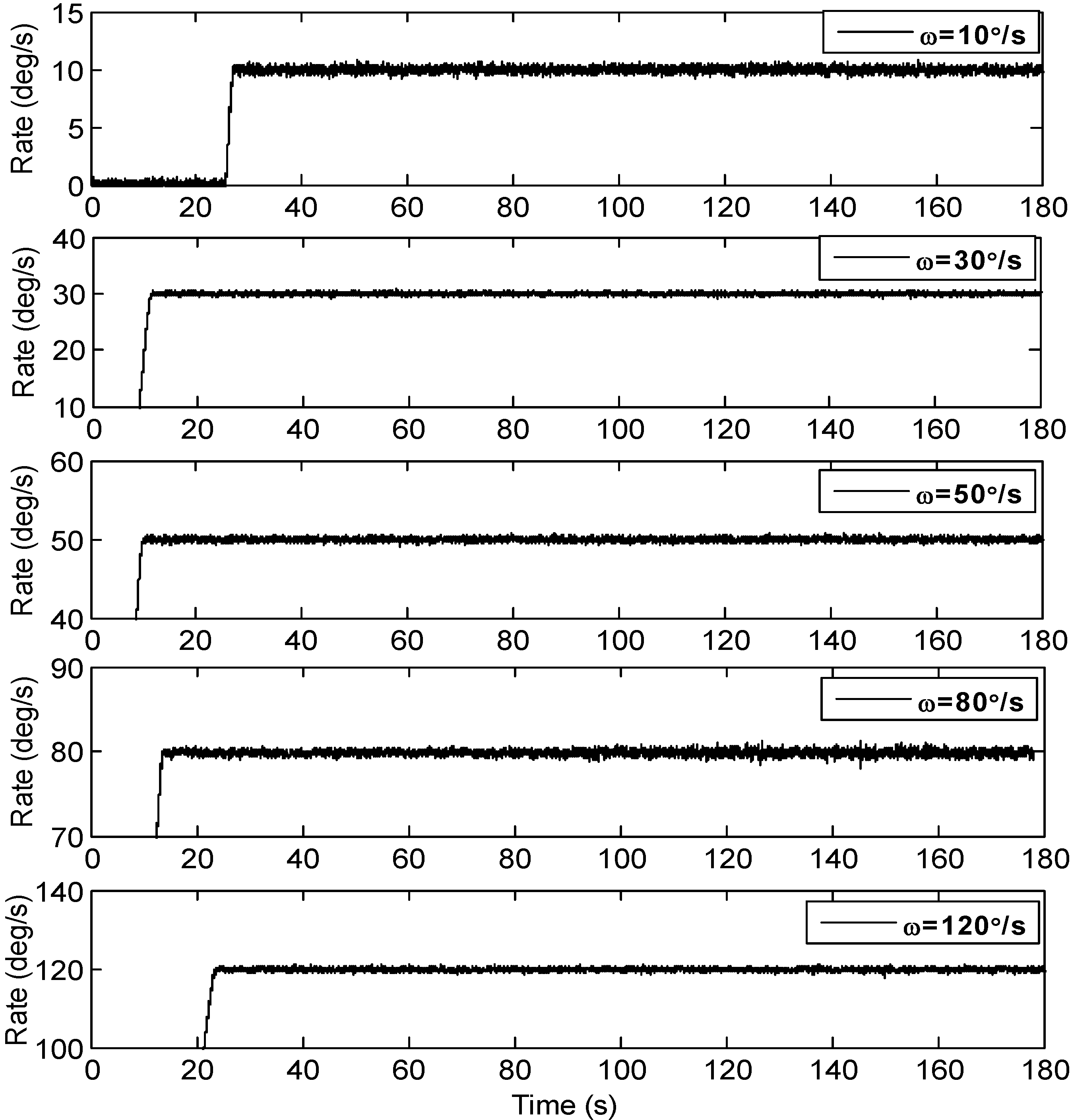
5.1. Constant Rate Signal Test

| Input rate ω (°/s) | Estimated error 1σ (°/s) | Improvement factor IF | |
|---|---|---|---|
| Single gyro | Virtual gyro | ||
| 10 | 2.0094 | 0.2027 | 9.9132 |
| 30 | 2.0189 | 0.2015 | 10.0194 |
| 50 | 2.0391 | 0.2063 | 9.8841 |
| 80 | 2.5253 | 0.2743 | 9.2063 |
| 120 | 2.9225 | 0.3395 | 8.6082 |
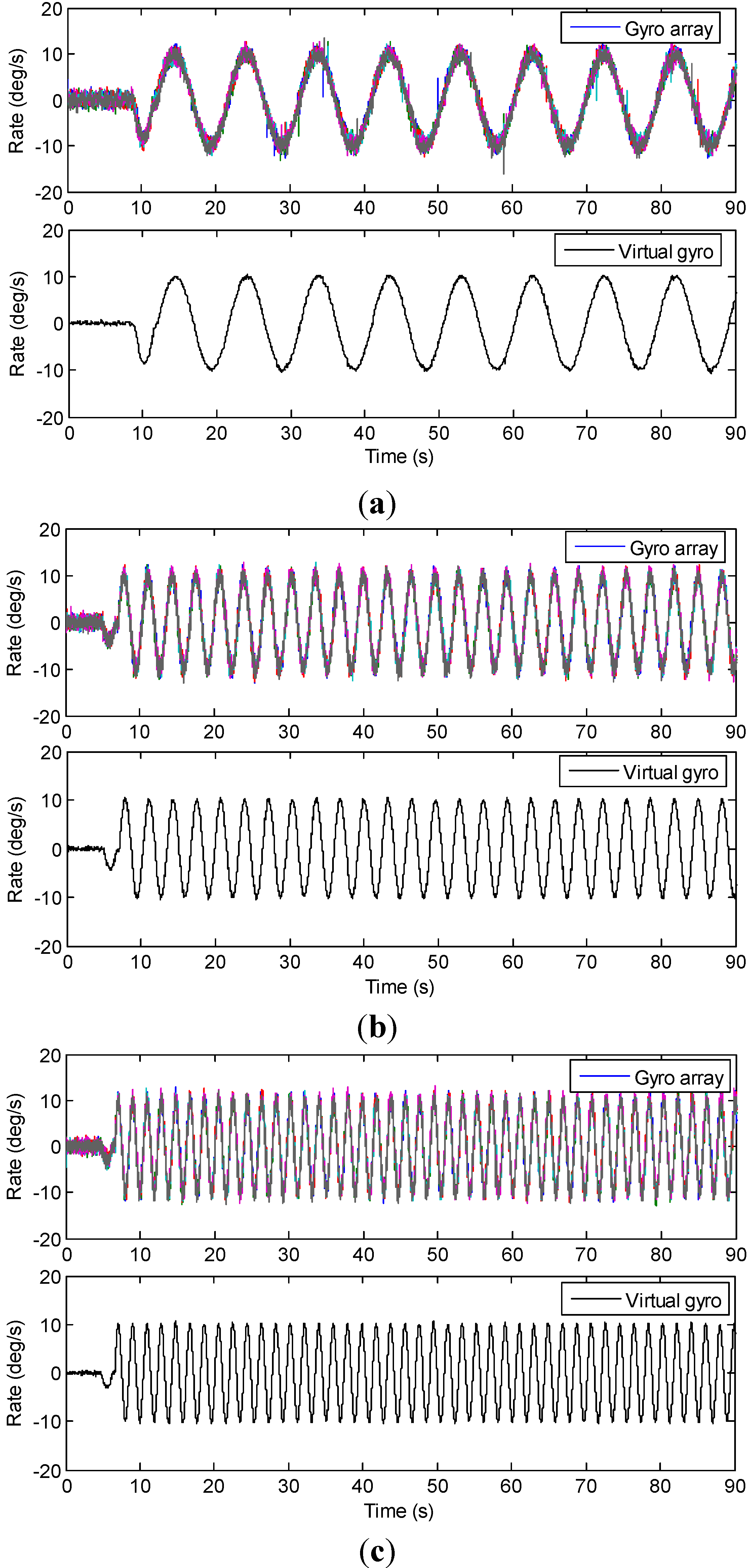
5.2. Swing Rate Signal Test
| Frequency f (Hz) | Single gyro (°/s) | Virtual gyro (°/s) | Improvement factor ( IF) | ||||
|---|---|---|---|---|---|---|---|
| amplitude | 1σ error | amplitude | 1σ error | experiment | simulation | error (%) | |
| 0.1 | 12.4463 | 1.5724 | 10.5238 | 0.3023 | 5.2015 | 4.9252 | 5.6099 |
| 0.3 | 12.5270 | 1.6121 | 10.6258 | 0.4767 | 3.3818 | 3.6660 | 7.7523 |
| 0.5 | 12.6268 | 1.6954 | 10.6293 | 0.4858 | 3.4899 | 3.2357 | 7.8561 |

6. Conclusions
Acknowledgments
Author Contributions
Conflicts of Interest
References
- Guo, Z.Y.; Lin, L.T.; Zhao, Q.C.; Cui, J.; Chi, X.Z.; Yang, Z.C.; Yan, G.Z. An electrically decoupled lateral-axis tuning fork gyroscope operating at atmospheric pressure. In Proceedings of the IEEE 22nd International Conference on Micro Electro Mechanical Systems, Sorrento, Italy, 25–29 January 2009; pp. 104–107.
- Yazdi, N.; Ayazi, F.; Najafi, K. Micromachined inertial sensors. Proc. IEEE 1998, 86, 1640–1659. [Google Scholar]
- Nitzan, S.; Ahn, C.H.; Su, T.-H.; Li, M.; Ng, E.J.; Wang, S.; Yang, Z.M.; O’Brien, G.; Boser, B.E.; Kenny, T.W.; Horsley, D.A. Epitaxially-encapsulated polysilicon disk resonator gyroscope. In Proceedings of the IEEE 26th International Conference on Micro Electro Mechanical Systems, Taipei, Taiwan, 20–24 January 2013; pp. 625–628.
- Pakniyat, A.; Salarieh, H. A parametric study on design of a microrate-gyroscope with parametric resonance. Measurement 2013, 46, 2661–2671. [Google Scholar] [CrossRef]
- Mariani, S.; Ghisi, A.; Corigliano, A.; Martini, R.; Simoni, B. Two-scale simulation of drop-induced failure of polysilicon MEMS sensors. Sensors 2011, 11, 4972–4989. [Google Scholar] [CrossRef]
- Sonmezoglu, S.; Alper, S.E.; Akin, T. An automatically mode-matched MEMS gyroscope with 50 Hz bandwidth. In Proceedings of the IEEE 25th International Conference on Micro Electro Mechanical Systems, Paris, France, 29 January–2 February 2012; pp. 523–526.
- Wang, W.; Lv, X.; Sun, F. Design of a novel MEMS gyroscope array. Sensors 2013, 13, 1651–1663. [Google Scholar] [CrossRef]
- Kim, S.; Chun, K. A gyroscope array with capacitive detection. J. Korean Phys. Soc. 2002, 40, 595–600. [Google Scholar] [CrossRef]
- Tanenhaus, M.; Carhoun, D.; Geis, T.; Wan, E.; Holland, A. Miniature IMU/INS with optimally fused low drift MEMS gyro and accelerometers for applications in GPS-denied environments. In Proceedings of IEEE Symposium on Position, Location and Navigation, Myrtle Beach, SC, USA, 23–26 April 2012; pp. 259–264.
- Al-Majed, M.I.; Alsuwaidan, B.N. A new testing platform for attitude determination and control subsystems: Design and applications. In Proceedings of the IEEE/ASME International Conference on Advanced Intelligent Mechatronics, Singapore, Singapore, 14–17 July 2009; pp. 1318–1323.
- Bayard, D.S.; Ploen, S.R. High accuracy inertial sensors from inexpensive components. U.S. Patent US20030187623A1, 2 October 2003. [Google Scholar]
- Chang, H.; Xue, L.; Qin, W.; Yuan, G.; Yuan, W. An integrated MEMS gyroscope array with higher accuracy output. Sensors 2008, 8, 2886–2899. [Google Scholar] [CrossRef]
- Xue, L.; Jiang, C.Y.; Chang, H.L.; Yang, Y.; Qin, W.; Yuan, W.Z. A novel Kalman filter for combining outputs of MEMS gyroscope array. Measurement 2012, 45, 745–754. [Google Scholar] [CrossRef]
- Chang, H.L.; Xue, L.; Jiang, C.Y.; Kraft, M.; Yuan, W.Z. Combining numerous uncorrelated MEMS gyroscopes for accuracy improvement based on an optimal Kalman filter. IEEE Trans. Instrum. Meas. 2012, 61, 3084–3093. [Google Scholar] [CrossRef]
- Colomina, I.; Giménez, M.; Rosales, J.J.; Wis, M.; Gomez, A.; Miguelsanz, P. Redundant IMUs for precise trajectory determination. In Proceedings of the 20th ISPRS Congress, Istanbul, Turkey, 12–23 July 2004; pp. 1–7.
- Waegli, A.; Skaloud, J.; Guerrier, S.; Parés, M.E.; Colomina, I. Noise reduction and estimation in multiple micro-electro-mechanical inertial systems. Meas. Sci. Technol. 2010, 21, 065201. [Google Scholar] [CrossRef]
- Wis, M.; Colomina, I. Dynamic dependent IMU stochastic modeling for enhanced INS/GNSS navigation. In Proceedings of the 5th ESA Workshop on Satellite Navigation Technologies and European Workshop on GNSS Signals and Signal Processing, Noordwijk, The Netherlands, 8–10 December 2010; pp. 1–5.
- Stebler, Y.; Guerrier, S.; Skaloud, J.; Victoria-Feser, M.-P. The generalized method of wavelet moments for inertial navigation filter design. IEEE Trans. Aerosp. Electron. Syst. 2012, 2012, 24193. [Google Scholar]
- Sadaghzadeh-Nokhodberiz, N.; Poshtan, J.; Wagner, A.; Nordheimer, E.; Badreddin, E. Cascaded Kalman and particle filters for photogrammetry based gyroscope drift and robot attitude estimation. ISA Trans. 2014, 53, 524–532. [Google Scholar] [CrossRef]
- El-Sheimy, N.; Hou, H.; Niu, X. Analysis and modeling of inertial sensors using Allan variance. IEEE Trans. Instrum. Meas. 2008, 57, 140–149. [Google Scholar] [CrossRef]
- Analog devices, ADXRS300. Available online: http://www.analog.com/static/imported-files/data_sheets/ADXRS300.pdf (accessed on 4 November 2014).
- Texas Instrum, TMS320VC5416. Available online: http://focus.ti.com/docs/prod/folders/print/tms320vc5416.html (accessed on 4 November 2014).
- Burr-Brown Products from Texas Instruments, ADS7807. Available online: http://focus.ti.com/lit/ds/symlink/ads7807.pdf (accessed on 4 November 2014).
- Guerrier, S.; Skaloud, J.; Stebler, Y.; Victoria-Feser, M.-P. Wavelet variance based estimation for composite stochastic processes. J. Am. Stat. Assoc. 2013, 108, 1021–1030. [Google Scholar] [CrossRef]
© 2014 by the authors; licensee MDPI, Basel, Switzerland. This article is an open access article distributed under the terms and conditions of the Creative Commons Attribution license (http://creativecommons.org/licenses/by/4.0/).
Share and Cite
Xue, L.; Wang, L.; Xiong, T.; Jiang, C.; Yuan, W. Analysis of Dynamic Performance of a Kalman Filter for Combining Multiple MEMS Gyroscopes. Micromachines 2014, 5, 1034-1050. https://doi.org/10.3390/mi5041034
Xue L, Wang L, Xiong T, Jiang C, Yuan W. Analysis of Dynamic Performance of a Kalman Filter for Combining Multiple MEMS Gyroscopes. Micromachines. 2014; 5(4):1034-1050. https://doi.org/10.3390/mi5041034
Chicago/Turabian StyleXue, Liang, Lixin Wang, Tao Xiong, Chengyu Jiang, and Weizheng Yuan. 2014. "Analysis of Dynamic Performance of a Kalman Filter for Combining Multiple MEMS Gyroscopes" Micromachines 5, no. 4: 1034-1050. https://doi.org/10.3390/mi5041034
APA StyleXue, L., Wang, L., Xiong, T., Jiang, C., & Yuan, W. (2014). Analysis of Dynamic Performance of a Kalman Filter for Combining Multiple MEMS Gyroscopes. Micromachines, 5(4), 1034-1050. https://doi.org/10.3390/mi5041034