1. Introduction
During the last twenty years, microfluidic devices have been developed for a broad range of applications in bio-analysis and chemical processing technologies. The original fabrication techniques of the microfluidic devices were derived from the semiconductor industry and most devices adopted silicon or glass as the substrates. These techniques were thought to be intricate and expensive. In recently years, polymeric materials have been extensively used for the fabrication of the microfluidic devices. Among these materials, poly(dimethylsiloxane) (PDMS) receives a lot of attention due to its optical transparency and biocompatibility and is utilized as the main substrate for various microfluidic systems.
Liquid filling is commonly encountered in the operation of the microfluidic chip. Chips utilize lengthy microchannels to deliver liquid solution or air bubbles in liquids from one place to another or bring different liquid fluids into microchambers [
1]. Before using the microfluidic chips, the channels are usually washed via flushing through water or solvent, and then dried by hot air. When used, the inlet of the chip is connected with a larger buffer liquid reservoir. The driving forces accompanied with surface tension will pull the liquid into the microchannels. Sometimes surface tension may be the sole driving force to help the liquid flow into the chip.
Pressure, high electric fields and gravity are usually exploited to drive the flow of liquid in microchannels. However, surface tension, which is typically negligible in macro-scale systems, is also a force responsible for a variety of physical phenomena involving small volumes of liquid. Molecules in the liquid state exert strong attractive forces on each other. Surface tension, a cohesive force, arises from attractive forces among the molecules in a fluid, whereas an adhesive force to the wall acts on the fluid interface at the contact point with the wall. Yang
et al. [
2] used the marching velocity or position of the meniscus front, which was driven by the capillary force and the gravitational effect, to measure the surface energy inside a parylene microchannel. They proposed a one-dimensional mathematical model to evaluate the liquid-filling behavior in a straight microchannel. Kung
et al. [
3] demonstrated the balance among the inertial, surface tension, gravitational, and frictional forces of blood flow characteristics in a glass microchannel. Trung
et al. [
4] used compressed air and air-sucking to load the PCR sample into the microfluidic chip. The loading rate of the sample results from the competition between the air pressure and the surface tension. They examined the dependence of the loading rate of a PCR mixture on the thickness of the PDMS wall between the reaction chamber and the air jacket. The surface tension dominates the autonomous fluid movement in a hydrophilic microchannel, e.g., glass or poly(methyl methacrylate) (PMMA) channels. However, because of the intrinsic hydrophobicity of PDMS or parylene, it is difficult to move fluid in a hydrophobic microchannel using only surface tension force.
The advantages of utilizing the surface tension effect in microsystems include lower power consumption, ease of fabrication and no active fluidic component. A variety of applications for surface tension exist in microelectromechanical systems (MEMS), including hydrophobic valves [
5], micro-injection molding [
6], flow switches [
7], liquid metering [
8], surface tension-powered self assembly [
9], microstructure formation [
10], ink-jet printing [
11], plasma extraction [
12], and cell culture [
13].
Experimental and numerical studies of surface tension-driven flow in microchannels have been performed. Tseng
et al. [
14] studied the process of a liquid slug, which was blown by an air flow moving in and out of the micro reservoir. They used the volume-of-fluid (VOF) method as a numerical scheme and considered surface tension as a volumetric force. Results showed that the success of reservoir-filling strongly depends on the designs of the hydrophilic wall surface and the wall shape/size of the flow network. Leu and Chang [
15] presented the capillary stop valves and micro sample separator, which were using a pressure barrier. The pressure barrier of the stop valve design could be predicted well by utilizing the three-dimensional meniscus method. Jensen
et al. [
16] examined the quasi-static motion of wetting bubbles in microchannel contractions. The entire system close to equilibrium for all bubble positions was assumed. Based on their analysis, they established three design rules for reducing the pressure that is needed to push the bubbles out of the contraction. Chen
et al. [
17] examined the surface tension flow of open microchannels with turning angles from 45° to 135°. It is shown that the turning angle plays a major role in the meniscus of liquid-gas interface shape.
The simulation of surface tension-driven flow in microchannels has been attracting a lot of attention. Results were generated by assuming a constant value of the contact angle, which means that only the static contact angles were applied in all previous computational research. The contact angle is the angle between the free liquid surface and the confining wall, and is a result of the competition between surface tension and the adhesive force. When the competing forces are in balance, the contact line,
i.e., the line where a solid meets the liquid-gas interface, does not move and the matching contact angle is then called static. If the forces are out of balance, the contact line will move towards its equilibrium position creating a dynamic contact angle. The velocity with which the contact line moves is called the contact line velocity and is often modeled as a function of the dynamic contact angle [
18,
19]. However, the static contact angle was still utilized to consider the moving meniscus qualitatively to deduce some filling strategies in recent studies.
In numerical treatment of moving contact lines, contact angles are required and applied as a boundary condition at the contact line. However, the dynamic contact angle of the contact line depends on the velocity of the moving contact line. A mean-field free-energy lattice Boltzmann model was used to solve the moving contact line problem of liquid-vapor interfaces and the dynamics of the wetting and movement of a three-phase contact line confined between two superhydrophobic surfaces [
20,
21]. The velocity fields near the interface were in good agreement with fluid mechanics and molecular dynamics studies. The dynamic contact angle in a microchannel could be larger (advancing) or smaller (receding) than the static contact angle [
22]. In all of the aforementioned studies, the effects of the relationship between the contact angle and the contact line velocity on the flow characteristics inside the microchannel or microchamber were not investigated. A computational model with a simplified linear relationship between the contact angle and the contact line velocity has been utilized in previous studies. Baer
et al. [
23] developed a finite element moving mesh model in two sample problems: solid body rotation of a fluid and extrusion from a nozzle with a rectangular cross-section. Šikalo
et al. [
24] studied the drop impact using a volume-of-fluid based method. The predicted time dependence of the drop-spreading diameter and of the dynamic contact angle agrees well with the experimental data for both the advancing and receding phases of the impact process. Afkhami and Bussmann utilized [
25,
26] three models of contact angle variation with contact angle velocity on predictions of drop impact. The linear relationship between the contact angle and the contact line velocity is simple and can predict well the change of the dynamic contact angle. In our study, a generalized form with velocity-dependent contact angles is implemented for the calculation of surface tension forces in a volume-of-fluid based model.
Understanding the liquid filling process is significant to design microfluidic chips. Successful filling by the liquid flows of microchannels or microchambers is not as easy as that of a macro-scale system because the surface effects are significant [
7]. Different geometry of microchannels or microchambers may result in different filling behavior such as filling time or the possibility of entrapping an air bubble,
etc. If the chip is poorly designed, then air may easily become entrapped in the micro cavities, degrading the functions of the systems. In our previous study [
27], the entrapment of air bubbles in the oval disk-shaped chamber as a free surface moved through the microstructure during the filling process was examined. The two-dimensional numerical results indicated linear relationships between the formation of the bubble and both the Weber number and the sum of the static contact angle and the change in the angle between the microchannels and the microchamber at the intersection. However, the flow front shapes differed between numerical simulations and experimental interface locations, especially in regions in which the flow front entered the chamber after it passed around a sharp corner. Therefore, understanding the effects of surface tension, adhesion and inertia on fluid flows with dynamic contact angles in microchannels or microchambers is of marked importance in the related fields of science, medicine and engineering.
This work numerically establishes the filling processes of the liquid in the disk-shaped microstructures by considering microchambers with inlets and outlets fabricated using MEMS technologies. Three-dimensional governing equations are adopted to simulate the fluid flows inside the microfluidic devices. A general functional form with velocity-dependent contact angles is implemented for the accurate calculation of surface tension forces in a volume-of-fluid based model. The effects of the parameters of the functional form are investigated. Finally, the microfluidic devices are fabricated in PDMS substrates simply from a mold. Due to the hydrophobicity of the PDMS, the oxygen plasma treatment method is used to modify the surface of PDMS microchannels to be hydrophilic. Flow experiments are conducted into both hydrophilic and hydrophobic PDMS microstructures and the results compared with those of numerical simulations.
2. Mathematical Model and Numerical Methodology
The liquid filling processes inside an oval or a circular disk-shaped microchamber are accepted to be governed by the continuity and the Navier-Stokes equations subject to appropriate boundary and initial conditions. Numerical simulations are conducted to elucidate the motion of a liquid flow inside the microchannels and the oval disk-shaped microchamber.
Assuming that the fluid obeys the linear Newtonian friction law and neglecting the compressibility, the governing equations comprise conservation of mass and momentum, and a scale function, F, of the liquid volume fraction inside a computational cell. The conservation equations of mass and momentum are solved to yield the motion and the shape of the gas-liquid interface. The continuity equation can be expressed as follows:
where
![Micromachines 05 00116 i008]()
is the fluid velocity vector.
The momentum equation for a continuum is the analogue of Newton’s second law for a point mass. The momentum principle states that the rate of change of linear momentum of material in a region equals the sum of the forces on that region. Two such forces may be included: body forces, which act on the bulk of the material in the region, and surface forces, which act on the boundary surface. The momentum equation,
i.e., the Navier Stokes Equation, is
where
t is time,
ρ is the fluid density,
P is the static pressure, and
v is the kinematic viscosity of the fluid. The last term on the right hand side of Equation (2) is the volumetric surface tension, which can be calculated using the continuum surface force (CSF) model. Surface tension-driven flows are source-term dominated, and convergent solutions become difficult to obtain numerically.
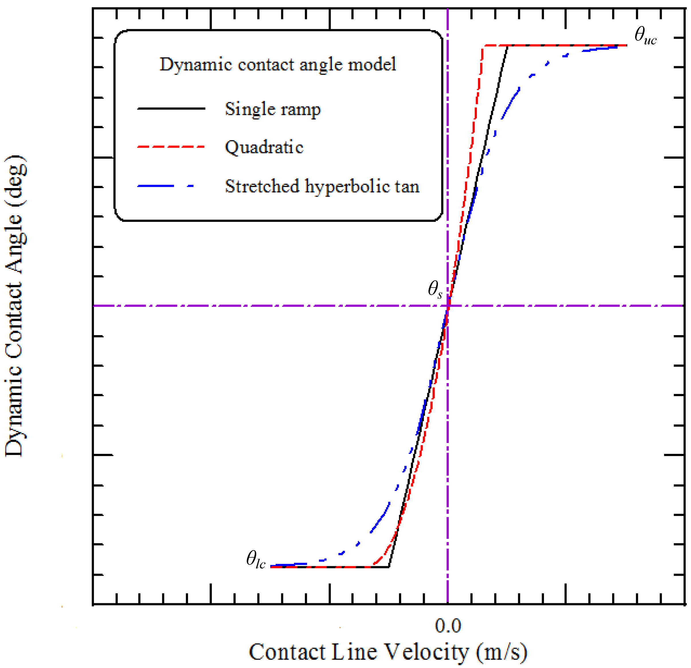
The orientation of the interface near the contact line reflects the contact angle, which is the angle between the normal to the liquid-solid interface and the normal to the solid surface at the contact line. A general correlation for the contact angle as a function of contact line velocity is not easy to be obtained. van Mourik
et al. [
18] gave a brief summary about the contact angles models. The theoretical studies on the dynamic contact angle carried out in the last few decades have led to numerous theoretical dynamic contact angle models. In contrast with the theoretical analyses, dynamic contact angle models have also been proposed based on experimental measurements. The Blake’s model [
28,
29], which is based on molecular kinetics, is one of the most common used dynamic contact angle models in numerical simulations. This model has been examined for its success in describing the experimentally observed behavior of the dynamic contact angle in many cases. The good fit of the theoretical and experimental data was advanced as evidence for accepting the proposed theory. In the Blake's model, the contact angle depends on the velocity. The relationship between dynamic contact angle and contact line velocity is essentially monotonic and is very similar to the hyperbolic tangent function. In a previous study [
30], the hyperbolic functional form was also used to express the empirical model for the dynamic contact angle. A single ramp model with velocity-dependent contact angles [
25] is implemented to model the relationship between the contact angle and the contact line velocity in our study. The functional dependence and the required parameters are expressed in the following slope-intercept form, and shown in
Figure 1.
Figure 1.
The slope-intercept form and the relationship between the contact angle and the contact line velocity.
Figure 1.
The slope-intercept form and the relationship between the contact angle and the contact line velocity.
where
θd is dynamic contact angle and
vt is contact line velocity.
K is the slope, and
θs, the static contact angle, can be interpreted as the
y-intercept of the line, the
y-coordinate where the line intersects the
y-axis.
θlc is the lower cutoff and
θuc is the upper cutoff of this functional form. The quadratic and the stretched hyperbolic tangent models, shown in
Figure 1, are also utilized to simulate the dependence of the contact angle on the local tangential speed of the liquid-gas interface, that is, contact line velocity. The functional dependence and the required parameters are for the quadratic model and the stretched hyperbolic tangent model expressed in the following Equations (4) and (5), respectively:
and
where
a,
b and
c are constants. The 3 models used to describe the velocity dependency of the contact angle in our study have similar trends in the relationship between the contact angle and the contact line velocity, and are employed on predictions of the liquid filling processes in microchannels. The motions of a liquid flow inside the microchannels and the microchamber are compared among three models.
A finite volume approach is adopted using computational fluid dynamics (CFD) software ESI-CFD (V2006, CFD Research Corporation, Huntsville, AL, USA) to model the progress of a gas-liquid free surface. The method is comprised of the volume-of-fluid (VOF) method [
31], the interface tracking technique and the CSF surface tension model [
32]. The characterizing feature of the VOF approach is that the two fluids are considered as one effective fluid with a scalar variable
F, called the scalar function of the liquid volume fraction.
F is a ratio of volume occupied by the liquid in a computational cell to the total cell volume. Given a flow field and an initial distribution of
F over the grid, the evolution of the volume fraction distribution is determined by solving the passive transport equation,
This equation must be solved together with Equations (1) and (2) to achieve computational coupling between the velocity field solution and the liquid distribution. In the numerical simulation, the surface tension at the free surface is modeled with a localized volume force
![Micromachines 05 00116 i009]()
in the framework of the continuum surface force (CSF) model, which is ideally suited for the Eulerian interface of arbitrary topology [
32,
33]. In the Eulerian interface method the grid mesh in the numerical computation is fixed and the fluid and other objects flow across computational cells. The CSF model eliminates the need for detailed interface information and is commonly utilized in recent studies. We can express
![Micromachines 05 00116 i009]()
as the following:
This volume force can then be incorporated into the momentum equations. Equation (6) must be solved together with Equations (1) and (2) to achieve computational coupling between the velocity field solution and the liquid distribution. The implementation of the boundary condition for the dynamic contact angle is incorporated within the framework of the CSF model. Volumetric force applied at the solid walls is calculated with
where
![Micromachines 05 00116 i010]()
and
![Micromachines 05 00116 i011]()
represent outward normal and tangential vectors for the walls, respectively. Therefore,
F takes a unit value in cells that contain only liquid fluid, and zero in cells that contain only gas. A cell that contains an interface would have an F of between zero and unity.
A three-dimensional time-variant fluid field is adopted to specify the flow characteristics of microsystems. The classification of the VOF method as a volume tracking method follows directly from the use of
F to describe the distribution of liquid and to yield the liquid volume evolution. One consequence of the purely volumetric representation of the phase distributions is that the interface between gas and liquid is not uniquely defined. Therefore, it must be dynamically reconstructed from the distribution of
F. In this work, an upwind scheme with piecewise linear interface construction (PLIC) is adopted to determine the flux of fluid from one cell to the next and the curvatures of the surface. In the PLIC scheme, each cell has a unique surface normal that can be adopted to determine the surface curvature from cell to cell, enabling the surface tension forces of the free surfaces to be calculated and added. The detailed numerical methods were found according to a previously reported work [
11].
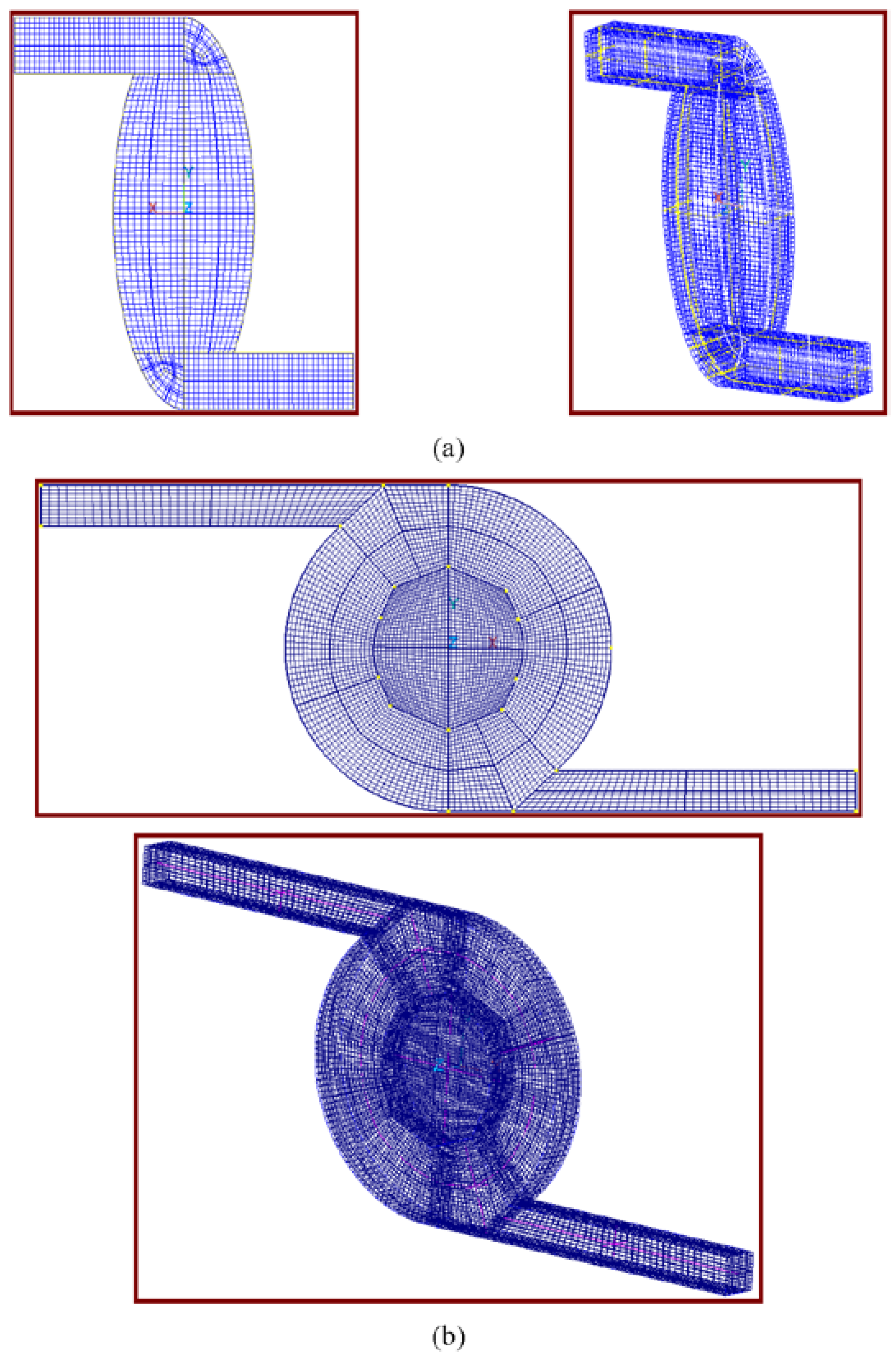
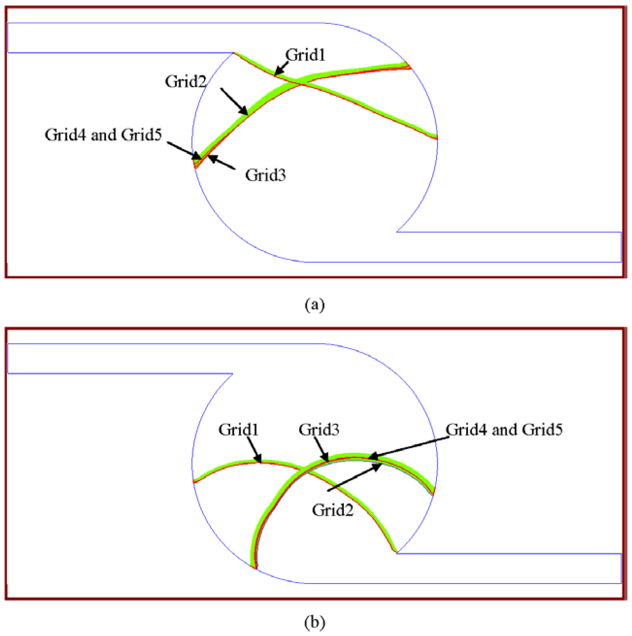
This work considers a configuration of the flow systems. It comprises inlet/outlet microchannels and a circular or an oval disk-shaped microchamber with an adhesive wall surface. The grid systems in the computational domain are selected to ensure the orthogonality, the smoothness and the low aspect ratios that prevent numerical divergence, shown in
Figure 2. Poor orthogonality most directly influences the accuracy of the flux calculations, whereas poor smoothness and high aspect ratios most directly affect the accuracy of the surface reconstruction. Grid size sensitivity was analyzed at the very beginning of the numerical simulations. Mesh density is increased continuously until it has minimal effects on the maximum velocity inside the system.
Figure 3 shows the shapes of the liquid fronts at times of 0.02 s and 0.04 s at an inlet flow velocity of 0.1 m/s. The analyses of five mesh densities ranging from 1.2096 × 10
4 to 1.6033 × 10
5 are used and the two finest meshes give a negligible relative difference in their corresponding values which indicates they are mesh-independent. The values of maximum velocity inside the microchannel at two different times for the five mesh densities are also expressed in
Table 1. Finally, the mesh density with 9.6768 × 10
4 has been chosen for further investigation since the maximum velocities inside the microchannel are almost the same and the numerical results are grid-independent.
Figure 2.
The grid systems of the computation domain for (a) oval and (b) circle disk-shaped chambers.
Figure 2.
The grid systems of the computation domain for (a) oval and (b) circle disk-shaped chambers.
Figure 3.
The shapes of the liquid fronts at times of (a) 0.02 s and (b) 0.04 s at an inlet flow velocity of 0.1 m/s at five mesh densities. Grid1: 1.2096 × 10⁴, Grid2: 3.0720 × 10⁴, Grid3: 5.6000 × 10⁴, Grid4: 9.6768 × 10⁴, and Grid5: 1.6033 × 10⁵.
Figure 3.
The shapes of the liquid fronts at times of (a) 0.02 s and (b) 0.04 s at an inlet flow velocity of 0.1 m/s at five mesh densities. Grid1: 1.2096 × 10⁴, Grid2: 3.0720 × 10⁴, Grid3: 5.6000 × 10⁴, Grid4: 9.6768 × 10⁴, and Grid5: 1.6033 × 10⁵.
Table 1.
The analysis of the grid size independence.
Table 1.
The analysis of the grid size independence.
| Number of nodes | Maximum velocity at 0.02 s | Relative difference in maximum velocity at 0.02 s (%) | Maximum velocity at 0.04 s | Relative difference in maximum velocity at 0.04 s (%) |
|---|
| Grid1: 1.2096 × 10⁴ | 0.305065 | - | 0.311528 | - |
| Grid2: 3.0720 × 10⁴ | 0.195608 | 55.97 | 0.195607 | 59.26 |
| Grid3: 5.6000 × 10⁴ | 0.200395 | 2.39 | 0.200394 | 2.39 |
| Grid4: 9.6768 × 10⁴ | 0.203124 | 1.34 | 0.203124 | 1.34 |
| Grid5: 1.6033 × 10⁵ | 0.204233 | 0.54 | 0.204233 | 0.54 |
4. Results and Discussion
In this section, two configurations of the flow network system are considered. The microchannels are 100 μm wide, 100 μm deep, and the circular disk-shaped microchamber has a diameter of 800 μm. These dimensions correspond to angles between the microchannel and the microchamber at the intersection of 138.6°. The microchannels are 100 μm wide in the oval disk-shaped microchamber for 700 μm and 250 μm of the semi-major and semi-minor axes. These dimensions correspond to angles between the microchannel and the microchamber at the intersection of 111.9°. The chambers may have hydrophilic or hydrophobic surfaces. The contact angle of the air-water interface on the solid surface is specified to simulate filling under various surface conditions and to elucidate the mechanism by which the front changes in the chamber. In the following, the effects of the various parameters on the motion and the shape of the air-water interface in a circular disk-shaped chamber are studied first. Then, the comparisons between numerical and experimental results are shown. The above values of the parameters are used unless otherwise stated.
In an effort to understand the surface tension flows inside microfluidic chips, the changes in the shape of the liquid front are used to evaluate the liquid filling processes.
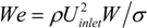
Figure 5 and
Figure 6 plot the effects of various inlet velocities on the filling process for a microstructure. Weber numbers of 0.345 and 0.0138, and Reynolds numbers of 50 and 10, are considered, corresponding to inlet flow velocities of 0.5 and 0.1 m/s, respectively. The Weber number is the ratio of the inertia to the surface tension, and is given by
![Micromachines 05 00116 i012]()
. The Reynolds number is the ratio of the inertia to the viscosity and is given by Re =
UinletW/
v where
Uinlet is the inlet flow velocity and W is the width of the microchannel.
ν and σ are the kinematic viscosity and the surface tension of the liquid, respectively. The static contact angle of the gas-liquid interface on a solid surface is used and taken to be 80°. In
Figure 5, the fluid enters an inlet channel at a pumping velocity of 0.1 m/s. It presents the locations of the air-water interface as a function of time for
t = 0.58 × 10
−2, 0.77 × 10
−2, 0.85 × 10
−2, 1.54 × 10
−2, 2.72 × 10
−2, 4.06 × 10
−2, 4.62 × 10
−2, 5.37 × 10
−2, 6.16 × 10
−2, 6.24 × 10
−2, and 6.43 × 10
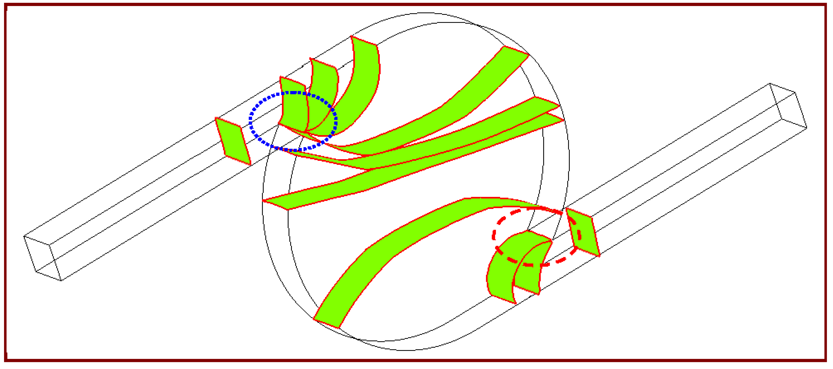
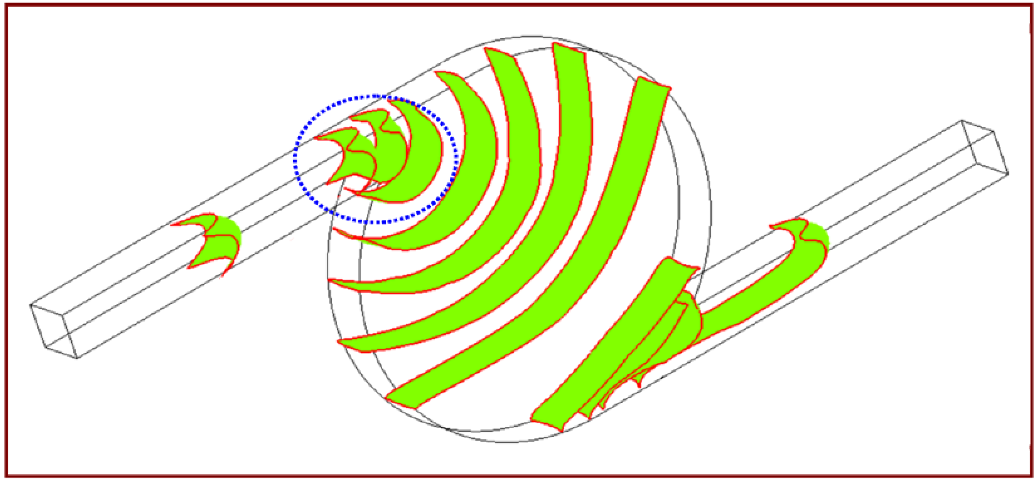
−2 s, respectively. The liquid flows forward and approaches the entrance of the chamber. Regarding the contact angle of 80°, the liquid has a concave interface with air. When the interface reaches the sharp corner, the meniscus near this corner stops moving forward and remains at this point until the bulk of the flow has advanced sufficiently, allowing the meniscus to bulge sufficiently over the corner so that the contact angle at the edge reaches 80° (marked by a blue dotted circle). The adhesive force between the liquid and the solid wall is established to create a capillary pressure barrier that stops the flow. An abrupt enlargement in the cross-sectional area for the contact angle of 80° makes the pressure in the liquid become negative. Then, the capillary gating effect can be seen. At this point, the angle of the liquid meniscus must change to adopt the equilibrium contact angle at the slanted walls. This side of the meniscus descends down the side of the chamber and along the surface. The other side of the meniscus keeps moving forward until it reaches the entrance of the chamber, because the wall of the inlet channel is tangential to the wall of the chamber and the inertia force continues to drive the liquid flow forward. Then, the flow leaves the inlet channel, wetting the side surface. This change in the angle between the microchannels and the microchamber at the intersection increases the gas-liquid area to more than the solid-liquid area for a given volume change, resulting in a negative opposing pressure. The surface tension of the meniscus and the liquid pumping force overcome this capillary pressure barrier that develops when the cross section of the channel changes abruptly, establishing a positive pressure that pulls the liquid into the microchamber. We is equal to 0.0138, so the surface tension dominates the flow mechanism. As the liquid flows into the chamber, the flow front becomes convex because of the inertia of the fluid flow. The curvature of the wall of the chamber changes the shape of the front such that it becomes flat when the liquid occupies almost one-third of the chamber volume. Then the shape becomes concave. The variations in the shape of the front are related directly to the inertia force and the properties of the wall. When the liquid meniscus reaches the outlet channel, one side of the liquid meniscus reaches the sharp corner, and it stops moving forward (marked by a red dashed circle). The other side of the meniscus continues to flow through the chamber. When the angle of the liquid meniscus changes to the equilibrium contact angle at the sharp corner, the gas-liquid interface exits through the outlet channel. The results indicate that the changed angles at the entrance and the exit of the chamber are closely related to the flow progression when geometric changes occur at the connections between the chamber and the channels. Finally, the liquid completes the filling process.
Figure 5.
Filling process for inlet velocity of 0.1 m/s and θs of 80°.
Figure 5.
Filling process for inlet velocity of 0.1 m/s and θs of 80°.
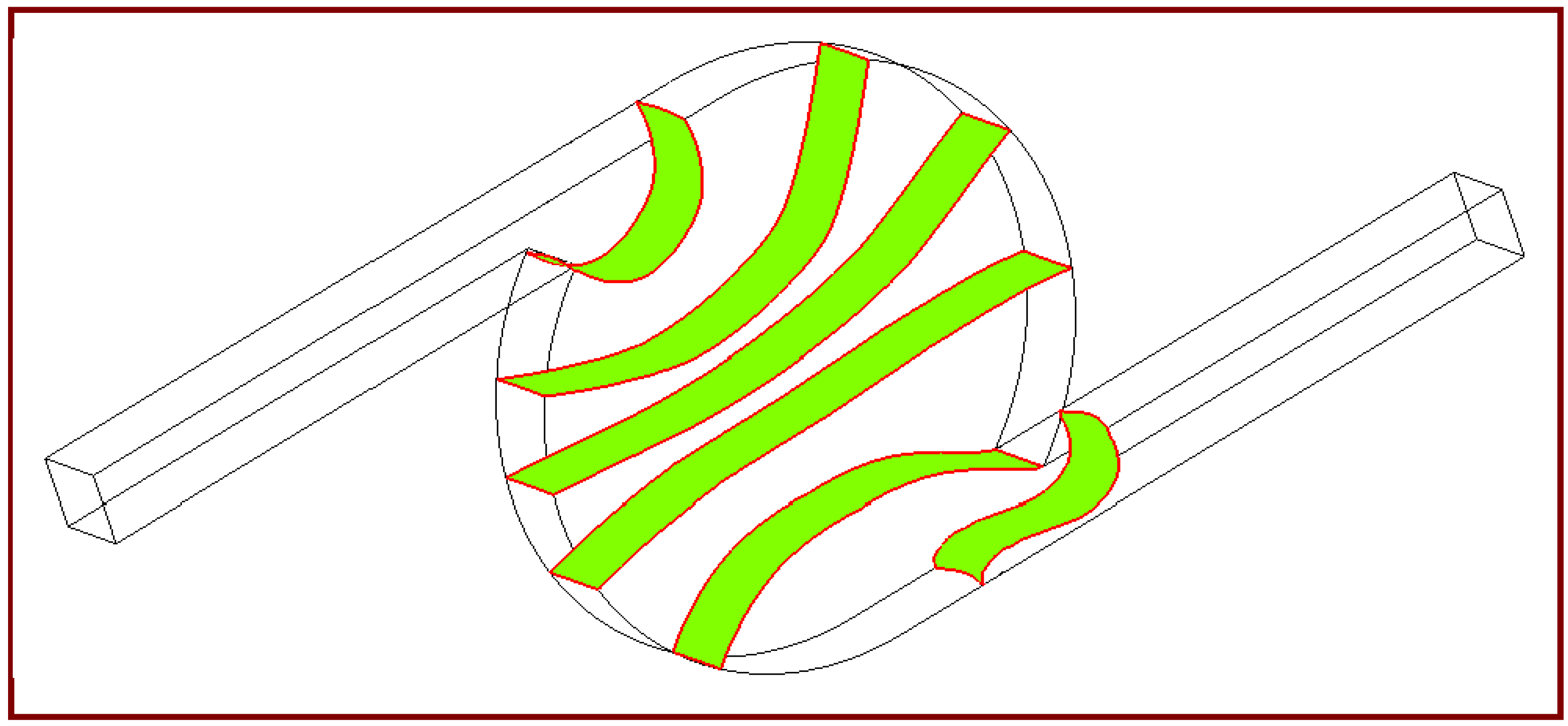
Re increases with the inlet velocity and the inertia force becomes dominant, as presented in
Figure 6. An 80° static contact angle of the gas-liquid interface on a solid surface is used. The figure presents the results for
t = 1.57 × 10
−3, 3.34 × 10
−3, 5.17 × 10
−3, 7.02 × 10
−3, 9.29 × 10
−3 and 12.47 × 10
−3 s, respectively, at an inlet velocity of 0.5 m/s. As the free surface reaches the sharp corner at the entrance of the chamber, the gas-liquid interface near this corner stops moving. The other side of the free surface keeps moving. The inertial force causes the meniscus to move faster; it overcomes the flow resistance at the corner easily and drives the fluid flowing into the chamber. The strong inertial force causes the interface to remain convex for almost two-thirds of the chamber volume. In
Figure 6, the wave front shape is changed from convex to flat and then to concave. When the fluid flows into the outlet channel, inertia force pushes the free surface concave at one side and convex at the other side. Finally, the filling process is finished without the entrapment of air bubbles. The competition between inertia and adhesion causes the shape to be linear inside the chamber for a long time.
Figure 6.
Filling process for inlet velocity of 0.5 m/s and θs of 80°.
Figure 6.
Filling process for inlet velocity of 0.5 m/s and θs of 80°.
When the liquid flows through the microstructure, a precise agreement between simulated data and experimental results is complicated [
27]. Simulations are mostly generated by applying a static contact angle at the boundary conditions. However, the contact angle depends on the velocity of the moving contact line. The velocity-dependent contact angles must be realized for the accurate calculation of surface tension forces.
Figure 7 shows the simulated velocity vectors as the liquid flows into the microstructure. We of 0.345 and Re of 50 are used, corresponding to an inlet flow velocity of 0.5 m/s. The surface tension force dominates this case. Three different models of the contact angle variation with contact line velocity,
vt, are employed on predictions of the liquid filling processes. The single ramp model, the stretched hyperbolic tangent model and the quadratic model are utilized to compare these simulations, shown from left to right in
Figure 7a–c, respectively. Among these models,
θs, static contact angle, is 80°,
θlc, lower cutoff angle, is 45°, and
θuc, upper cutoff angle, is 115°. In the single ramp model,
K, the slope of the function, is 350° s/m. In the stretched hyperbolic tangent model,
a is 10° s
2/m
2,
b is 0° s/m, and
c is 0°. In the quadratic model,
a is 1750 s
3/m
3,
b is 350 s
2/m
2, and
c is 62.5 s/m. The functional dependences are shown in
Figure 1. When the liquid-gas interface does not move,
i.e.,
vt equals 0 m/s, the static contact angle is used. The contact angle is considered increased with the increasing of
vt. From the top to the bottom in
Figure 7, the results are present the results for
t = 1.33 × 10
−3, 2.61 × 10
−3, 10.51 × 10
−3, and 12.57 × 10
−3 s, respectively. The difference is almost negligible at the four times. It means that the liquid filling processes inside our microstructures are approximately the same among three functional forms with specific parameters. The overall computational time for predicting the filling processes in our system by using the single ramp model, the stretched hyperbolic tangent model and the quadratic model is about 36 h, 51 h, and 53 h per case, respectively, using a computer with Intel
® Core™2 Duo CPU T8300 and 2G RAM. However, the computational time for predicting the liquid filling process in our system is the shortest by using the single ramp model. Thus the single ramp model is chosen to prevent a lot of additional computational time in the following simulations.
Figure 7.
Filling process for three models: (a) single ramp model; (b) stretched hyperbolic tangent model; and (c) quadratic model.
Figure 7.
Filling process for three models: (a) single ramp model; (b) stretched hyperbolic tangent model; and (c) quadratic model.
Figure 8 plots the results concerning the motion of the gas-liquid interface at a velocity-dependent contact angle of a single ramp model presented in
Figure 7. In this case,
K is equal to 350° s/m,
θs is 80°,
θlc is 45°, and
θuc is 115°. It means that the contact angle increases linearly with
vt from 80° to 115° while
vt is under 0.1 m/s, and the contact angle is invariant and equal to 115° while
vt is greater than 0.1 m/s. When the gas-liquid interface reaches the sharp corner near the inlet or the outlet channel, the meniscus near this corner moves slowly and remains at the corners until the bulk of the flow has sufficiently advanced. Concerning the wall adhesion properties, the wall is under a hydrophilic condition (
θd is less than 90°) as
vt is less than 0.03 m/s. The effect of a capillary pressure barrier does not remain obvious; the flow front keeps moving into the chamber without stopping (marked by a blue dotted circle). Compared with the results marked by a blue dotted circle in
Figure 5, the adhesive force between the liquid and the solid wall is established to create a capillary pressure barrier that stops the flow by regarding the static contact angle condition. Considering the dynamic contact angle model in
Figure 8, the capillary pressure barrier near the sharp corner is negligible. From our previous results [
27], the flow front shapes differ between numerical and experimental date in which the flow front enters the chamber after it passed around the sharp corner. It is found that the flow front progresses into the chamber without stopping from visualized images. By utilizing the dynamic contact angle model, the simulations compared with our experimental results [
27] show a similar trend. When the liquid moves into the chamber and the cross-sectional area becomes large, the velocity of the gas-liquid interface starts to decrease. With regard to the wall adhesion properties, the wall is under a hydrophilic condition. The liquid moves along the circular chamber wall, and the flow is still driven by the inertia, so the meniscus bulges while entering the microchamber. Given a hydrophilic wall, the front is convex and then concave as the liquid flows through the chamber while wetting the side surface.
Figure 8.
Filling process for the single ramp model when K is 350° s/m, θs is 80°, θlc is 45° and θuc is 115°.
Figure 8.
Filling process for the single ramp model when K is 350° s/m, θs is 80°, θlc is 45° and θuc is 115°.
The effect of the parameters of the single ramp function at an inlet flow velocity of 0.25 m/s is studied and demonstrated in
Figure 9. We equals 0.0863, and Re equals 25. When the liquid flows into the microstructure, the liquid/surface contact angle ranges between 50° and 85°, 80° and 115°, 110° and 145° for cases (a), (b), and (c), respectively. From the top to the bottom in
Figure 9, the results are present the results for
t = 0.09 × 10
−2, 0.30 × 10
−2, 0.73 × 10
−2, 0.94 × 10
−2, 1.19 × 10
−2, and 1.33 × 10
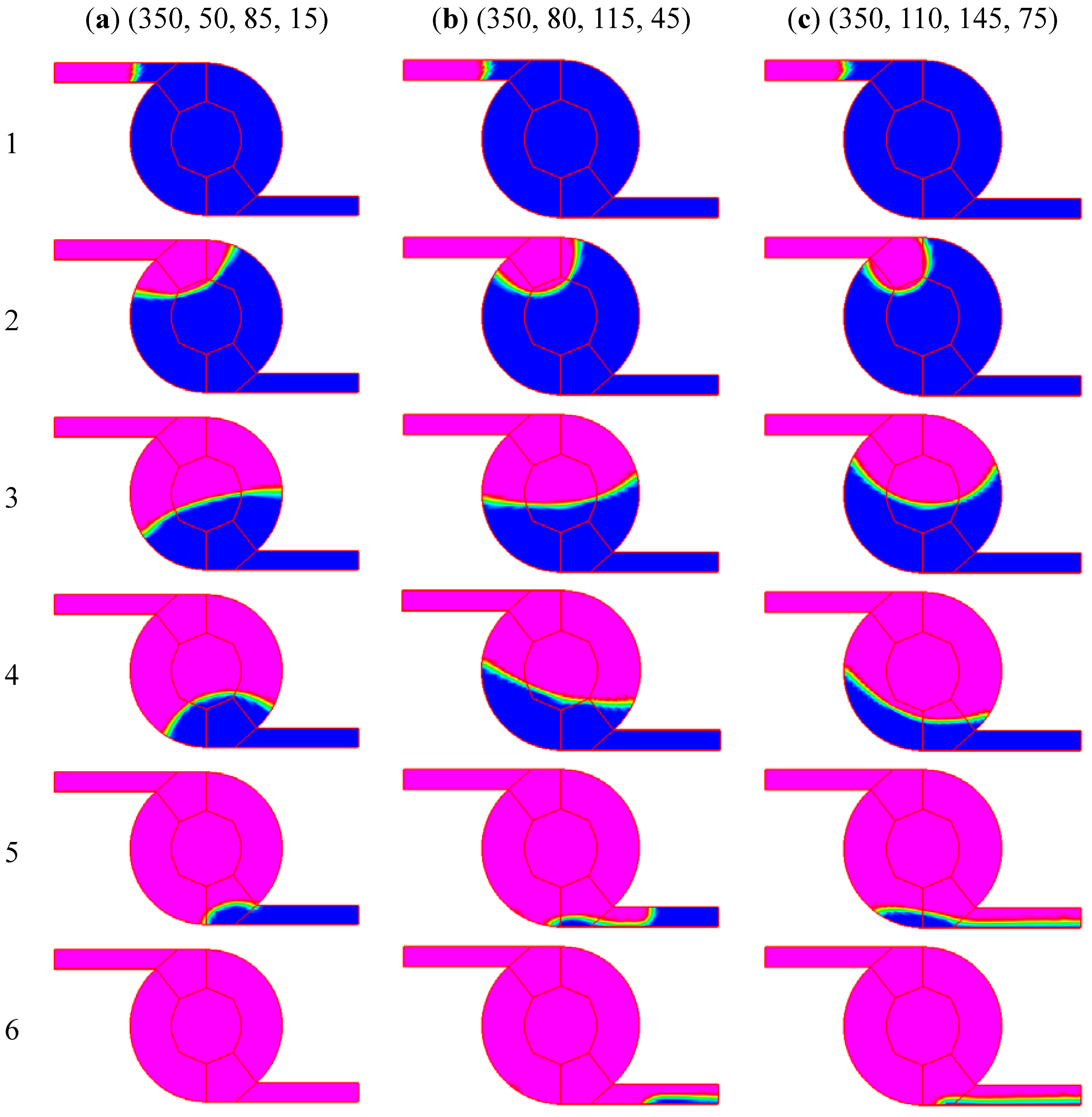
−2 s, respectively. For a hydrophilic wall in case (a), the flow front keeps moving into the chamber without stopping because of surface tension and inertia. When the surface tension dominates, the fluid flows into the chamber, wetting the side surface, and the effect of a capillary pressure barrier does not remain obvious. When the liquid moves into the chamber, the increase in the cross-sectional area of the chamber reduces the inertia. The interface stops moving at the sharp corner near the exit of the chamber and its angle changes to the contact angle. The interface retains its concave shape throughout the filling process. Given a hydrophobic wall for case (c), the front is convex as the liquid flows through the chamber without wetting the side surface. After the meniscus reaches the sharp corner near the inlet or the outlet channel, it remains at the corners until the bulk of the flow has sufficiently advanced. The liquid flow is still driven by the inertia, so the meniscus bulges over the whole chamber. The wave front becomes attached to the wall before the meniscus stretches across the whole chamber. The meniscus bulges sufficiently over the sharp corner near the outlet channel so the contact angle at the edge reaches imposed conditions.
Figure 9.
Filling process for various θs, θlc and θuc. (a) K is 350° s/m, θs is 50°, θlc is 15° and θuc is 85°; (b) K is 350° s/m, θs is 80°, θlc is 45° and θuc is 115°; and (c) K is 350° s/m, θs is 110°, θlc is 75° and θuc is 145°.
Figure 9.
Filling process for various θs, θlc and θuc. (a) K is 350° s/m, θs is 50°, θlc is 15° and θuc is 85°; (b) K is 350° s/m, θs is 80°, θlc is 45° and θuc is 115°; and (c) K is 350° s/m, θs is 110°, θlc is 75° and θuc is 145°.
From the previous work [
18], it is presented that the contact angle increases with the increasing of the contact line velocity. For the single ramp function,
K denotes the slope of the function. When
K is large, the contact angle increases much as the contact line velocity becomes large.
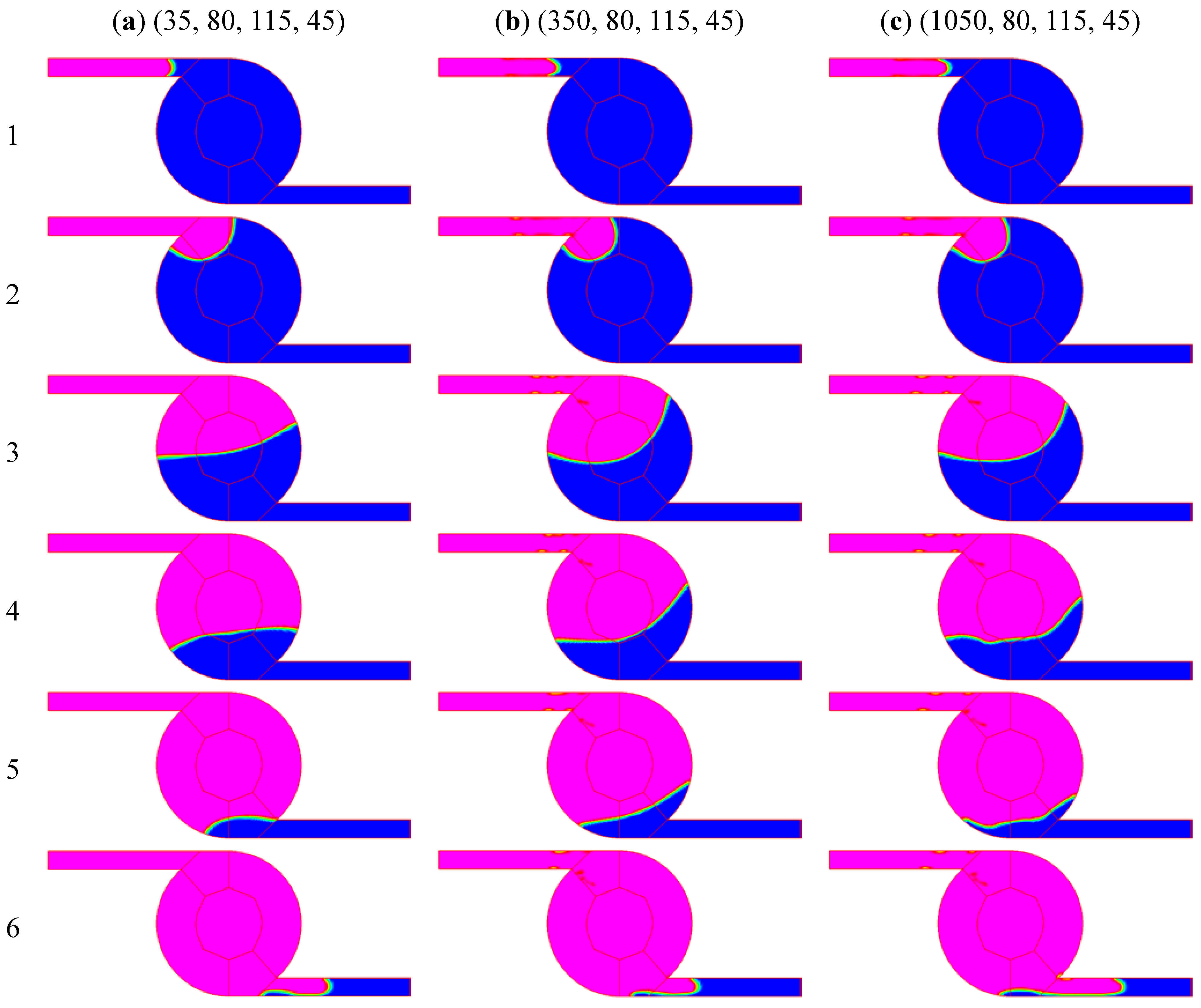
Figure 10 illustrates the results concerning the motion of the gas-liquid interface at various slopes of the single ramp function. In this case,
θs is 80°,
θlc is 45°, and
θuc is 115°.
K, the slope, is equal to 35° s/m, 350° s/m, and 1050° s/m, respectively, from left to right in
Figure 10(a) to 10(c). It means that the contact angle increases linearly with the contact line velocity from 80° to 115° while
vt is under 1, 0.1, and 0.033 m/s, and the contact angle is equal to 115° while
vt is greater than 1, 0.1, and 0.033 m/s, respectively. From the top to the bottom in
Figure 10, the results are present the results for
t = 0.08 × 10
−2, 0.30 × 10
−2, 0.73 × 10
−2, 0.98 × 10
−2, 1.19 × 10
−2, and 1.34 × 10
−2 s, respectively. When
K is 35° s/m, the microstructure for the liquid flow is generally under a hydrophilic wall condition (the contact angle is less than 90°) as
vt is less than 0.286 m/s. The flow front keeps moving into the chamber without stopping. The effect of a capillary pressure barrier does not remain obvious. The interface stops moving at the sharp corner near the exit of the chamber and its angle changes to the contact angle. The same feature profile is used in
Figure 10, but
K is increased to 1050° s/m. A hydrophobic wall is generated (the contact angle is larger than 90°) when
vt is greater than 0.001 m/s. The front is convex as the liquid flows through the chamber without wetting the side surface. After the meniscus reaches the sharp corner near the inlet or the outlet channel,
vt starts to decrease. Then the contact angle decreases and the walls become hydrophilic. The flow front keeps moving into the chamber or the outlet channel without stopping. The liquid flow is still driven by the inertia, so the meniscus bulges over the whole chamber. The interface descends along the outlet channel so air is almost entrapped.
Finally, experimental and numerical studies of surface tension-driven flow in our surface-modified microstructures are performed. Because of the hydrophobicity of the PDMS, an oxygen plasma treatment is used to modify the surface of the PDMS substrate. Then the surface of PDMS microstructures can be modified to be hydrophilic. Thus flow experiments are conducted into both hydrophilic and hydrophobic PDMS microstructures. In
Figure 11, PDMS is used as a cover under which the PDMS microstructure is fabricated using MEMS technology. The oxidized PDMS surface slowly recovers its hydrophobicity after exposure to the ambient after one day. This PDMS is almost completely transparent in the visible spectrum. Flow experiments are conducted at least four times, under the same conditions, to confirm repeatability. In each experiment, the total filling time is measured with a deviation of the order of 0.001 s. The experimental observations described below were repeatable.
Figure 11 presents many experimental results obtained in an oval microchamber and the microchannels are 100 μm wide and 100 μm deep with an inlet velocity of 0.02 m/s. One set of lengths of the semi-major and semi-minor axes of the oval disk-shaped chamber are 700 μm/250 μm. From the top to the bottom in
Figure 11, the results are present the results for
t = 3.42 × 10
−1, 4.78 × 10
−1, 6.24 × 10
−1, and 8.52 × 10
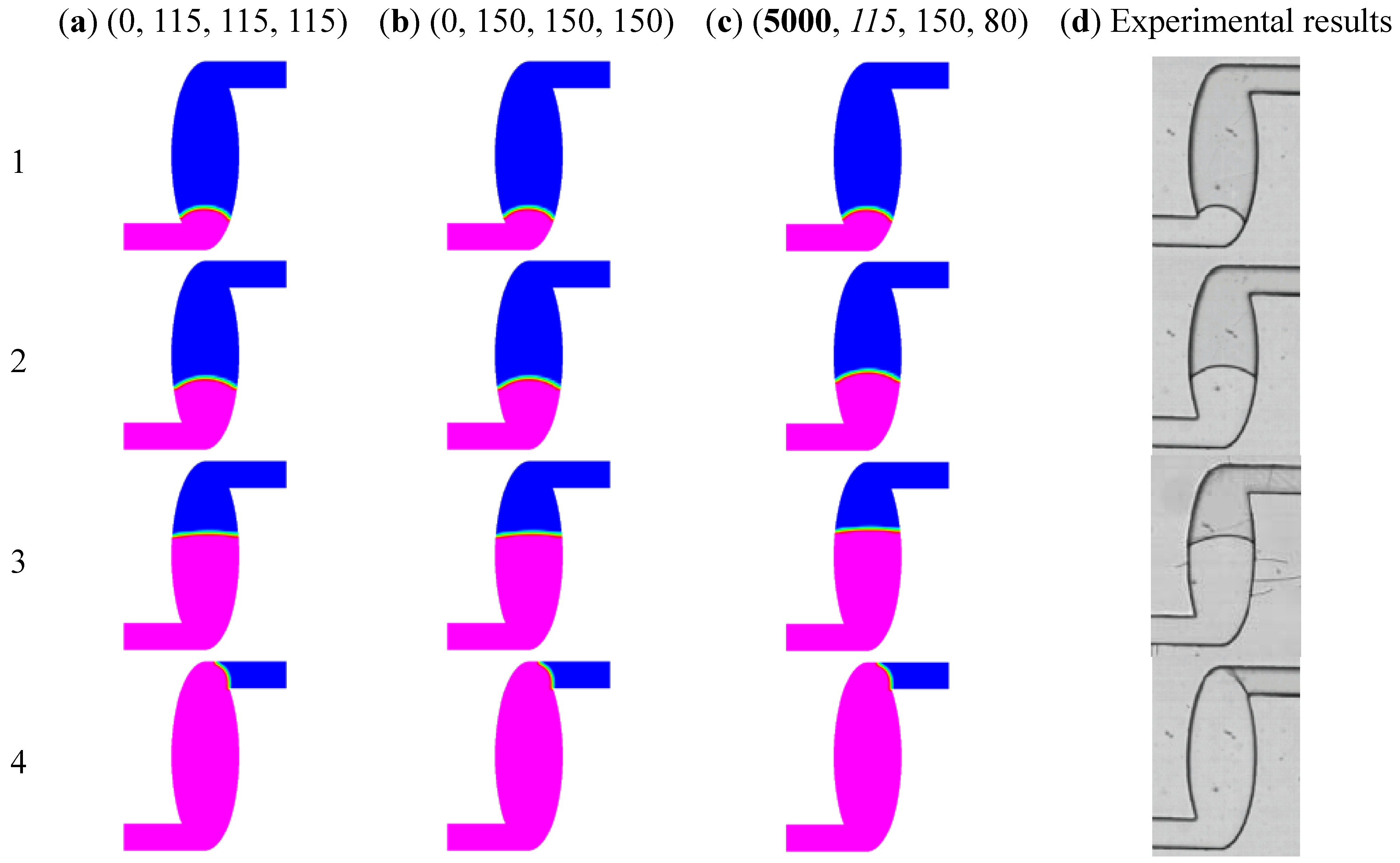
−1 s, respectively. The results are confirmed by numerical simulation and experimental interface locations. The numerical results are also compared with experimental measurements and reveal similar filling processes. The parameters of the functional form of the dynamic contact angle for each case are (
K,
θs,
θuc,
θlc). A static contact angle is specific at the walls as
K is equal to 0° s/m. The flow front shapes show similar results among case (a), (b), (c) and (d) experimental interface locations. The static contact angle of water on PDMS surface is about 105°. For a pressure-driven flow, a flow hindrance effect with regard to the surface tension can be seen, so the range of the contact angle varies from 90° to 180° [
2]. It means that the dynamic contact angles are still above 90° for a given hydrophobic condition. Results show that numerical simulations with imposed boundary conditions of static and dynamic contact angles can successfully predict the moving of the meniscus compared with experimental measurements.
A glass slide is also used to bond the PDMS replica. After O
2 plasma treatment and bonding, the designed microstructure has been fabricated. This chip is also almost completely transparent in the visible spectrum.
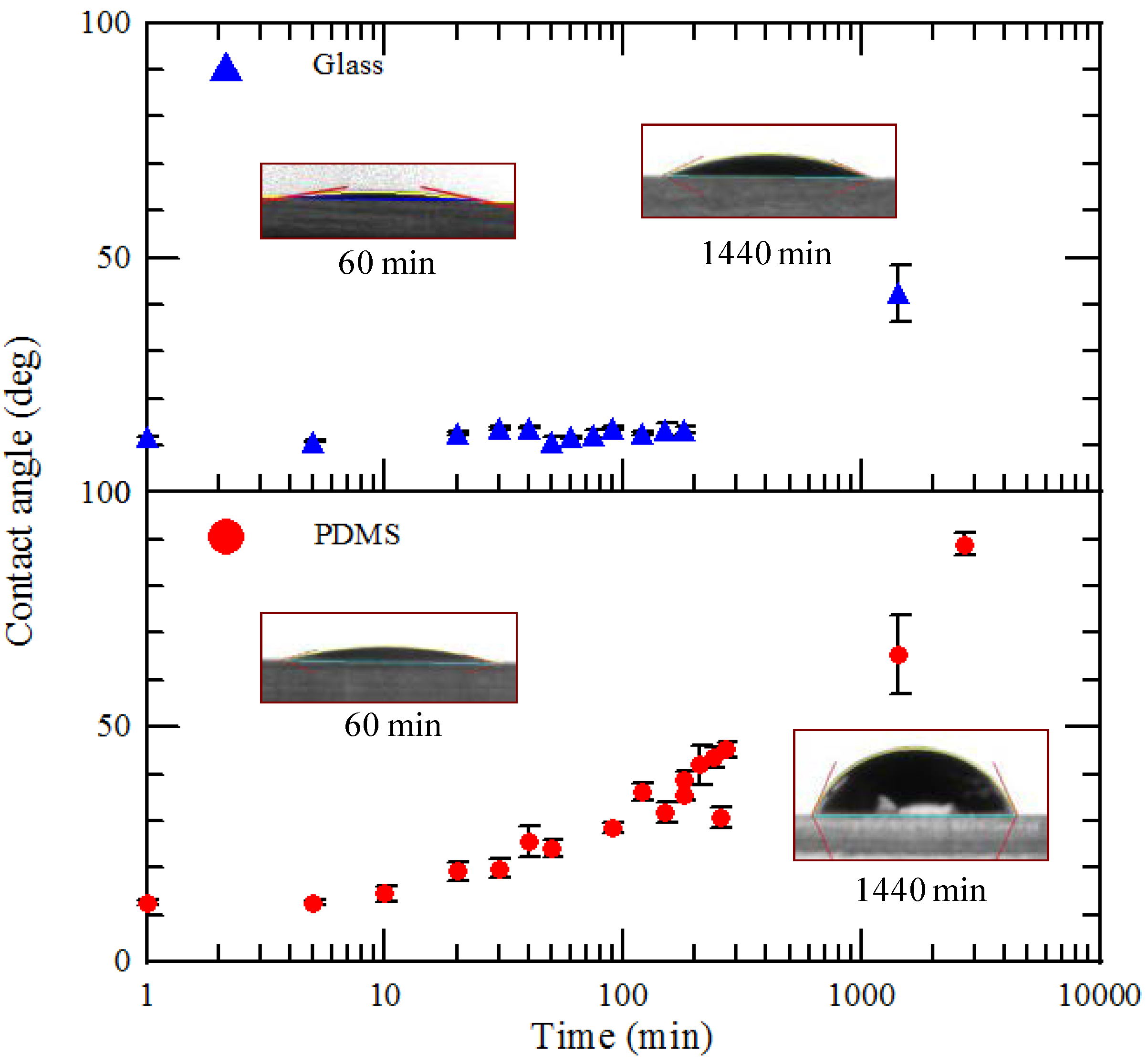
Figure 12 presents many experimental results obtained in similar conditions as those shown in
Figure 11. The experiments are conducted around one hour after the PDMS surface modification. The static contact angle of water on the surface of glass-PDMS bonding microstructure is about 30°, shown in
Figure 4. From the top to the bottom in
Figure 12, the results are present the results for
t = 2.33 × 10
−1, 3.62 × 10
−1, 4.29 × 10
−1, 5.63 × 10
−1, and 6.91 × 10
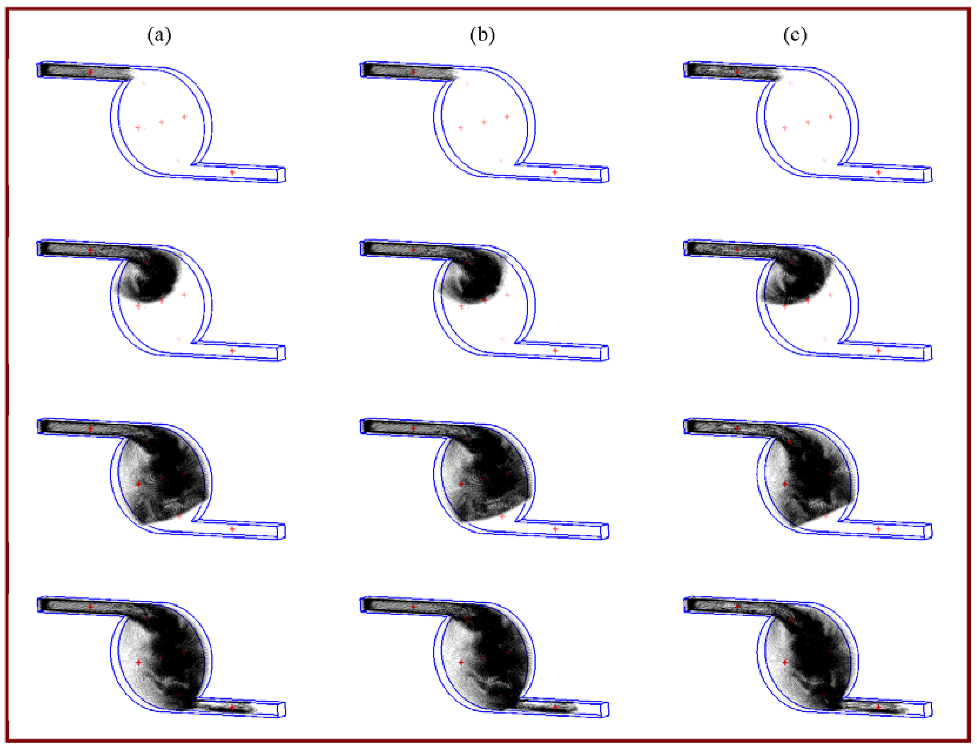
−1 s, respectively. And it can be seen that the static contact angle remains the similar value at 40 min to 100 min after the oxygen treatment process. A flow hindrance effect with regard to the surface tension for a pressure-driven flow can cause the contact angle to range from 90° to 180°. The assumed hydrophilic and hydrophobic wall conditions for cases (a) and (b), respectively, cannot be used for accurate calculation of surface tension forces. The flow front shapes show similar results only between case (c) and (d) experimental interface locations. Results show that numerical simulations with a single ramp functional model can successfully predict the moving of the meniscus compared with experimental measurements.
Figure 10.
Filling process for various K. (a) K is 35° s/m, θs is 80°, θlc is 45° and θuc is 115°; (b) K is 350° s/m, θs is 80°, θlc is 45° and θuc is 115°; and (c) K is 1050° s/m, θs is 80°, θlc is 45° and θuc is 115°.
Figure 10.
Filling process for various K. (a) K is 35° s/m, θs is 80°, θlc is 45° and θuc is 115°; (b) K is 350° s/m, θs is 80°, θlc is 45° and θuc is 115°; and (c) K is 1050° s/m, θs is 80°, θlc is 45° and θuc is 115°.
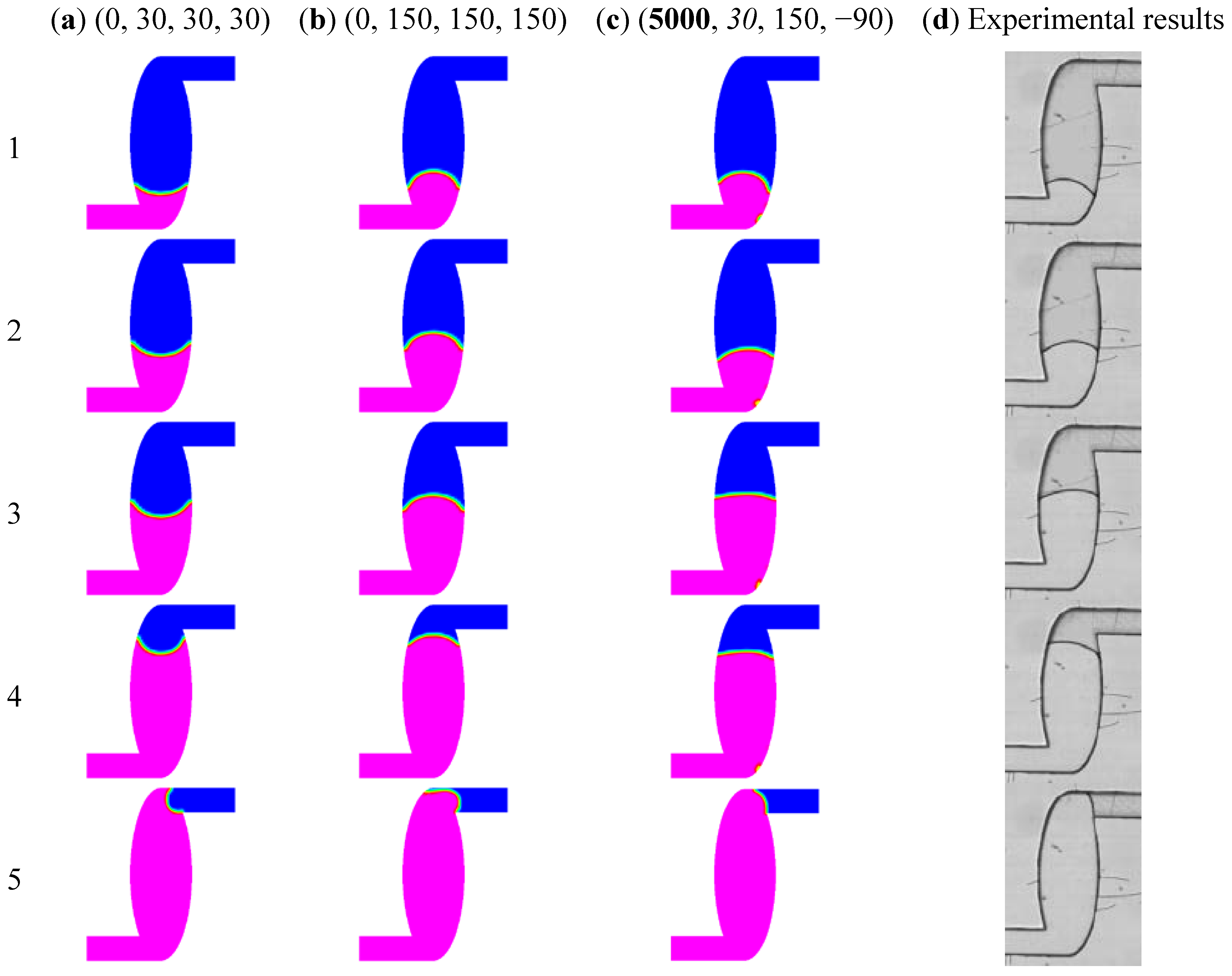
Figure 11.
Computational results corresponding to experimental measurements. (a) K is 0° s/m, θs is 115°, θlc is 115° and θuc is 115°; (b) K is 0° s/m, θs is 150°, θlc is 150° and θuc is 150°; and (c) K is 5000° s/m, θs is 115°, θlc is 80° and θuc is 150°; (d) photographs of a microchannel device showing liquid filling process.
Figure 12.
Computational results corresponding to experimental measurements. (a) K is 0° s/m, θs is 30°, θlc is 30° and θuc is 30°; (b) K is 0° s/m, θs is 150°, θlc is 150° and θuc is 150°; (c) K is 5000° s/m, θs is 30°, θlc is −90° and θuc is 150°; (d) photographs of a microchannel device showing liquid filling process.

 ,
, 
 is the fluid velocity vector.


 in the framework of the continuum surface force (CSF) model, which is ideally suited for the Eulerian interface of arbitrary topology [32,33]. In the Eulerian interface method the grid mesh in the numerical computation is fixed and the fluid and other objects flow across computational cells. The CSF model eliminates the need for detailed interface information and is commonly utilized in recent studies. We can express

 and
and  represent outward normal and tangential vectors for the walls, respectively. Therefore, F takes a unit value in cells that contain only liquid fluid, and zero in cells that contain only gas. A cell that contains an interface would have an F of between zero and unity.


 . The Reynolds number is the ratio of the inertia to the viscosity and is given by Re = UinletW/v where Uinlet is the inlet flow velocity and W is the width of the microchannel. ν and σ are the kinematic viscosity and the surface tension of the liquid, respectively. The static contact angle of the gas-liquid interface on a solid surface is used and taken to be 80°. In Figure 5, the fluid enters an inlet channel at a pumping velocity of 0.1 m/s. It presents the locations of the air-water interface as a function of time for t = 0.58 × 10⁻², 0.77 × 10⁻², 0.85 × 10⁻², 1.54 × 10⁻², 2.72 × 10⁻², 4.06 × 10⁻², 4.62 × 10⁻², 5.37 × 10⁻², 6.16 × 10⁻², 6.24 × 10⁻², and 6.43 × 10⁻² s, respectively. The liquid flows forward and approaches the entrance of the chamber. Regarding the contact angle of 80°, the liquid has a concave interface with air. When the interface reaches the sharp corner, the meniscus near this corner stops moving forward and remains at this point until the bulk of the flow has advanced sufficiently, allowing the meniscus to bulge sufficiently over the corner so that the contact angle at the edge reaches 80° (marked by a blue dotted circle). The adhesive force between the liquid and the solid wall is established to create a capillary pressure barrier that stops the flow. An abrupt enlargement in the cross-sectional area for the contact angle of 80° makes the pressure in the liquid become negative. Then, the capillary gating effect can be seen. At this point, the angle of the liquid meniscus must change to adopt the equilibrium contact angle at the slanted walls. This side of the meniscus descends down the side of the chamber and along the surface. The other side of the meniscus keeps moving forward until it reaches the entrance of the chamber, because the wall of the inlet channel is tangential to the wall of the chamber and the inertia force continues to drive the liquid flow forward. Then, the flow leaves the inlet channel, wetting the side surface. This change in the angle between the microchannels and the microchamber at the intersection increases the gas-liquid area to more than the solid-liquid area for a given volume change, resulting in a negative opposing pressure. The surface tension of the meniscus and the liquid pumping force overcome this capillary pressure barrier that develops when the cross section of the channel changes abruptly, establishing a positive pressure that pulls the liquid into the microchamber. We is equal to 0.0138, so the surface tension dominates the flow mechanism. As the liquid flows into the chamber, the flow front becomes convex because of the inertia of the fluid flow. The curvature of the wall of the chamber changes the shape of the front such that it becomes flat when the liquid occupies almost one-third of the chamber volume. Then the shape becomes concave. The variations in the shape of the front are related directly to the inertia force and the properties of the wall. When the liquid meniscus reaches the outlet channel, one side of the liquid meniscus reaches the sharp corner, and it stops moving forward (marked by a red dashed circle). The other side of the meniscus continues to flow through the chamber. When the angle of the liquid meniscus changes to the equilibrium contact angle at the sharp corner, the gas-liquid interface exits through the outlet channel. The results indicate that the changed angles at the entrance and the exit of the chamber are closely related to the flow progression when geometric changes occur at the connections between the chamber and the channels. Finally, the liquid completes the filling process.