
A Novel High-Precision Workpiece Self-Positioning Method for Improving the Convergence Ratio of Optical Components in Magnetorheological Finishing


Abstract
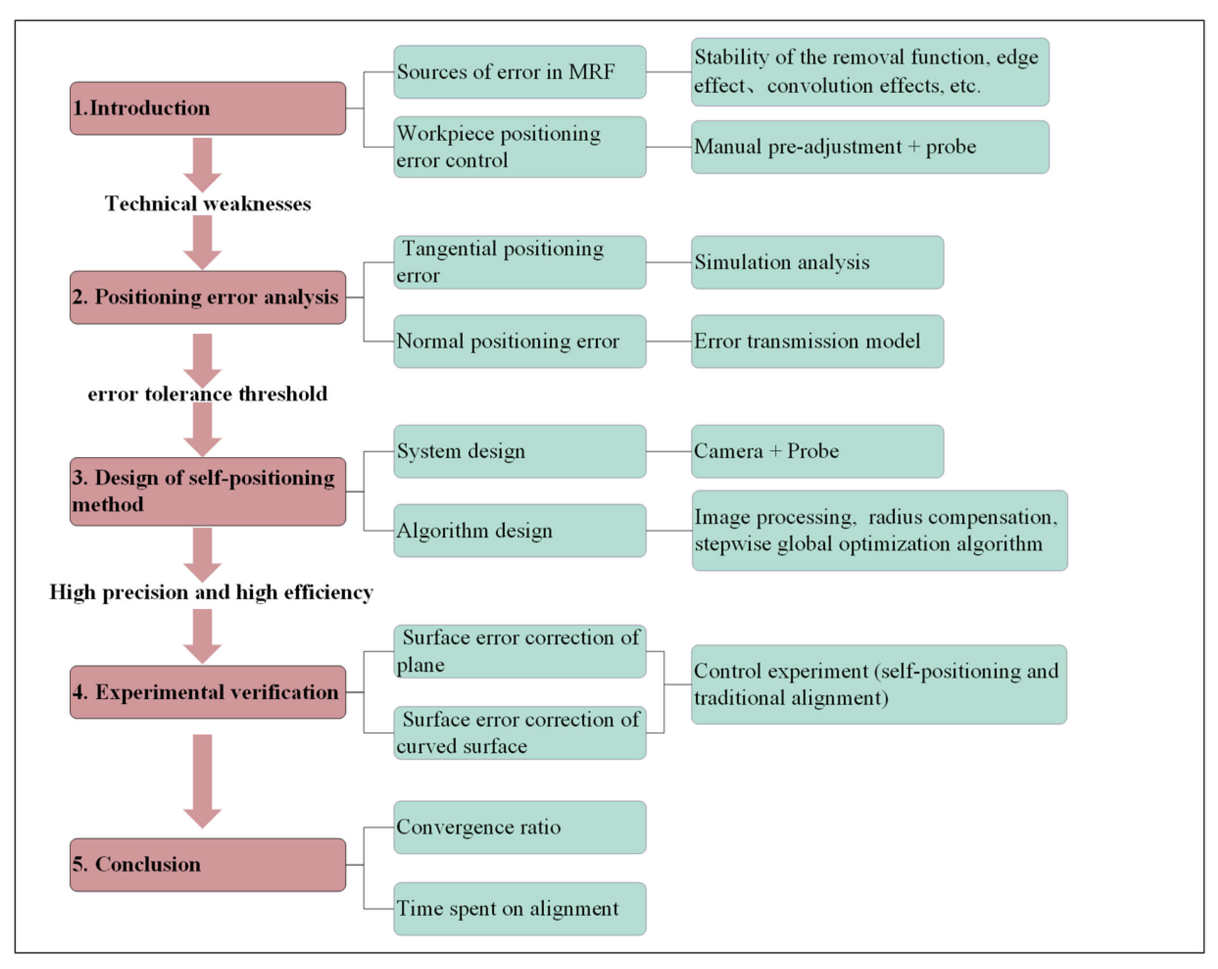
1. Introduction
2. Influence of Workpiece Positioning Errors on Polishing Convergence Ratio
2.1. Sources of Positioning Errors
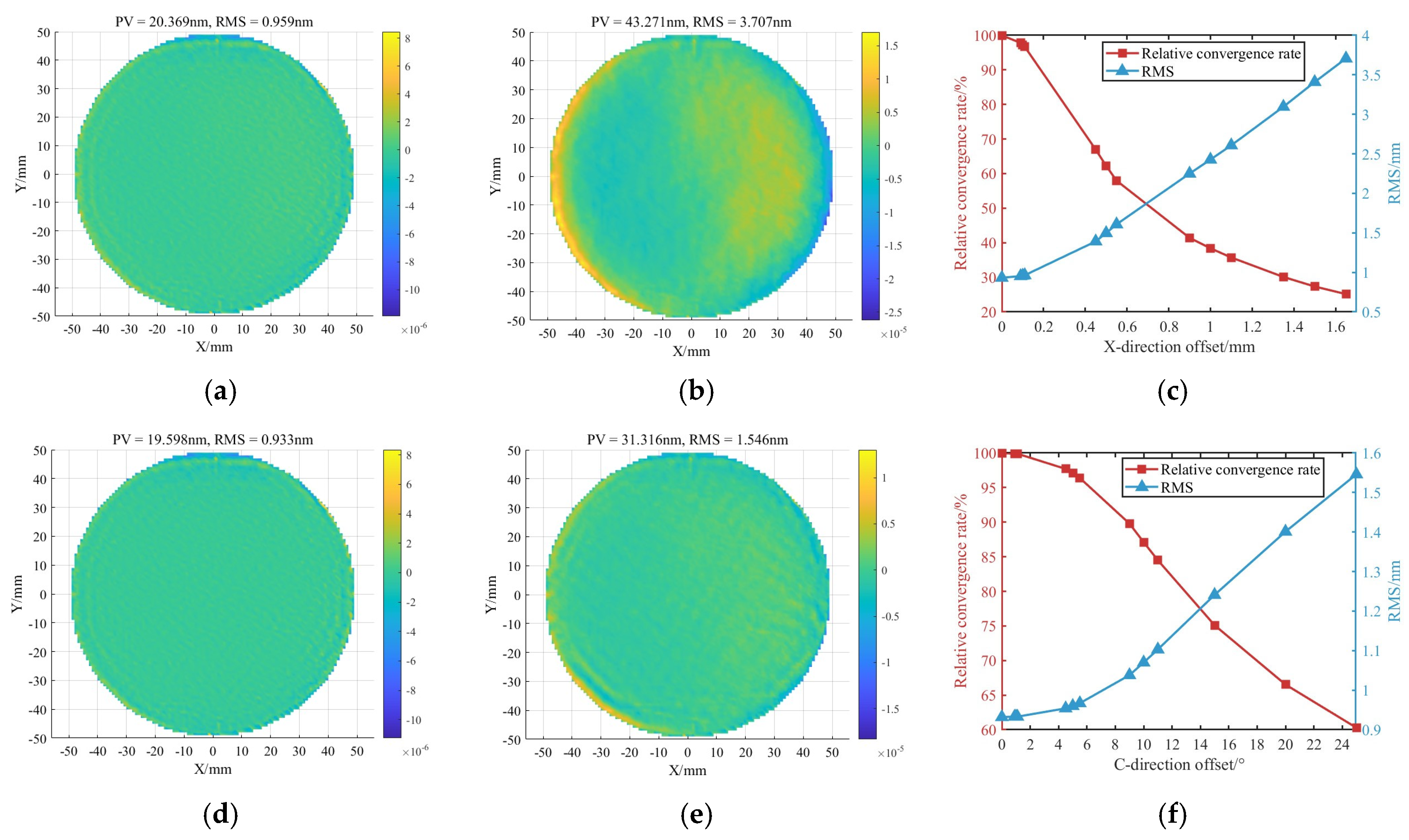
2.2. Tangential Positioning Error
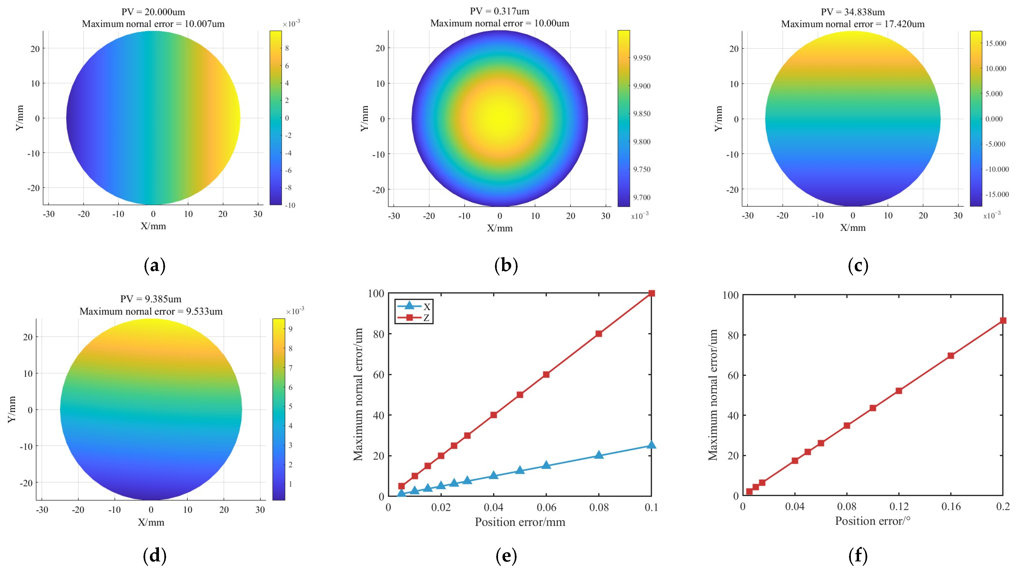
2.3. Normal Positioning Error
3. High-Precision Self-Positioning Method Design
3.1. Overall Design of the Self-Positioning Method
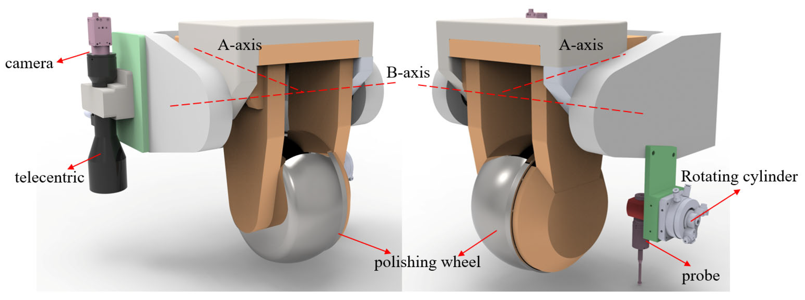
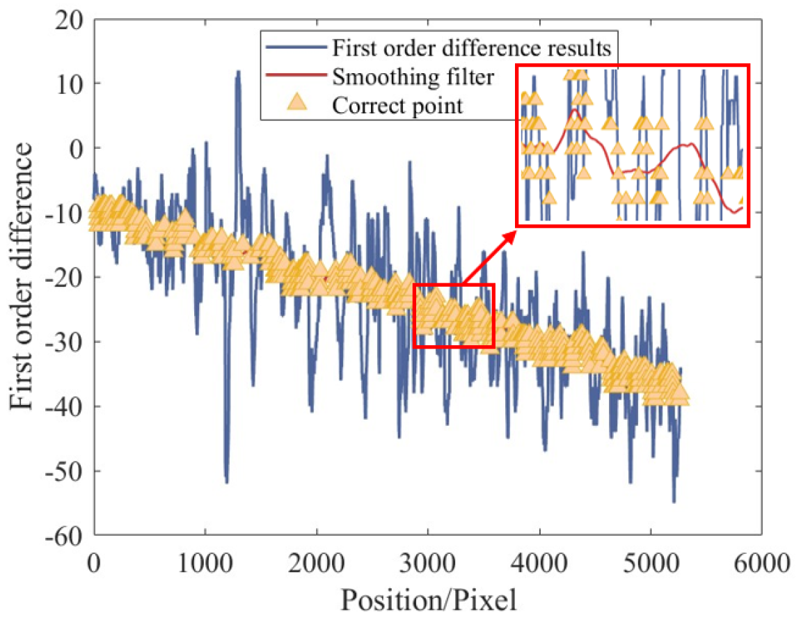
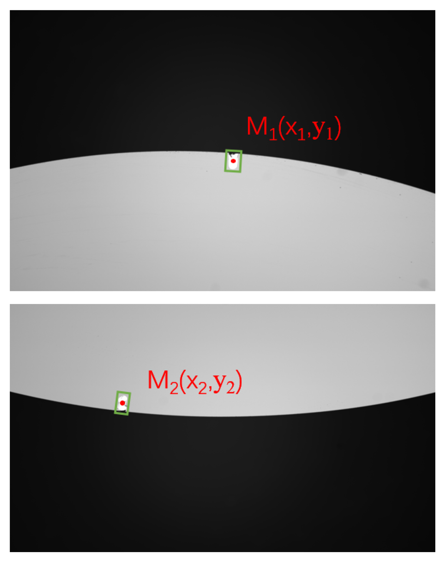
3.2. Vision-Based Center Localization Method
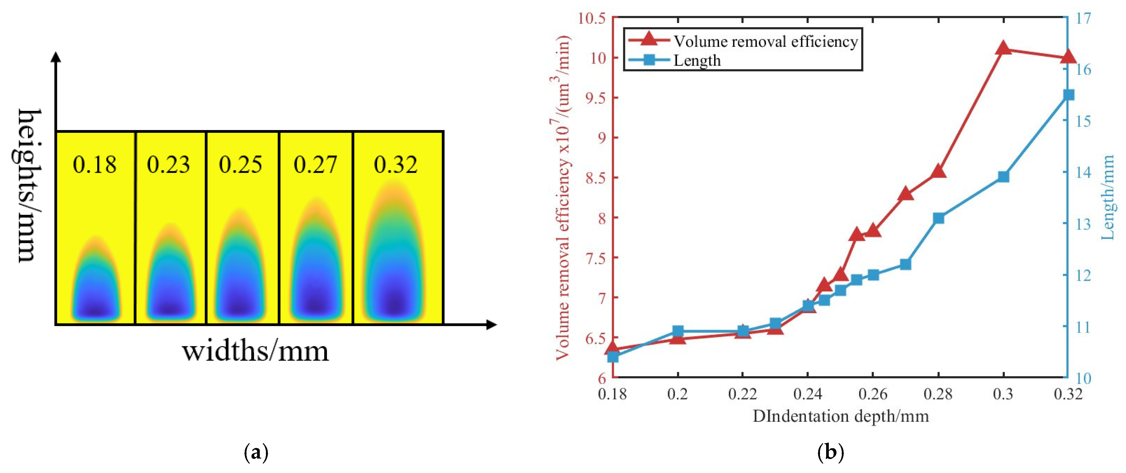
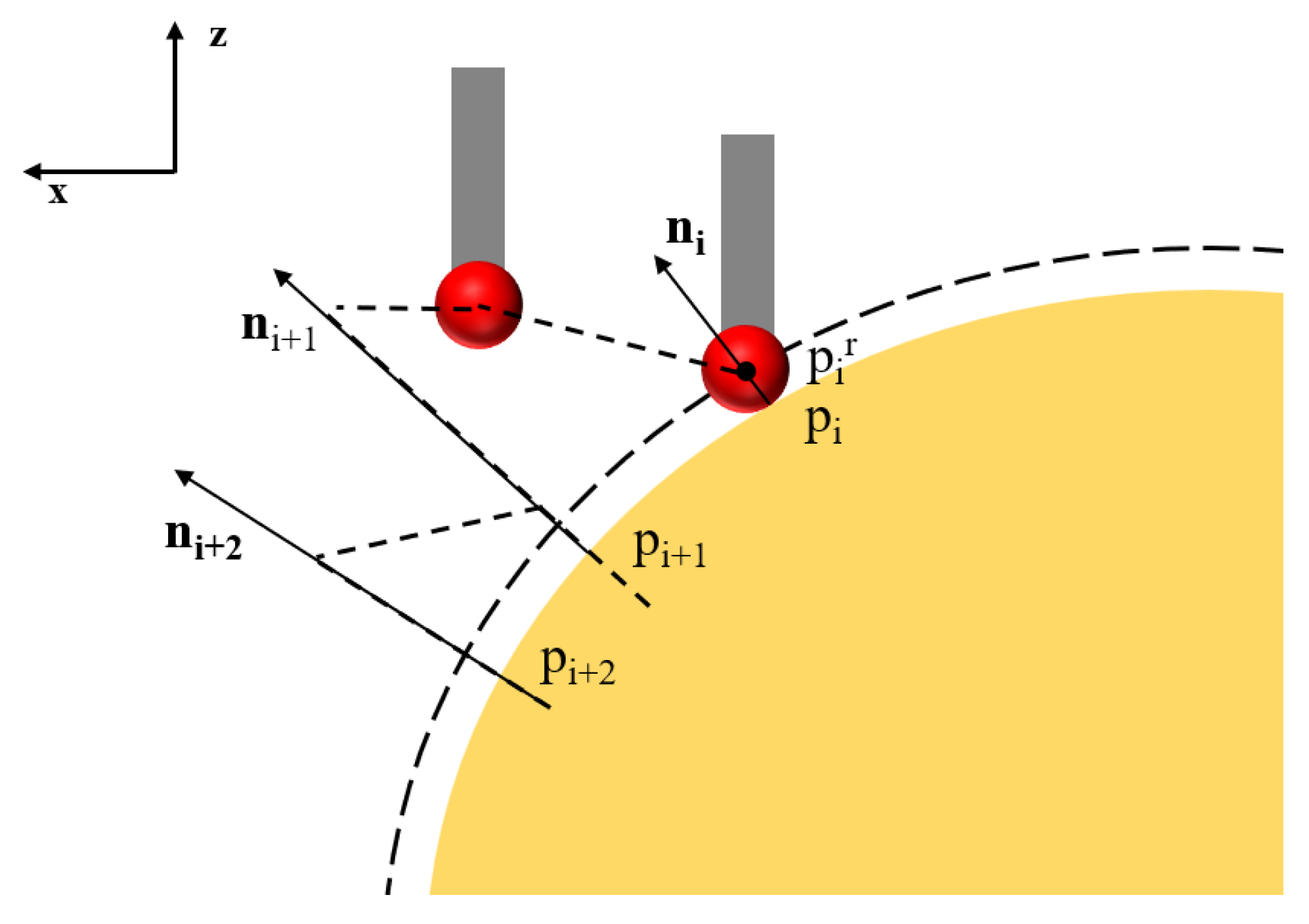
3.3. Probe Data Acquisition and Ball Tip Radius Compensation
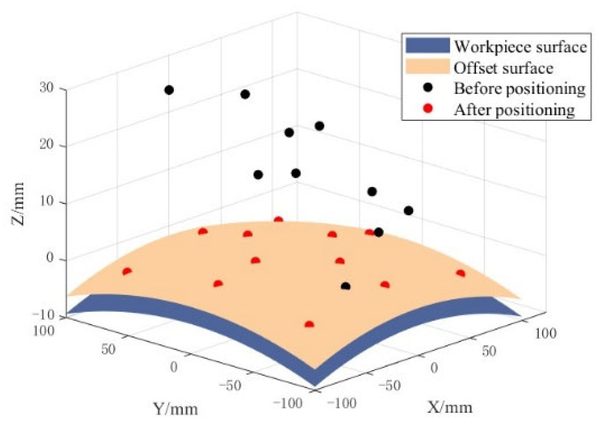
3.4. Design of a Stepwise Global Optimization Algorithm
4. Experimental Validation and Results Analysis
4.1. Experimental Platform and Test Conditions
4.2. Experimental Results
5. Discussion and Conclusions
- (1)
- A positioning error-normal contour error transmission model was established. Numerical simulations were conducted to analyze the impact of each degree of freedom on surface figure convergence. The results indicate that normal positioning errors have a far greater influence than tangential errors. Error tolerance thresholds were clearly defined: X/Y-direction errors ≤ 10 μm, Z-direction errors ≤ 5 μm, A/B-direction errors ≤ 0.005°, and C-direction errors ≤ 0.01°.
- (2)
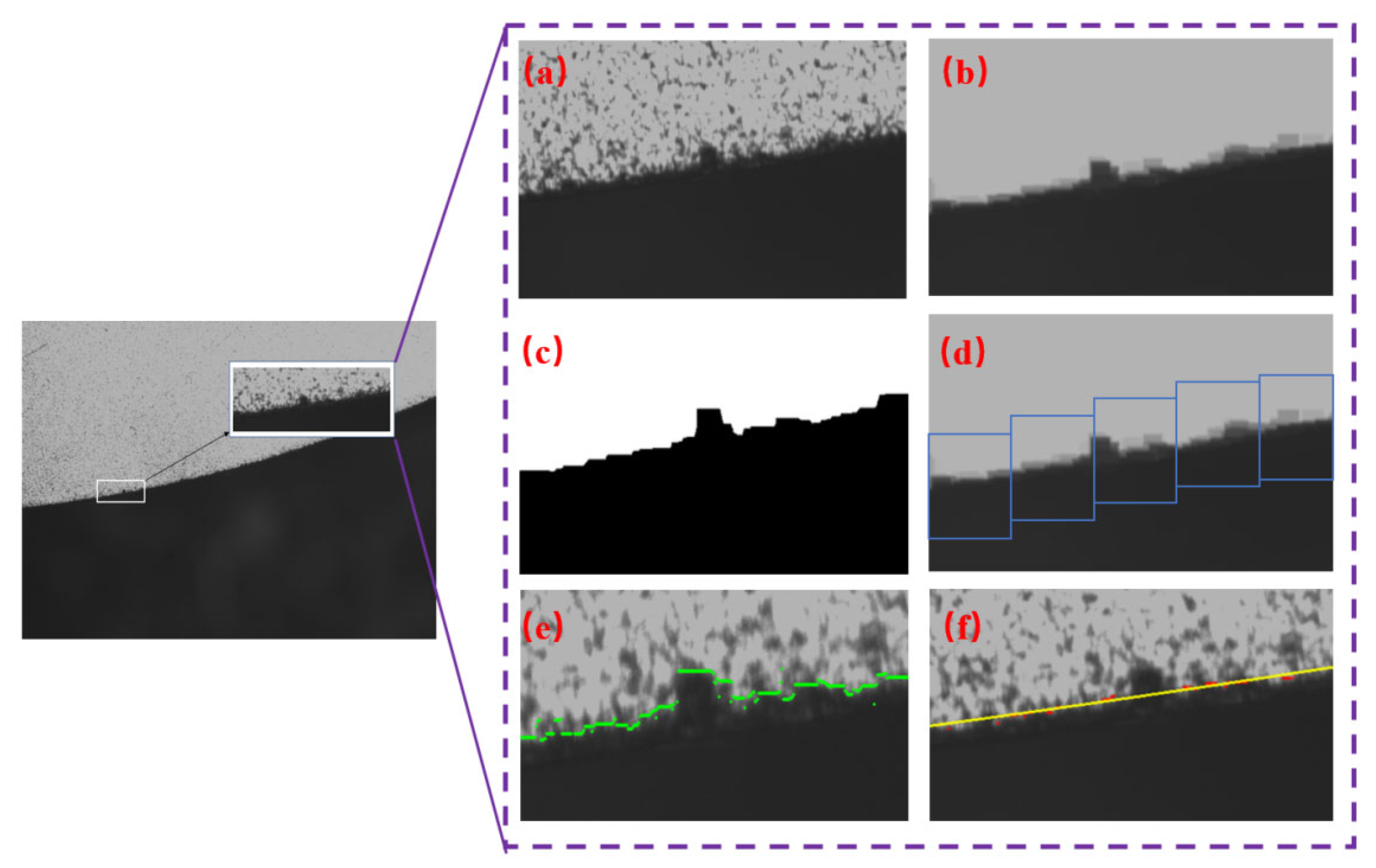
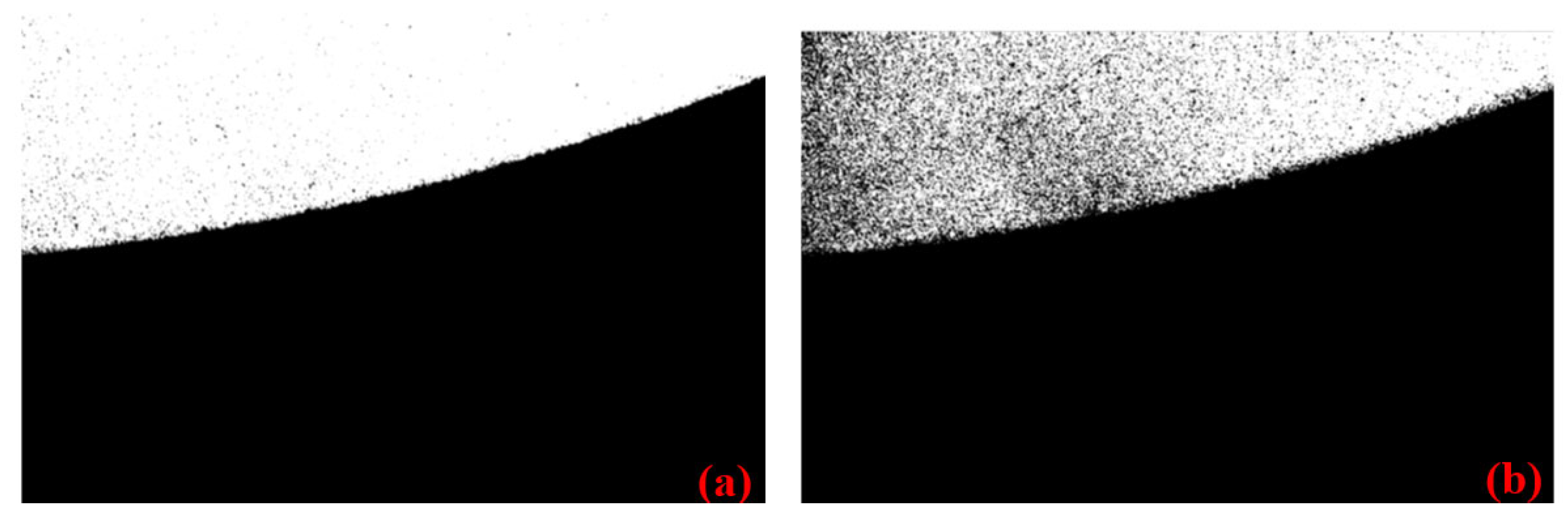
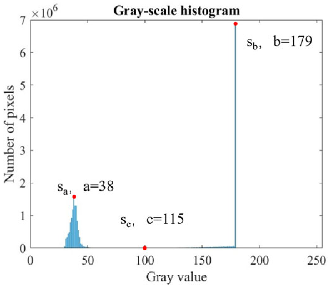
- The vision module, based on CNC servo feedback, resolves the trade-off between field of view and precision. By integrating peak detection, an improved Canny algorithm, and edge fitting techniques, the method achieves a repeatable localization accuracy better than 5 μm/0.005° in the X, Y, and C directions.
- (3)
- The probe module collects 3D coordinate data, and polynomial-based equidistant surface fitting is used to compensate for the ball tip radius. A stepwise global optimization model is constructed by combining a synchronous iterative localization algorithm with the NSGA-II multi-objective optimization algorithm. The simulation results show that for curved workpieces, only nine measurement points (25 in reference [31]) are needed to achieve a positioning accuracy better than 10 μm/0.01°.
- (4)
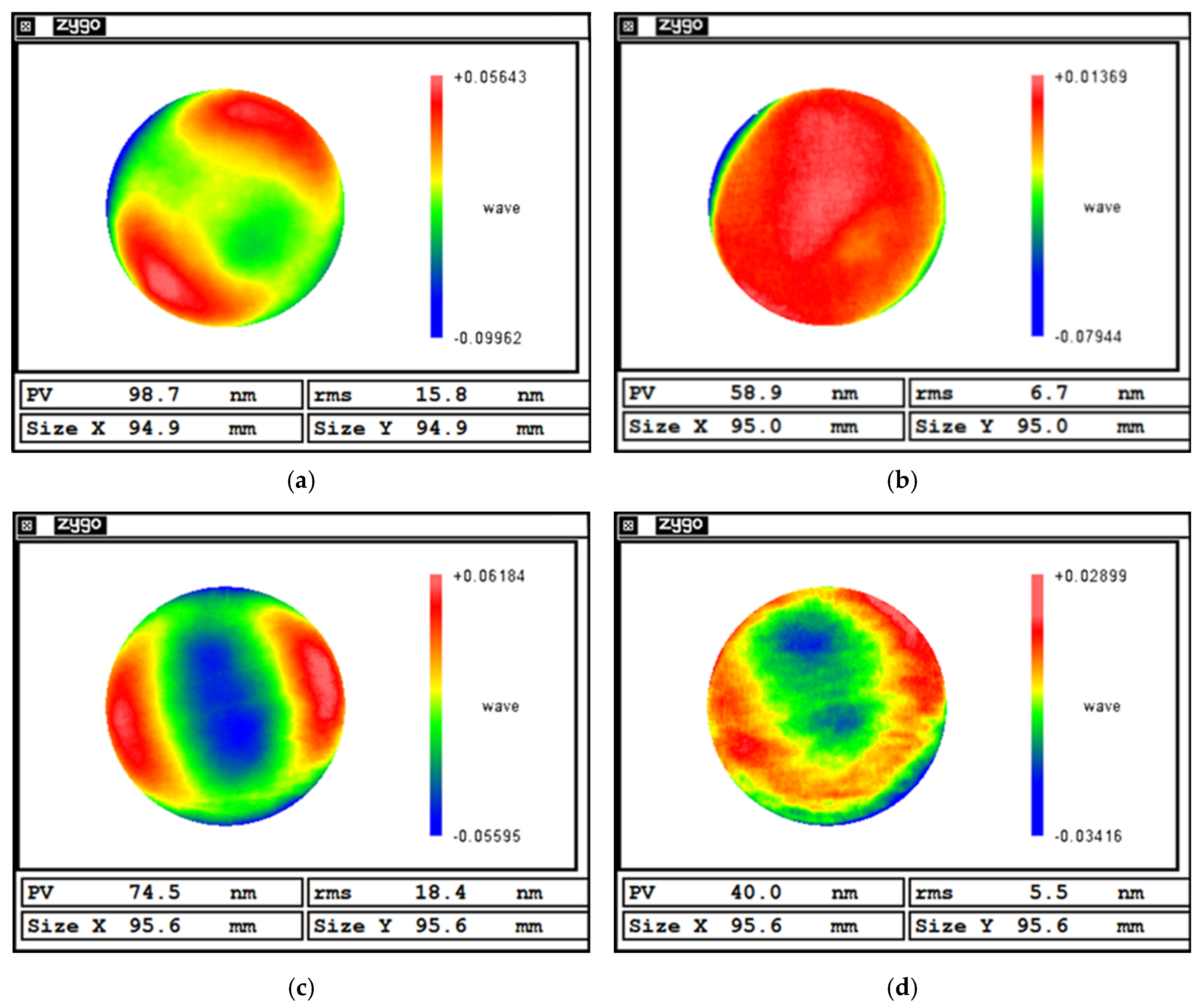
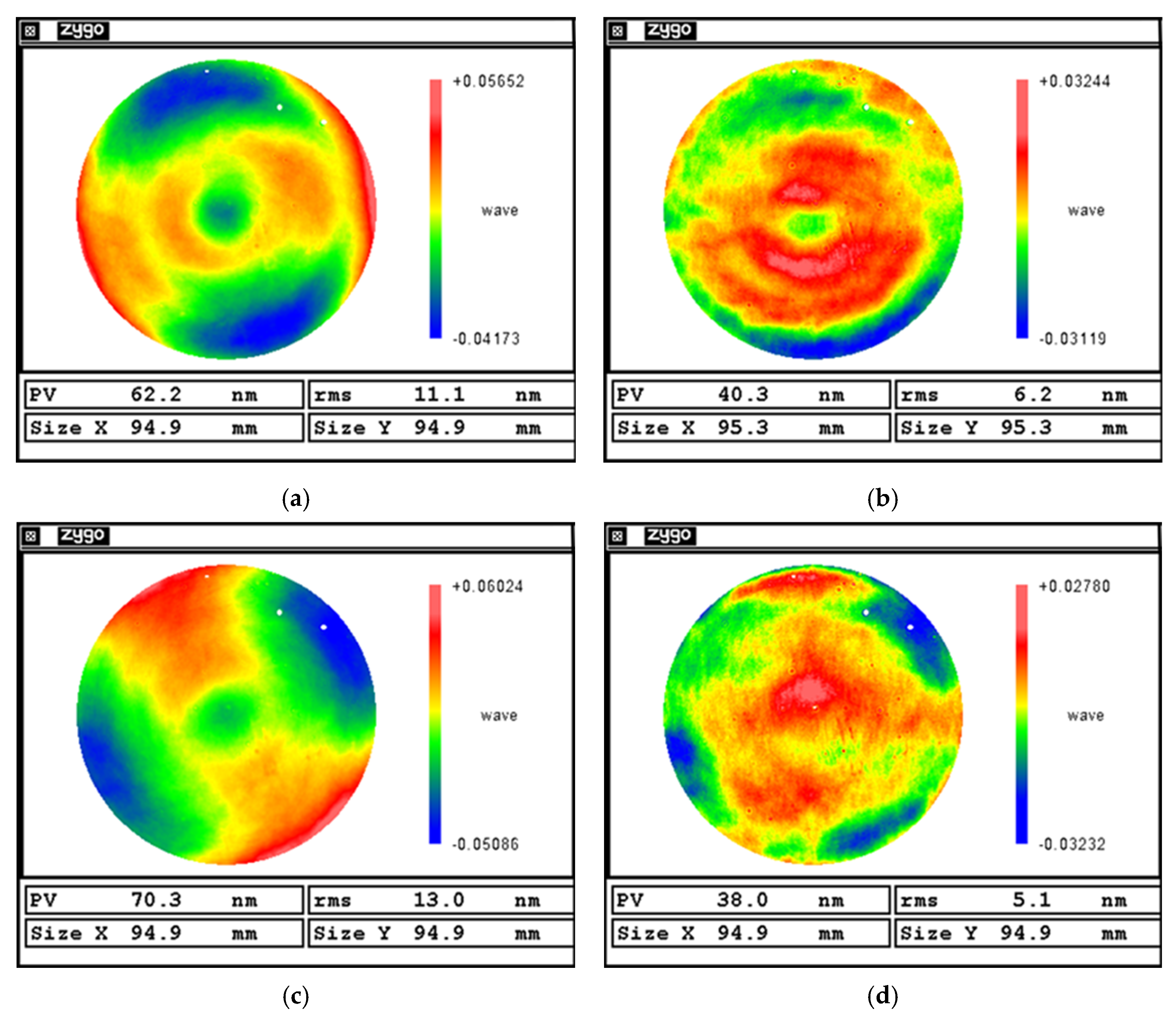
- The experimental results demonstrate that, compared to traditional alignment, the proposed self-positioning method improves the convergence ratio by 41.9% for planar workpieces and reduces the setup time by 66.7%. For the curved workpiece, the convergence ratio increases by 25.7%, with an 80% reduction in the alignment time.
Author Contributions
Funding
Data Availability Statement
Conflicts of Interest
References
- Li, J.; He, J.; Peng, Y. Development analysis of magnetorheological precession finishing (MRPF) technology. Opt. Express 2023, 31, 43535–43549. [Google Scholar] [CrossRef] [PubMed]
- Angel, J. Very large ground-based telescopes for optical and IR astronomy. Nature 1982, 295, 651–657. [Google Scholar] [CrossRef]
- Levinson, H. The Era of High-NA EUV Lithography Has Arrived! J. Micro Nanopatterning Mater. Metrol. 2025, 24, 010101. [Google Scholar] [CrossRef]
- He, T.; Wei, C.; Jiang, Z.; Zhao, Y.; Shao, J. Super-smooth surface demonstration and the physical mechanism of CO2 laser polishing of fused silica. Opt. Lett. 2018, 43, 5777–5780. [Google Scholar] [CrossRef] [PubMed]
- Hu, J.; Hu, H.; Peng, X.; Wang, Y.; Xue, S.; Liu, Y.; Du, C. Multi-dimensional error figuring model for ion beams in X-ray mirrors. Opt. Express 2024, 32, 29458–29473. [Google Scholar] [CrossRef] [PubMed]
- Dai, Y.; Hu, H.; Peng, X.; Wang, J.; Shi, F. Research on error control and compensation in magnetorheological finishing. Appl. Opt. 2011, 50, 3321–3329. [Google Scholar] [CrossRef]
- Chen, C.; Dai, Y.; Hu, H.; Guan, C. Study on the influence of a magnetorheological finishing path on the mid-frequency errors of optical element surfaces. Opt. Express 2024, 32, 19133–19145. [Google Scholar] [CrossRef]
- Shi, F.; Tie, G.; Zhang, W.; Song, C.; Tian, Y.; Shen, Y.; Wang, B. The Cause of Ribbon Fluctuation in Magnetorheological Finishing and Its Influence on Surface Mid-Spatial Frequency Error. Micromachines 2022, 13, 697. [Google Scholar] [CrossRef]
- Zhang, L.; Wan, S.; Li, H.; Guo, H.; Wei, C.; Zhang, D.; Shao, J. Modeling and in-depth analysis of the mid-spatial-frequency error influenced by actual contact pressure distribution in sub-aperture polishing. Opt. Express 2023, 31, 14414–14431. [Google Scholar] [CrossRef]
- Liu, S.; Wang, H.; Hou, J.; Zhang, Q.; Zhong, B.; Chen, X.; Zhang, M. Morphology characterization of polishing spot and process parameters optimization in magnetorheological finishing. J. Manuf. Process. 2022, 80, 259–272. [Google Scholar] [CrossRef]
- Wang, B.; Tie, G.; Shi, F.; Song, C.; Guo, S. Research on the influence of the non-stationary effect of the magnetorheological finishing removal function on mid-frequency errors of optical component surfaces. Opt. Express 2023, 31, 35016–35031. [Google Scholar] [CrossRef] [PubMed]
- Schinhaerl, M.; Smith, G.; Stamp, R.; Rascher, R.; Smith, L.; Pitschke, E.; Sperber, P.; Geiss, A. Mathematical modelling of influence functions in computer-controlled polishing: Part II. Appl. Math. Model. 2008, 32, 2907–2924. [Google Scholar] [CrossRef]
- Dai, Y.; Song, C.; Peng, X.; Shi, F. Calibration and prediction of removal function in magnetorheological finishing. Appl. Opt. 2010, 49, 298–306. [Google Scholar] [CrossRef]
- Liu, J.; Huang, P.; Peng, Y. Research on the tool influence function characteristics of magnetorheological precession finishing (MRPF). Opt. Express 2024, 32, 12537–12550. [Google Scholar] [CrossRef]
- Liu, J.; Li, X.; Zhang, Y.; Tian, D.; Ye, M.; Wang, C. Predicting the material removal rate (MRR) in surface magnetorheological finishing (MRF) based on the synergistic effect of pressure and shear stress. Appl. Surf. Sci. 2020, 504, 144492. [Google Scholar] [CrossRef]
- Yan, K.; Li, L.; Cheng, R.; Liu, X.; Li, X.; Bai, Y.; Zhang, X. Mapping model of ribbon contour and tool influence function based on distributed parallel neural networks in magneto-rheological finishing. Opt. Express 2024, 32, 27099–27111. [Google Scholar] [CrossRef] [PubMed]
- Hu, H.; Dai, Y.; Peng, X.; Wang, J. Research on reducing the edge effect in magnetorheological finishing. Appl. Opt. 2011, 50, 1220–1226. [Google Scholar] [CrossRef]
- Tang, C.; Yan, H.; Luo, Z.; Zhang, Y.; Wen, S. High precision edge extrapolation technique in continuous phase plate magnetorheological polishing. Infrared Laser Eng. 2019, 48, 442001. [Google Scholar] [CrossRef]
- Jeon, M.; Jeong, S.; Kang, J.; Yeo, W.; Kim, Y.; Choi, H.; Lee, W. Prediction model for edge effects in magnetorheological finishing based on edge tool influence function. Int. J. Precis. Eng. Manuf. 2022, 23, 1275–1289. [Google Scholar] [CrossRef]
- Hu, H.; Dai, Y.; Peng, X. Restraint of tool path ripple based on surface error distribution and process parameters in deterministic finishing. Opt. Express 2010, 18, 22973–22981. [Google Scholar] [CrossRef]
- Wang, T.; Cheng, H.; Zhang, W.; Yang, H.; Wu, W. Restraint of path effect on optical surface in magnetorheological jet polishing. Appl. Opt. 2016, 55, 935–942. [Google Scholar] [CrossRef] [PubMed]
- Wang, C.; Wang, Z.; Xu, Q. Unicursal random maze tool path for computer-controlled optical surfacing. Appl. Opt. 2015, 54, 10128–10136. [Google Scholar] [CrossRef] [PubMed]
- Zhao, Q.; Zhang, L.; Fan, C. Six-directional pseudorandom consecutive unicursal polishing path for suppressing mid-spatial frequency error and realizing consecutive uniform coverage. Appl. Opt. 2019, 58, 8529–8541. [Google Scholar] [CrossRef]
- Wan, S.; Wei, C.; Hu, C.; Situ, G.; Shao, Y.; Shao, J. Novel magic angle-step state and mechanism for restraining the path ripple of magnetorheological finishing. Int. J. Mach. Tools Manuf. 2021, 161, 103673. [Google Scholar] [CrossRef]
- Gao, B.; Fan, B.; Wang, J.; Wu, X.; Xin, Q. A Method for Optimizing the Dwell Time of Optical Components in Magnetorheological Finishing Based on Particle Swarm Optimization. Micromachines 2023, 15, 18. [Google Scholar] [CrossRef]
- Kang, H.; Wang, T.; Choi, H.; Kim, D. Genetic algorithm-powered non-sequential dwell time optimization for large optics fabrication. Opt. Express 2022, 30, 16442–16458. [Google Scholar] [CrossRef] [PubMed]
- Li, L.; Zheng, L.; Deng, W.; Wang, X.; Wang, X.; Zhang, B.; Bai, Y.; Hu, H.; Zhang, X. Optimized dwell time algorithm in magnetorheological finishing. Int. J. Adv. Manuf. Technol. 2015, 81, 833–841. [Google Scholar] [CrossRef]
- Zhang, Y.; Fang, F.; Huang, W.; Fan, W. Dwell time algorithm based on bounded constrained least squares under dynamic performance constraints of machine tool in deterministic optical finishing. Int. J. Precis. Eng. Manuf.-Green Technol. 2021, 8, 1415–1427. [Google Scholar] [CrossRef]
- Zhou, T.; Huang, W.; Chen, H.; Zhang, Y.; Zheng, Y.; Fan, W. Precise localization of square workpiece in magnetorheological polishing based on ICP algorithm. Manuf. Technol. Mach. Tool 2019, 7, 43–47. (In Chinese) [Google Scholar]
- Zhou, T.; Zhang, Y.; Fan, W.; Huang, W.; Zhang, J. Precise localization of rotary symmetrical aspheric workpiece in magnetorheological polishing. Opt. Precis. Eng. 2020, 28, 610–620. (In Chinese) [Google Scholar] [CrossRef]
- Peng, X.; Yang, C.; Hu, H.; Dai, Y. Measurement and algorithm for localization of aspheric lens in magnetorheological finishing. Int. J. Adv. Manuf. Technol. 2017, 88, 2889–2897. [Google Scholar] [CrossRef]
- Chen, L.; Zhong, G.; Han, Z.; Li, Q.; Wang, Y.; Pan, H. Binocular visual dimension measurement method for rectangular workpiece with a precise stereoscopic matching algorithm. Meas. Sci. Technol. 2023, 34, 035010. [Google Scholar] [CrossRef]
- Shen, T.; Huang, J.; Menq, C. Multiple-sensor integration for rapid and high-precision coordinate metrology. IEEE/ASME Trans. Mechatron. 2000, 5, 110–121. [Google Scholar] [CrossRef]
- de Araujo, P.R.M.; Lins, R.G. Cloud-based approach for automatic CNC workpiece origin localization based on image analysis. Robot. Comput.-Integr. Manuf. 2021, 68, 102090. [Google Scholar] [CrossRef]
- Zhou, B.; Liu, Y.; Xiao, Y.; Zhou, R.; Gan, Y.; Fang, F. Intelligent guidance programming of welding robot for 3D curved welding seam. IEEE Access 2021, 9, 42345–42357. [Google Scholar] [CrossRef]
- Zhang, X.; Xu, M. In-situ deflectometric measurement of optical surfaces for precision manufacturing. Opto-Electron. Eng. 2020, 47, 70–79. (In Chinese) [Google Scholar]
- Lei, Y.M.; Qi, J. A method of vehicle dashboard image location based on machine vision. In Proceedings of the International Conference on Information Science and Control Engineering, Shanghai, China, 20–22 December 2019. [Google Scholar]
- Otsu, N. A Threshold Selection Method from Gray-Level Histograms. IEEE Trans. Syst. Man Cybern. 1979, 9, 62–66. [Google Scholar] [CrossRef]
- Zack, G.W.; Rogers, W.E.; Latt, S.A. Automatic measurement of sister chromatid exchange frequency. J. Histochem. Cytochem. 1977, 25, 741–753. [Google Scholar] [CrossRef] [PubMed]
- Felix, S.; Jens, B.; Martin, W. An efficient algorithm for automatic peak detection in noisy periodic and quasi-periodic signals. Algorithms 2012, 5, 588–603. [Google Scholar] [CrossRef]
- Canny, J. A Computational Approach to Edge Detection. IEEE Trans. Pattern Anal. Mach. Intell. 1986, 8, 679–698. [Google Scholar] [CrossRef]
- Xiong, Z.; Li, Z. Probe radius compensation of workpiece localization. J. Manuf. Sci. Eng. 2003, 125, 100–104. [Google Scholar] [CrossRef]
- Brockett, R. Least squares matching problems. Linear Algebra Its Appl. 1989, 122, 761–777. [Google Scholar] [CrossRef]
- Paul, B.; McKay, N.D. A Method for Registration of 3-D Shapes. Proc. SPIE-Int. Soc. Opt. Eng. 1992, 14, 239–256. [Google Scholar]
- Yi, X.; Ma, L.; Li, Z. Geometric algorithms for workpiece localization. IEEE Trans. Robot. Autom. 1998, 14, 864–878. [Google Scholar]
- Deb, K.; Pratap, A.; Agarwal, S.; Meyarivan, T. A fast and elitist multiobjective genetic algorithm: NSGA-II. IEEE Trans. Evol. Comput. 2002, 2, 182–197. [Google Scholar] [CrossRef]


| Parameter | Value |
|---|---|
| Polishing wheel speed (rpm) | 200 |
| Magnetic field current (A) | 6.5 |
| Flow rate (L/h) | 100 |
| Indentation depth (mm) | 0.18/0.2/0.22/0.23/0.24/0.245/0.250/0.255/0.260/0.27/0.28/0.3/0.32 |
| Direction | Magnitude | ||||||||||
|---|---|---|---|---|---|---|---|---|---|---|---|
| X/mm | 0.005 | 0.01 | 0.015 | 0.02 | 0.025 | 0.03 | 0.04 | 0.05 | 0.06 | 0.08 | 0.1 |
| Z/mm | 0.005 | 0.01 | 0.015 | 0.02 | 0.025 | 0.03 | 0.04 | 0.05 | 0.06 | 0.08 | 0.1 |
| A/° | 0.005 | 0.01 | 0.015 | 0.04 | 0.05 | 0.06 | 0.08 | 0.1 | 0.12 | 0.16 | 0.2 |
| Combined | X = 0.01 mm, Y = 0.01 mm, Z = 0.005 mm, A = 0.005°, B = 0.005° | ||||||||||
| Component | Specification |
|---|---|
| Camera (A3B00MG000, iRAYPLE, Hangzhou, China) | Resolution: 5472 × 3648; pixel size: 2.4 μm |
| Lens (CR-XF-10MDT05X220D-1C, Shenzhen Can-Rill Technologies, Shenzhen, China) | Focal length: 220 mm; optical magnification: 0.5× |
| Cylinder (FESTO-DSM-12-270-P-A-B, Festo AG & Co. KG, Esslingen, Germany) | Working pressure: 0.2–1 MPa |
| Probe (Renishaw-LP2, RENISHAW, Wotton Under Edge, UK) | Trigger force: 5.85 N; repeatability: 1 μm |
| Parameter Name | Value |
|---|---|
| Aperture (mm) | 100 |
| R(mm) | 1065.36 |
| K | −2.18 |
| Category | Combined Error (σ) | |
|---|---|---|
| Probe data acquisition | Machine tool motion error (3 μm) | 2.45 um |
| Probe triggering error (1.5 μm) | ||
| Workpiece form error (10 μm) | ||
| Vision-based localization error | 1.23 um | |
| Offset Setting | g = [50, 10, 8, 10, 6, 0] | |g − g| = [0, 0, 0, 0, 0, 0] |
|---|---|---|
| After initial optimization | g1 = [49.989, 10.007, 8.002, 10.003, 6.001, 0] | |g − g1| = [0.011, 0.007, 0.002, 0.003, 0.001, 0] |
| After global optimization | g2 = [49.999, 10.006, 8.003, 10.001, 6.002, 0] | |g − g2| = [0.001, 0.006, 0.003, 0.001, 0.002, 0] |
| Type | Aperture (mm) | Radius of Curvature (mm) | Material | Mechanical Properties of Materials |
|---|---|---|---|---|
| Planar | 100 | Fused Silica | Mohs hardness: 7 Thermal expansion coefficient: 0.5 × 10⁻⁶/°C Dense amorphous SiO2 structure | |
| Spherical | 100 | 400 |
| Before Polishing | After Polishing | Convergence Ratio | Time/min | ||||
|---|---|---|---|---|---|---|---|
| PV/nm | RMS/nm | PV/nm | RMS/nm | PV/nm | RMS/nm | ||
| Traditional alignment | 98.7 | 15.8 | 58.9 | 6.7 | 1.68 | 2.36 | ~30 |
| Self-positioning | 74.5 | 18.4 | 40.0 | 5.5 | 1.86 | 3.35 | ~10 |
| Before Polishing | After Polishing | Convergence Ratio | Time/min | ||||
|---|---|---|---|---|---|---|---|
| PV/nm | RMS/nm | PV/nm | RMS/nm | PV/nm | RMS/nm | ||
| Traditional alignment | 62.2 | 11.1 | 40.3 | 6.2 | 1.54 | 1.79 | ~50 |
| Self-positioning | 70.3 | 13.0 | 38.0 | 5.1 | 1.85 | 2.55 | ~10 |
Disclaimer/Publisher’s Note: The statements, opinions and data contained in all publications are solely those of the individual author(s) and contributor(s) and not of MDPI and/or the editor(s). MDPI and/or the editor(s) disclaim responsibility for any injury to people or property resulting from any ideas, methods, instructions or products referred to in the content. |
© 2025 by the authors. Licensee MDPI, Basel, Switzerland. This article is an open access article distributed under the terms and conditions of the Creative Commons Attribution (CC BY) license (https://creativecommons.org/licenses/by/4.0/).
Share and Cite
Zhang, Y.; Wang, P.; Guan, C.; Liu, M.; Peng, X.; Hu, H. A Novel High-Precision Workpiece Self-Positioning Method for Improving the Convergence Ratio of Optical Components in Magnetorheological Finishing. Micromachines 2025, 16, 730. https://doi.org/10.3390/mi16070730
Zhang Y, Wang P, Guan C, Liu M, Peng X, Hu H. A Novel High-Precision Workpiece Self-Positioning Method for Improving the Convergence Ratio of Optical Components in Magnetorheological Finishing. Micromachines. 2025; 16(7):730. https://doi.org/10.3390/mi16070730
Chicago/Turabian StyleZhang, Yiang, Pengxiang Wang, Chaoliang Guan, Meng Liu, Xiaoqiang Peng, and Hao Hu. 2025. "A Novel High-Precision Workpiece Self-Positioning Method for Improving the Convergence Ratio of Optical Components in Magnetorheological Finishing" Micromachines 16, no. 7: 730. https://doi.org/10.3390/mi16070730
APA StyleZhang, Y., Wang, P., Guan, C., Liu, M., Peng, X., & Hu, H. (2025). A Novel High-Precision Workpiece Self-Positioning Method for Improving the Convergence Ratio of Optical Components in Magnetorheological Finishing. Micromachines, 16(7), 730. https://doi.org/10.3390/mi16070730