
Cosserat Rod-Based Tendon Friction Modeling, Simulation, and Experiments for Tendon-Driven Continuum Robots

Abstract
1. Introduction
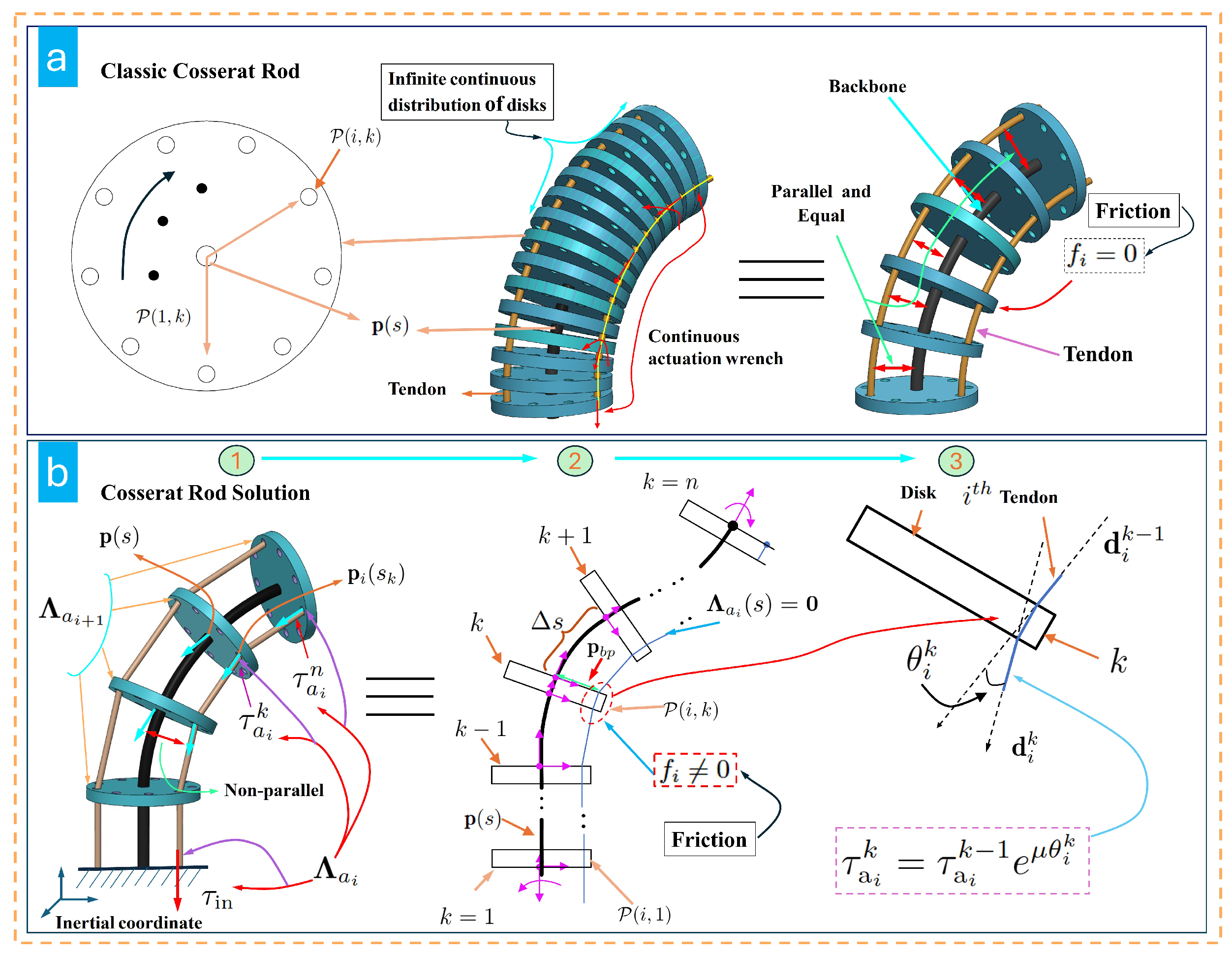
2. Modeling
2.1. Cosserat Rod Model
2.2. Methodological Contributions
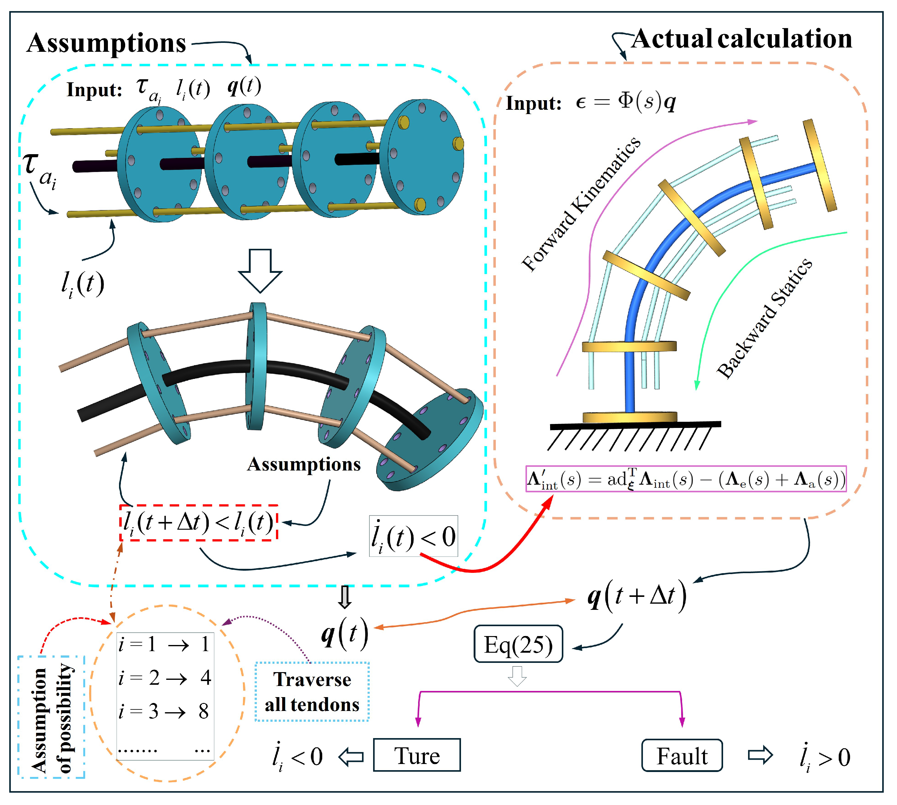
2.3. Discrete Tendon TDCR Model Without Friction
2.4. Discrete TDCR Model Considering Friction
3. Numerical Simulation and Experiment
3.1. Numerical Simulation
3.2. Experimental System
3.3. Experimental Procedures
3.4. TDCR Parameter Identification
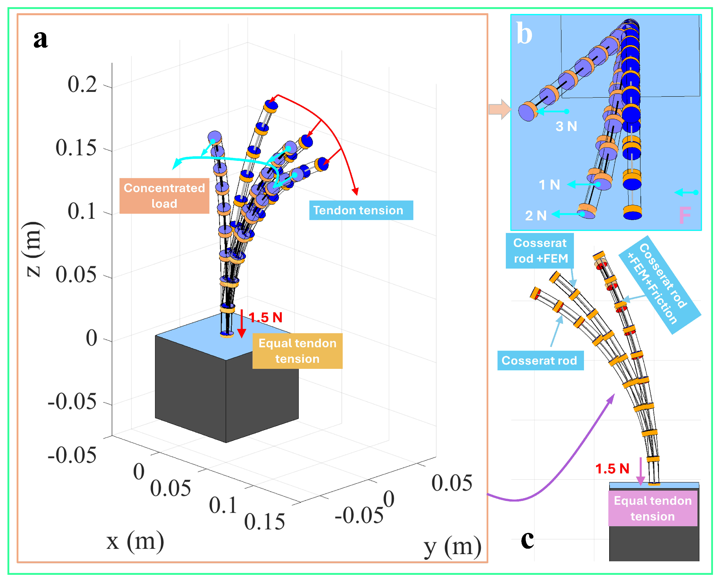
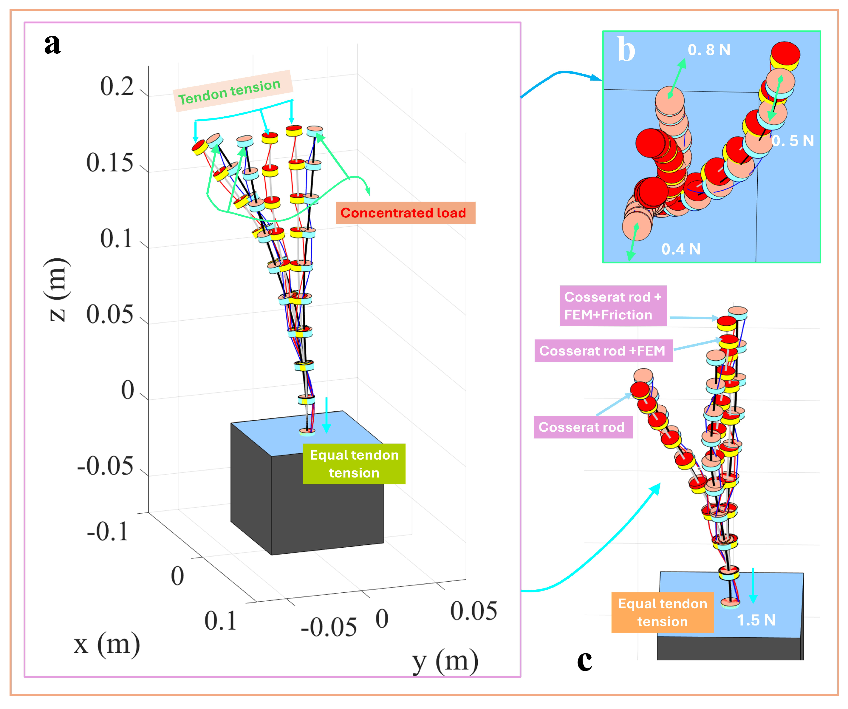
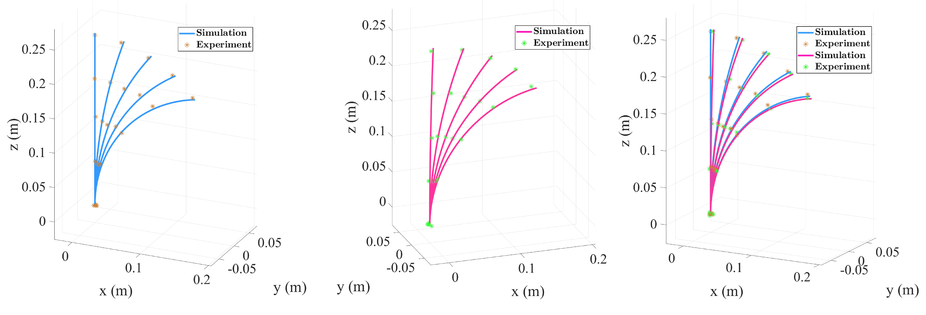
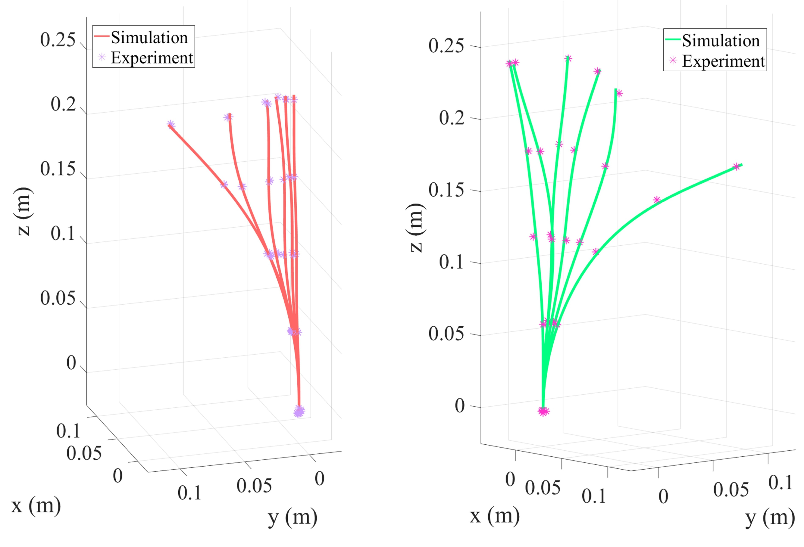
3.5. Single-Segment Collinear Tendon Routing
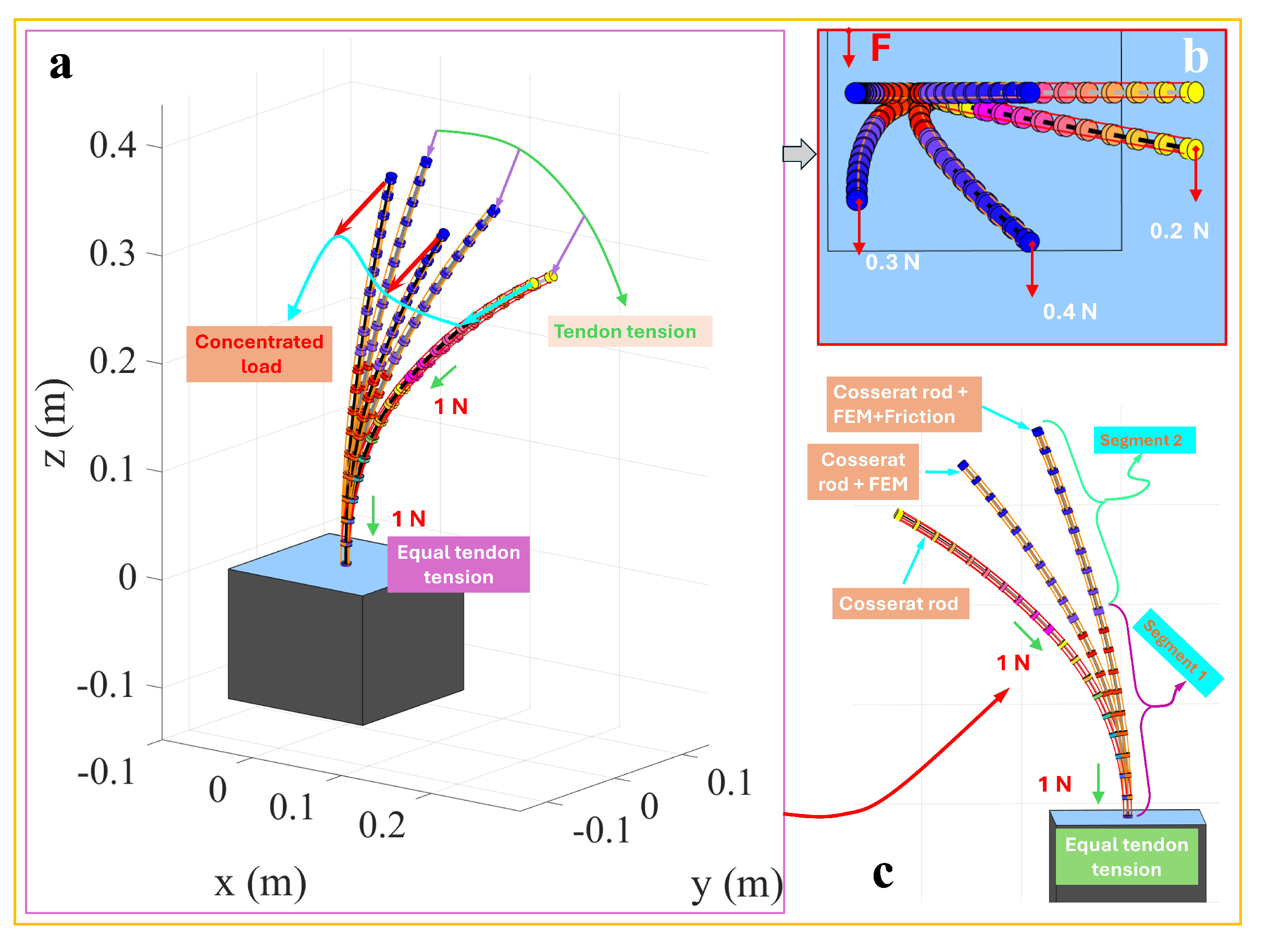
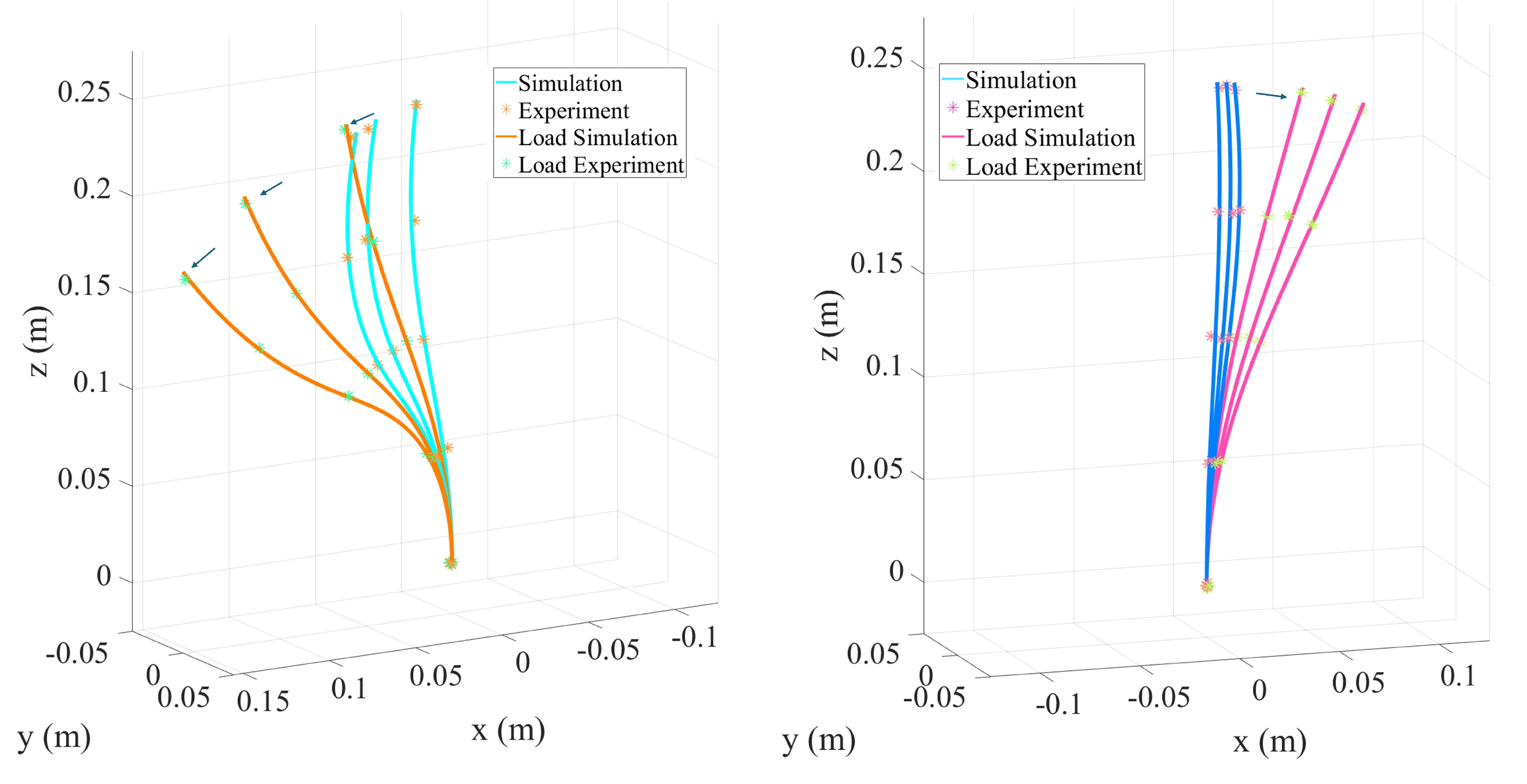
3.6. Two-Segment Collinear Tendon Routing
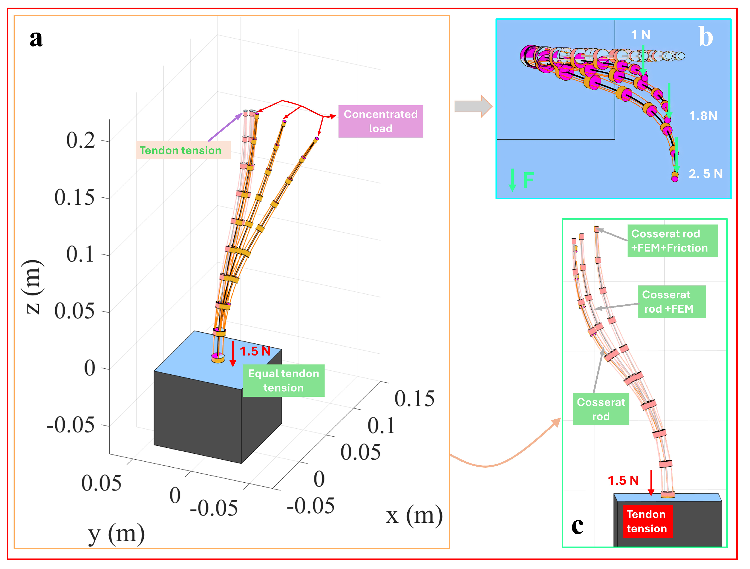
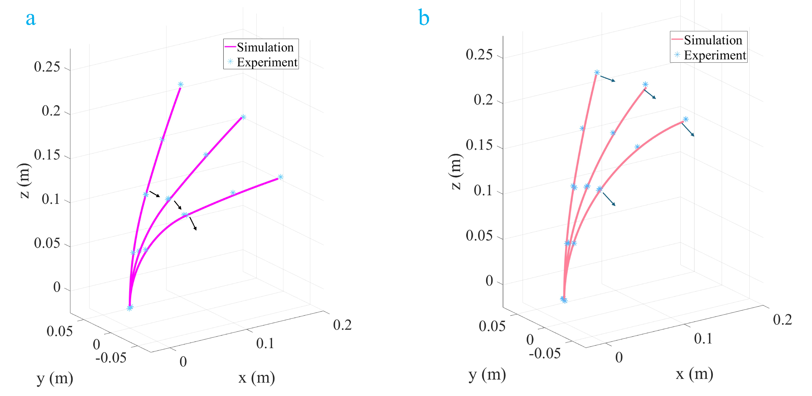
3.7. Helical Tendon Routing
3.8. Converging Tendon Routing
4. Discussion
5. Conclusions
Author Contributions
Funding
Data Availability Statement
Acknowledgments
Conflicts of Interest
References
- Wang, H.; Mao, Y.; Du, J. Continuum Robots and Magnetic Soft Robots: From Models to Interdisciplinary Challenges for Medical Applications. Micromachines 2024, 15, 313. [Google Scholar] [CrossRef] [PubMed]
- Dupont, P.E.; Nelson, B.J.; Goldfarb, M.; Hannaford, B.; Menciassi, A.; O’Malley, M.K.; Simaan, N.; Valdastri, P.; Yang, G.Z. A decade retrospective of medical robotics research from 2010 to 2020. Sci. Robot. 2021, 6, eabi8017. [Google Scholar] [CrossRef] [PubMed]
- Burgner-Kahrs, J.; Rucker, D.C.; Choset, H. Continuum robots for medical applications: A survey. IEEE Trans. Robot. 2015, 31, 1261–1280. [Google Scholar] [CrossRef]
- Dong, X.; Wang, M.; Mohammad, A.; Ba, W.; Russo, M.; Norton, A.; Kell, J.; Axinte, D. Continuum robots collaborate for safe manipulation of high-temperature flame to enable repairs in challenging environments. IEEE/ASME Trans. Mechatron. 2022, 27, 4217–4220. [Google Scholar] [CrossRef]
- Wang, M.; Dong, X.; Ba, W.; Mohammad, A.; Axinte, D.; Norton, A. Design, modelling and validation of a novel extra slender continuum robot for in-situ inspection and repair in aeroengine. Robot. Comput.-Integr. Manuf. 2021, 67, 102054. [Google Scholar] [CrossRef]
- Dong, X.; Palmer, D.; Axinte, D.; Kell, J. In-situ repair/maintenance with a continuum robotic machine tool in confined space. J. Manuf. Process. 2019, 38, 313–318. [Google Scholar] [CrossRef]
- Jinzhao, Y.; Haijun, P.; Zhang, J.; Zhigang, W. Dynamic modeling and beating phenomenon analysis of space robots with continuum manipulators. Chin. J. Aeronaut. 2022, 35, 226–241. [Google Scholar]
- Yuan, H.; Li, Z. Workspace analysis of cable-driven continuum manipulators based on static model. Robot. Comput.-Integr. Manuf. 2018, 49, 240–252. [Google Scholar] [CrossRef]
- Wu, K.; Zheng, G. A comprehensive static modeling methodology via beam theory for compliant mechanisms. Mech. Mach. Theory 2022, 169, 104598. [Google Scholar] [CrossRef]
- Yang, J.; Peng, H.; Zhou, W.; Zhang, J.; Wu, Z. A modular approach for dynamic modeling of multisegment continuum robots. Mech. Mach. Theory 2021, 165, 104429. [Google Scholar] [CrossRef]
- Zhang, J.; Peng, H.; Zhou, W.; Yang, J.; Wu, Z. Dynamic Modeling and Verification of Continuum Robot Based on Cable Drive. In Proceedings of the 2019 IEEE 4th International Conference on Advanced Robotics and Mechatronics (ICARM), Toyonaka, Japan, 3–5 July 2019; pp. 262–267. [Google Scholar]
- Tian, Q.; Li, K.; Li, C. Dynamic Analysis of Cable-Driven Robot in the Framework of Absolute Node Coordinate Formulation. In Proceedings of the 2023 IEEE 7th International Conference on Electrical, Mechanical and Computer Engineering (ICEMCE), Xi’an, China, 20–22 October 2023; pp. 716–720. [Google Scholar]
- Sun, J.; Tian, Q.; Hu, H.; Pedersen, N.L. Axially variable-length solid element of absolute nodal coordinate formulation. Acta Mech. Sin. 2019, 35, 653–663. [Google Scholar] [CrossRef]
- Sun, J.; Tian, Q.; Hu, H.; Pedersen, N.L. Simultaneous topology and size optimization of a 3D variable-length structure described by the ALE–ANCF. Mech. Mach. Theory 2018, 129, 80–105. [Google Scholar] [CrossRef]
- Bai, Z.; Jiang, X.; Fu, X. Investigation of the retrieval dynamics of the tethered satellites using ANCF-ALE variable-length element. IEEE Trans. Aerosp. Electron. Syst. 2022, 59, 1980–1988. [Google Scholar] [CrossRef]
- Yang, S.; Ren, H.; Zhu, X. Dynamic modeling of cable deployment/retrieval based on ALE-ANCF and adaptive step-size integrator. Ocean Eng. 2024, 309, 118517. [Google Scholar] [CrossRef]
- Li, K.; Yu, Z.; Lan, P.; Tian, Q.; Lu, N. ALE-ANCF circular cross-section beam element and its application on the dynamic analysis of cable-driven mechanism. Multibody Syst. Dyn. 2024, 60, 417–446. [Google Scholar] [CrossRef]
- Alessi, C.; Agabiti, C.; Caradonna, D.; Laschi, C.; Renda, F.; Falotico, E. Rod models in continuum and soft robot control: A review. arXiv 2024, arXiv:2407.05886. [Google Scholar]
- Armanini, C.; Boyer, F.; Mathew, A.T.; Duriez, C.; Renda, F. Soft robots modeling: A structured overview. IEEE Trans. Robot. 2023, 39, 1728–1748. [Google Scholar] [CrossRef]
- Tummers, M.; Lebastard, V.; Boyer, F.; Troccaz, J.; Rosa, B.; Chikhaoui, M.T. Cosserat rod modeling of continuum robots from Newtonian and Lagrangian perspectives. IEEE Trans. Robot. 2023, 39, 2360–2378. [Google Scholar] [CrossRef]
- Rucker, D.C.; Webster, R.J., III. Statics and dynamics of continuum robots with general tendon routing and external loading. IEEE Trans. Robot. 2011, 27, 1033–1044. [Google Scholar] [CrossRef]
- Till, J.; Aloi, V.; Rucker, C. Real-time dynamics of soft and continuum robots based on Cosserat rod models. Int. J. Robot. Res. 2019, 38, 723–746. [Google Scholar] [CrossRef]
- Wu, G.; Shi, G. Design, modeling, and workspace analysis of an extensible rod-driven Parallel Continuum Robot. Mech. Mach. Theory 2022, 172, 104798. [Google Scholar] [CrossRef]
- Renda, F.; Giorelli, M.; Calisti, M.; Cianchetti, M.; Laschi, C. Dynamic model of a multibending soft robot arm driven by cables. IEEE Trans. Robot. 2014, 30, 1109–1122. [Google Scholar] [CrossRef]
- Renda, F.; Boyer, F.; Dias, J.; Seneviratne, L. Discrete cosserat approach for multisection soft manipulator dynamics. IEEE Trans. Robot. 2018, 34, 1518–1533. [Google Scholar] [CrossRef]
- Boyer, F.; Lebastard, V.; Candelier, F.; Renda, F. Dynamics of continuum and soft robots: A strain parameterization based approach. IEEE Trans. Robot. 2020, 37, 847–863. [Google Scholar] [CrossRef]
- Boyer, F.; Lebastard, V.; Candelier, F.; Renda, F.; Alamir, M. Statics and dynamics of continuum robots based on Cosserat rods and optimal control theories. IEEE Trans. Robot. 2022, 39, 1544–1562. [Google Scholar] [CrossRef]
- Briot, S.; Boyer, F. A Geometrically Exact Assumed Strain Modes Approach for the Geometrico-and Kinemato-Static Modelings of Continuum Parallel Robots. IEEE Trans. Robot. 2023, 39, 1527–1543. [Google Scholar] [CrossRef]
- Boyer, F.; Gotelli, A.; Tempel, P.; Lebastard, V.; Renda, F.; Briot, S. Implicit time integration simulation of robots with rigid bodies and Cosserat rods based on a Newton-Euler recursive algorithm. IEEE Trans. Robot. 2025, 41, 677–696. [Google Scholar] [CrossRef]
- Mathew, A.T.; Feliu-Talegon, D.; Alkayas, A.Y.; Boyer, F.; Renda, F. Reduced order modeling of hybrid soft-rigid robots using global, local, and state-dependent strain parameterization. Int. J. Robot. Res. 2024, 43, 02783649241262333. [Google Scholar] [CrossRef]
- Mathew, A.T.; Hmida, I.B.; Armanini, C.; Boyer, F.; Renda, F. A MATLAB toolbox for hybrid rigid soft robots based on the geometric variable strain approach. arXiv 2021, arXiv:2107.05494. [Google Scholar] [CrossRef]
- Li, H.; Xun, L.; Zheng, G. Piecewise linear strain Cosserat model for soft slender manipulator. IEEE Trans. Robot. 2023, 39, 2342–2359. [Google Scholar] [CrossRef]
- Li, H.; Xun, L.; Zheng, G.; Renda, F. Discrete Cosserat Static Model-Based Control of Soft Manipulator. IEEE Robot. Autom. Lett. 2023, 8, 1739–1746. [Google Scholar] [CrossRef]
- Li, H.; Xun, L.; Zheng, G. Global Control of Soft Manipulator by Unifying Cosserat and Neural Network. IEEE Trans. Ind. Electron. 2024, 71, 10944–10954. [Google Scholar] [CrossRef]
- Xun, L.; Zheng, G.; Kruszewski, A. Cosserat-rod based dynamic modeling of soft slender robot interacting with environment. IEEE Trans. Robot. 2024, 40, 2811–2830. [Google Scholar] [CrossRef]
- Yasin, R.; Simaan, N. Joint-level force sensing for indirect hybrid force/position control of continuum robots with friction. Int. J. Robot. Res. 2021, 40, 764–781. [Google Scholar] [CrossRef]
- Yuan, H.; Zhou, L.; Xu, W. A comprehensive static model of cable-driven multi-section continuum robots considering friction effect. Mech. Mach. Theory 2019, 135, 130–149. [Google Scholar] [CrossRef]
- Raimondi, L.; Russo, M.; Dong, X.; Axinte, D. Understanding friction and superelasticity in tendon-driven continuum robots. Mechatronics 2024, 104, 103241. [Google Scholar] [CrossRef]
- Liu, Z.; Zhang, X.; Cai, Z.; Peng, H.; Wu, Z. Real-time dynamics of cable-driven continuum robots considering the cable constraint and friction effect. IEEE Robot. Autom. Lett. 2021, 6, 6235–6242. [Google Scholar] [CrossRef]
- Feliu-Talegon, D.; Mathew, A.T.; Alkayas, A.Y.; Adamu, Y.A.; Renda, F. Dynamic shape estimation of tendon-driven soft manipulators via actuation readings. IEEE Robot. Autom. Lett. 2025, 10, 780–787. [Google Scholar] [CrossRef]
- Antman, S.S. Problems in nonlinear elasticity. In Nonlinear Problems of Elasticity; Springer: New York, NY, USA, 2005; pp. 1–835. [Google Scholar]
- Tasora, A.; Benatti, S.; Mangoni, D.; Garziera, R. A geometrically exact isogeometric beam for large displacements and contacts. Comput. Methods Appl. Mech. Eng. 2020, 358, 112635. [Google Scholar] [CrossRef]
- Epstein, M. The Geometrical Language of Continuum Mechanics; Cambridge University Press: Cambridge, UK, 2010. [Google Scholar]
- Renda, F.; Armanini, C.; Lebastard, V.; Candelier, F.; Boyer, F. A geometric variable-strain approach for static modeling of soft manipulators with tendon and fluidic actuation. IEEE Robot. Autom. Lett. 2020, 5, 4006–4013. [Google Scholar] [CrossRef]
- Jung, J.H.; Pan, N.; Kang, T.J. Capstan equation including bending rigidity and non-linear frictional behavior. Mech. Mach. Theory 2008, 43, 661–675. [Google Scholar] [CrossRef]


| Tension (N) | End Offset (mm) | End Bending Angle (°) | Load (N) | End Bending Angle Under Load (°) |
|---|---|---|---|---|
| 0.5 | 3.7 | 3.91 | 0.05 | 5.61 |
| 1 | 46.7 | 10.76 | 0.05 | 12.22 |
| 1.5 | 89.3 | 19.74 | 0.05 | 20.10 |
| 2 | 111.7 | 27.50 | 0.05 | 28.73 |
| 2.5 | 143.6 | 37.29 | 0.05 | 41.18 |
| Segment 1 | Segment 2 | End Offset (mm) | End Bending Angle (°) | Load (N) | |||
|---|---|---|---|---|---|---|---|
| Tension (N) | Tension (N) | Segment 1 | Segment 2 | Segment 1 | Segment 2 | Concentrated Load | End Load |
| 5 | 2 | 17.8 | 67.4 | 8.27 | 15.75 | 1 | 0 |
| 16 | 2 | 49.2 | 148.1 | 24.15 | 38.86 | 1 | 0 |
| 27 | 2 | 72.4 | 196.3 | 38.31 | 61.50 | 1 | 0 |
| 2 | 2 | 11.7 | 41.3 | 5.52 | 9.63 | 0.6 | 0.5 |
| 2 | 8 | 27.9 | 104.7 | 13.03 | 25.75 | 0.6 | 0.5 |
| 2 | 18 | 47.4 | 154.2 | 22.75 | 42.56 | 0.6 | 0.5 |
| Tendon Tension (N) | End Concentrated Load (N) | End Y-Axis Offset (mm) | End Bending Angle (°) | ||
|---|---|---|---|---|---|
| Applied Force | Applied Load | Without Load | With Load | Without Load | With Load |
| 5 | 0.8 | 4.3 | 20.7 | 0.99 | 5.50 |
| 10 | 0.8 | 10.8 | 37.4 | 2.48 | 9.43 |
| 15 | 0.8 | 16.3 | 17.3 | 3.86 | 10.25 |
| 20 | 0.8 | 24.6 | 17.2 | 5.69 | 4.89 |
| 25 | 0.8 | 53.7 | 100.6 | 12.66 | 26.67 |
| 30 | 0.8 | 86.2 | 85.4 | 24.79 | 39.06 |
| Tendon Force (N) | End Offset in x-Direction (mm) | End Bending Angle in x-Direction (°) | End Load (N) | ||
|---|---|---|---|---|---|
| Without Load | With Load | Without Load | With Load | ||
| 5 | 19.4 | 61.5 | 4.47 | 14.36 | 0.5 |
| 20 | 44.8 | 122.9 | 10.58 | 30.19 | 0.5 |
| 40 | 57.1 | 157.8 | 13.65 | 41.81 | 0.5 |
| 1 | 5.4 | 47.8 | 1.29 | 11.07 | 1 |
| 2 | 10.5 | 66 | 2.42 | 15.36 | 1 |
| 3 | 13.3 | 81.2 | 3.05 | 19.21 | 1 |
Disclaimer/Publisher’s Note: The statements, opinions and data contained in all publications are solely those of the individual author(s) and contributor(s) and not of MDPI and/or the editor(s). MDPI and/or the editor(s) disclaim responsibility for any injury to people or property resulting from any ideas, methods, instructions or products referred to in the content. |
© 2025 by the authors. Licensee MDPI, Basel, Switzerland. This article is an open access article distributed under the terms and conditions of the Creative Commons Attribution (CC BY) license (https://creativecommons.org/licenses/by/4.0/).
Share and Cite
Wang, H.; Du, J.; Mao, Y. Cosserat Rod-Based Tendon Friction Modeling, Simulation, and Experiments for Tendon-Driven Continuum Robots. Micromachines 2025, 16, 346. https://doi.org/10.3390/mi16030346
Wang H, Du J, Mao Y. Cosserat Rod-Based Tendon Friction Modeling, Simulation, and Experiments for Tendon-Driven Continuum Robots. Micromachines. 2025; 16(3):346. https://doi.org/10.3390/mi16030346
Chicago/Turabian StyleWang, Honghong, Jingli Du, and Yi Mao. 2025. "Cosserat Rod-Based Tendon Friction Modeling, Simulation, and Experiments for Tendon-Driven Continuum Robots" Micromachines 16, no. 3: 346. https://doi.org/10.3390/mi16030346
APA StyleWang, H., Du, J., & Mao, Y. (2025). Cosserat Rod-Based Tendon Friction Modeling, Simulation, and Experiments for Tendon-Driven Continuum Robots. Micromachines, 16(3), 346. https://doi.org/10.3390/mi16030346