
Comparison and Verification of Three Algorithms for Accuracy Improvement of Quartz Resonant Pressure Sensors

 , , ,
, , ,
Abstract
:1. Introduction
- Optimizing the geometry and topology of the sensor structure in order to limit the dependence of thermal expansion behavior on materials’ elastic property [8];
- Adding a composite structure (such as a SiO2 layer) to the resonator substrate to obtain an overall satisfactory temperature coefficient [9].
2. Materials and Methods
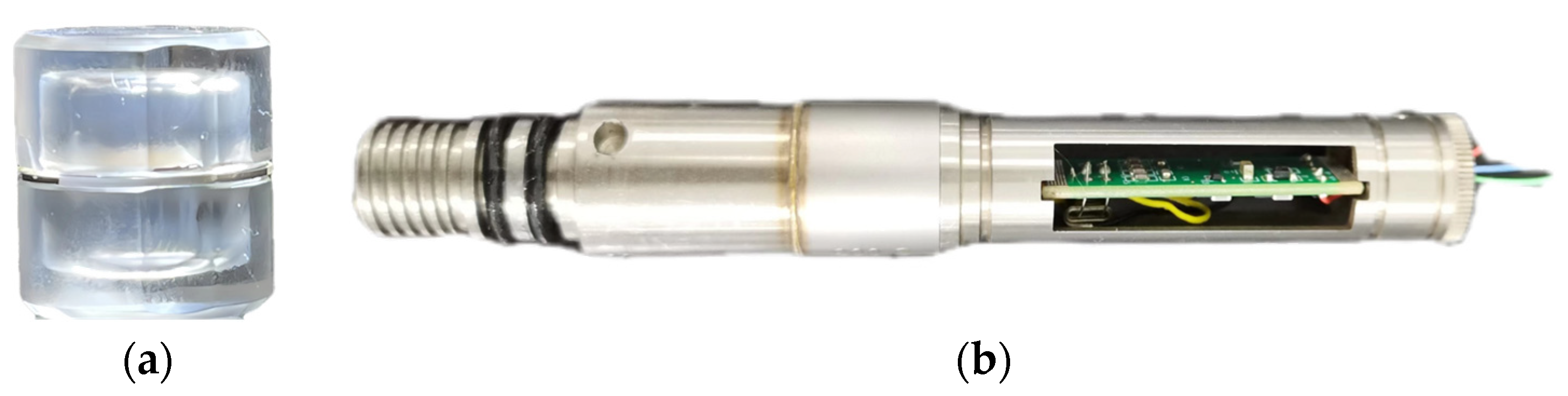
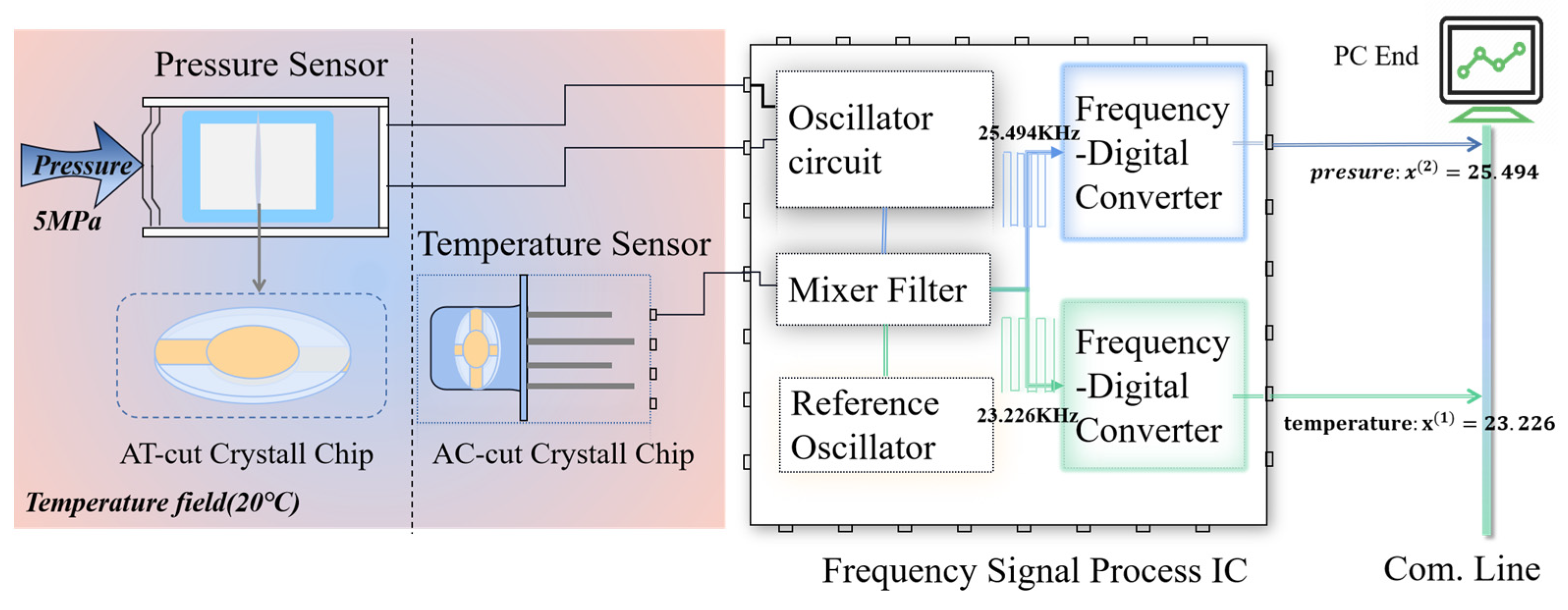
2.1. Quartz Resonant Pressure Sensor
2.2. Types of Regression Methods
2.2.1. Multivariate Polynomial Regression (MPR)
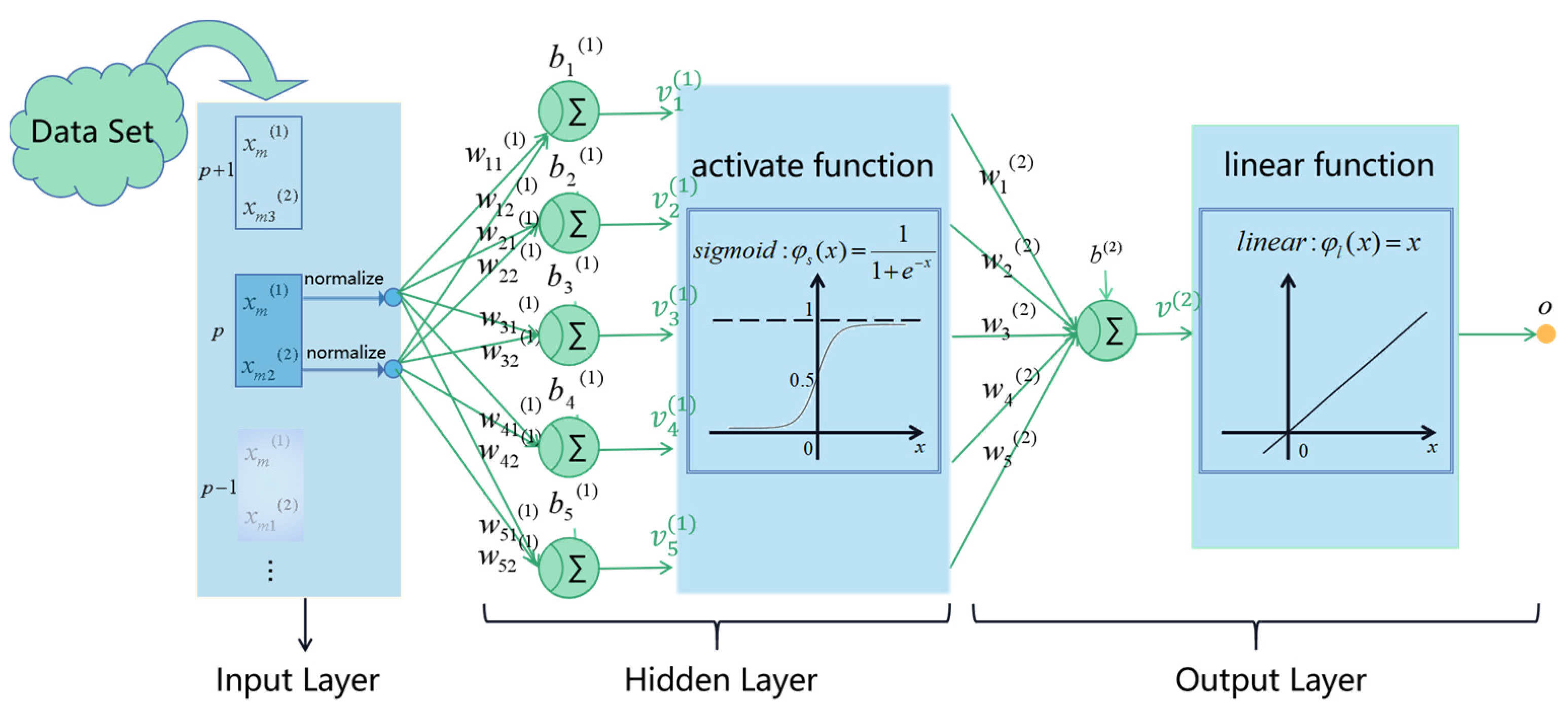
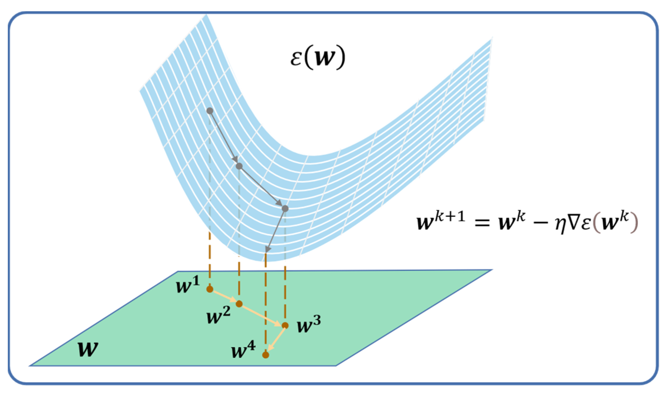
2.2.2. MLP
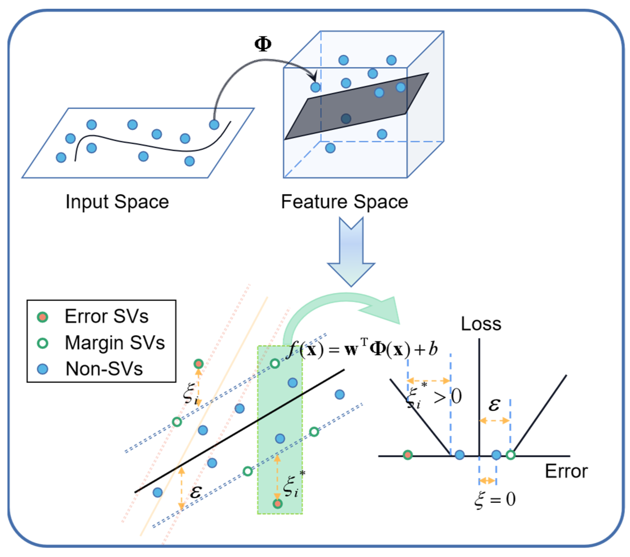
2.2.3. SVR
3. Results
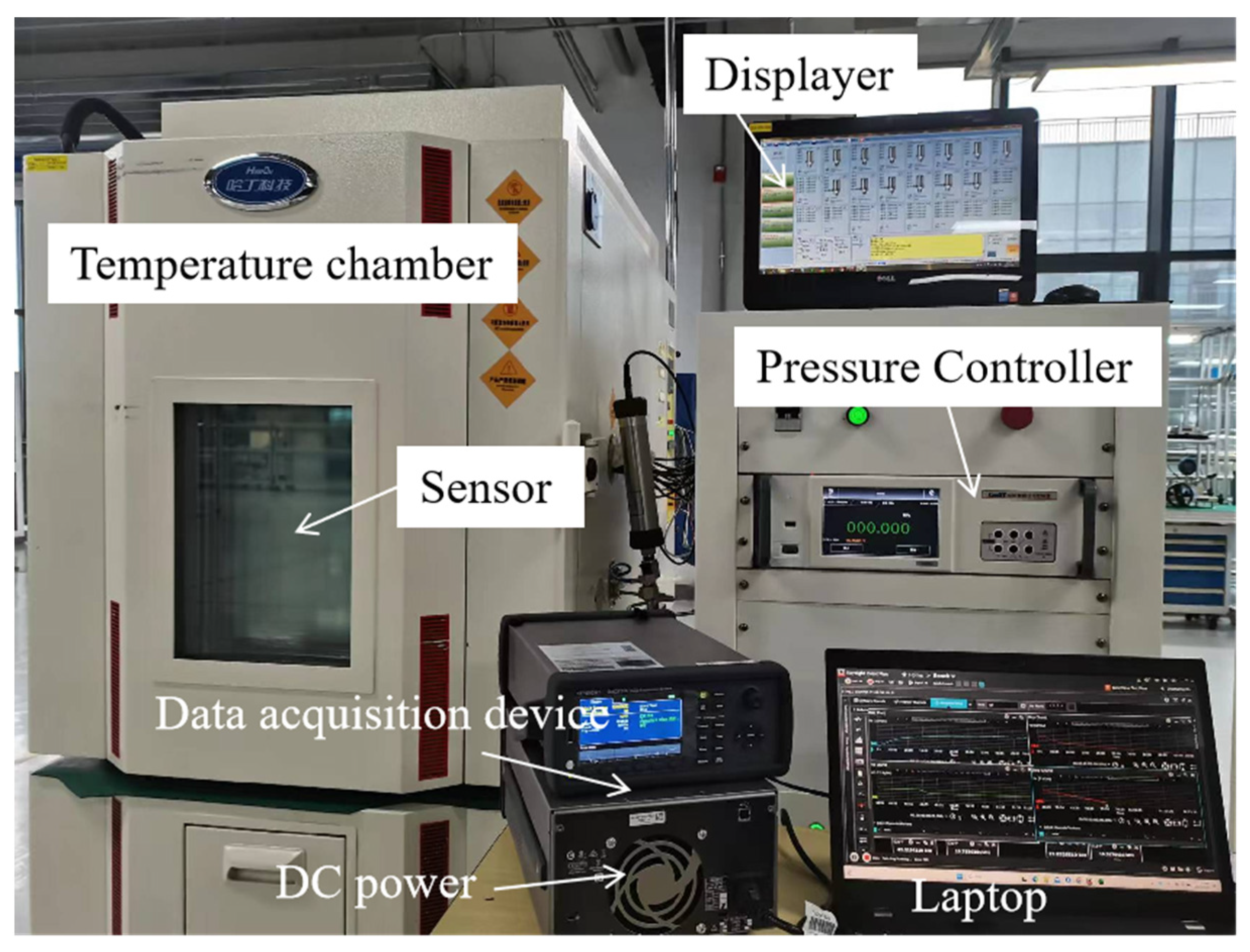
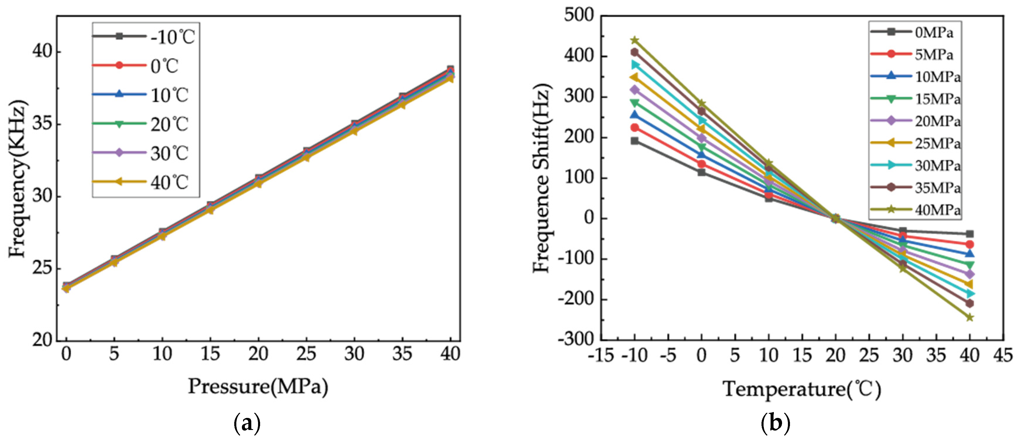
3.1. Calibration System and Performance Characteristics before Compensation
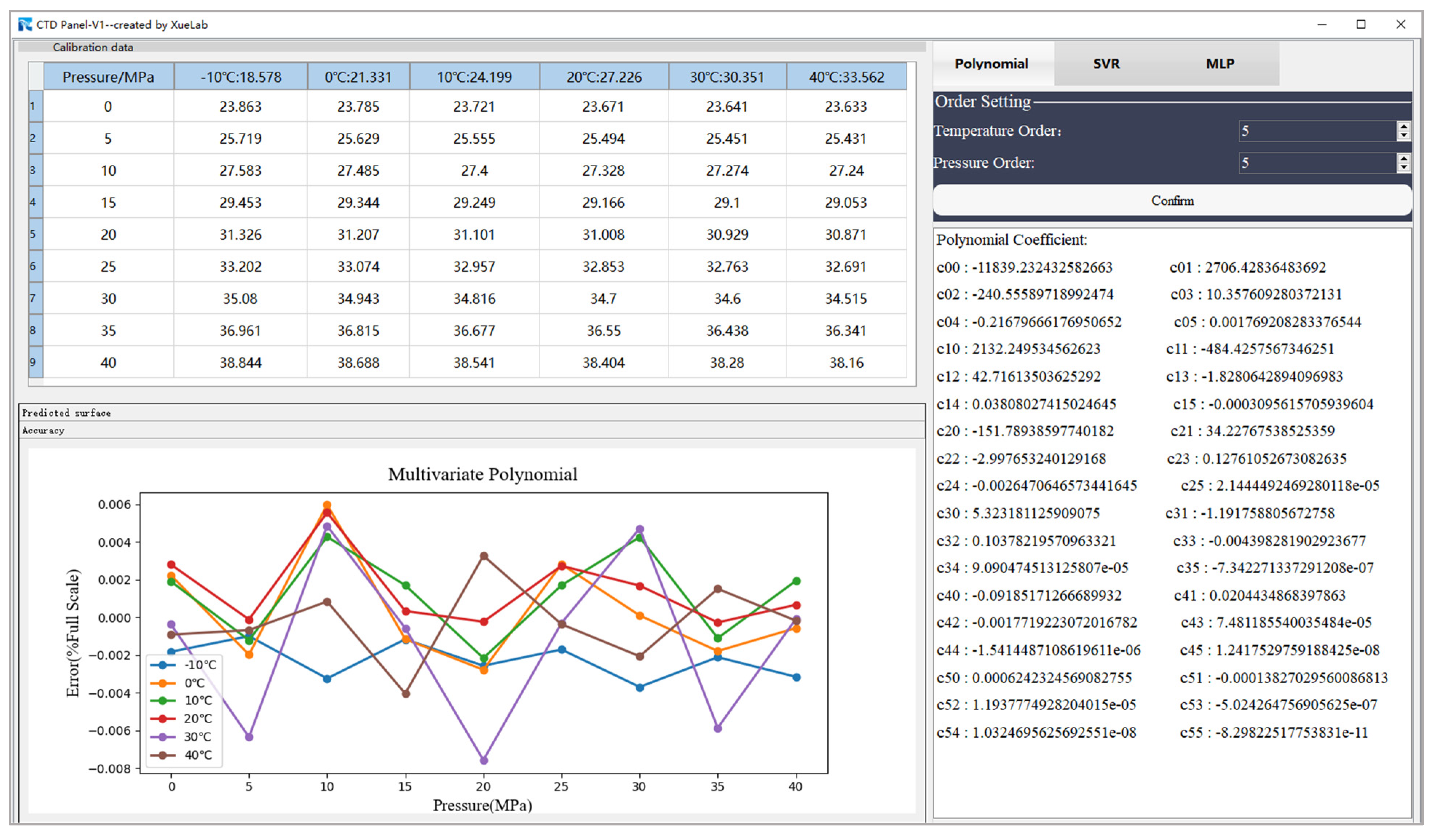
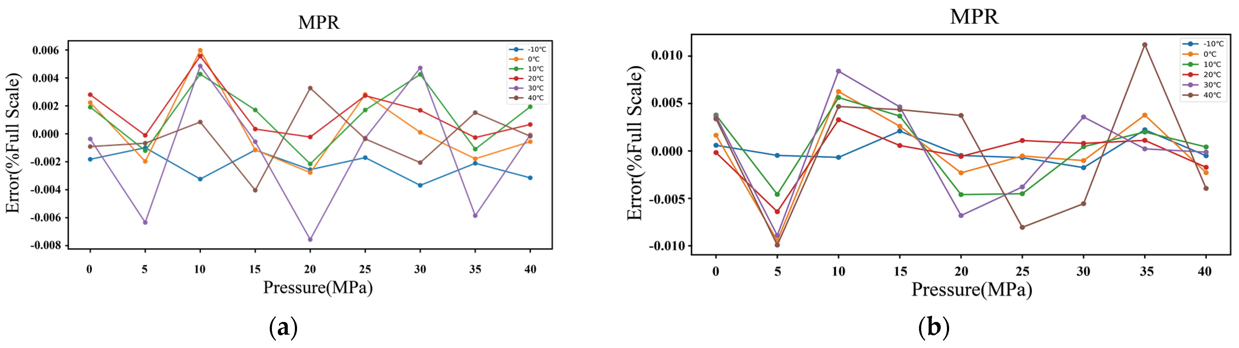
3.2. Temperature Compensation Using MPR
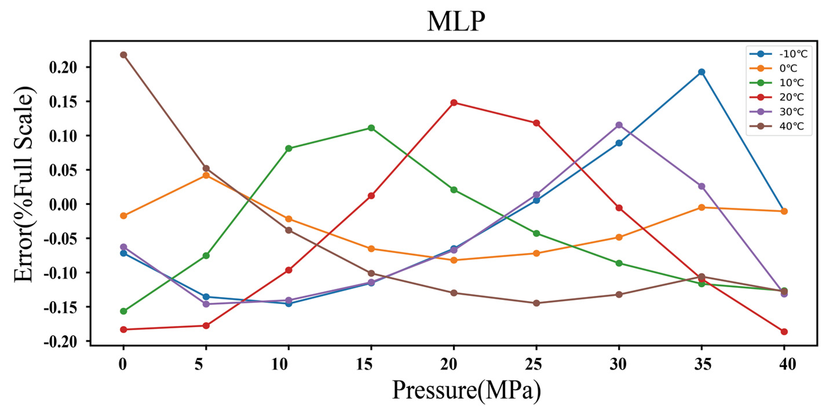
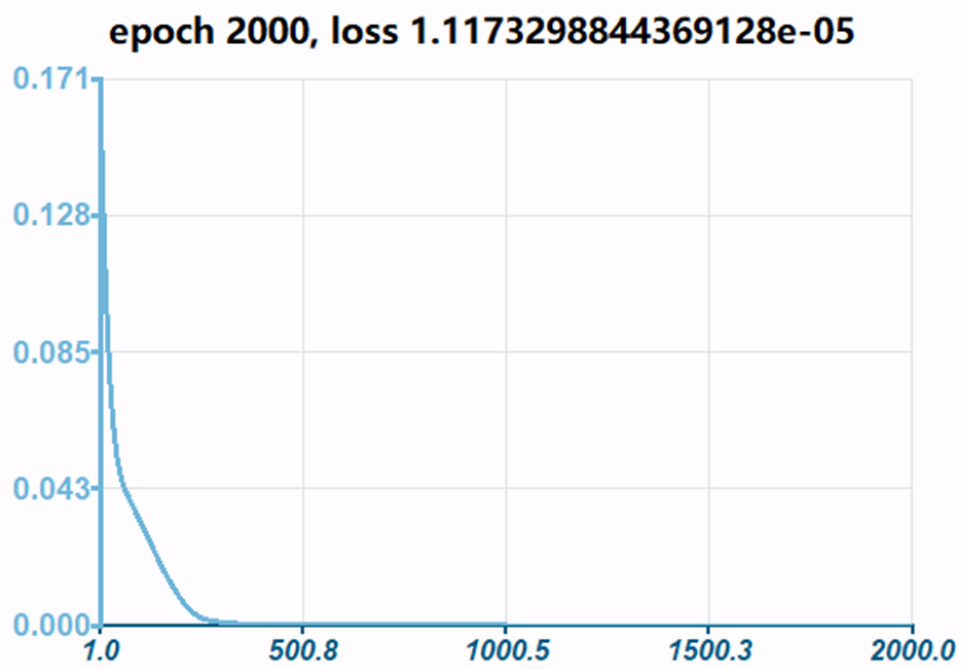
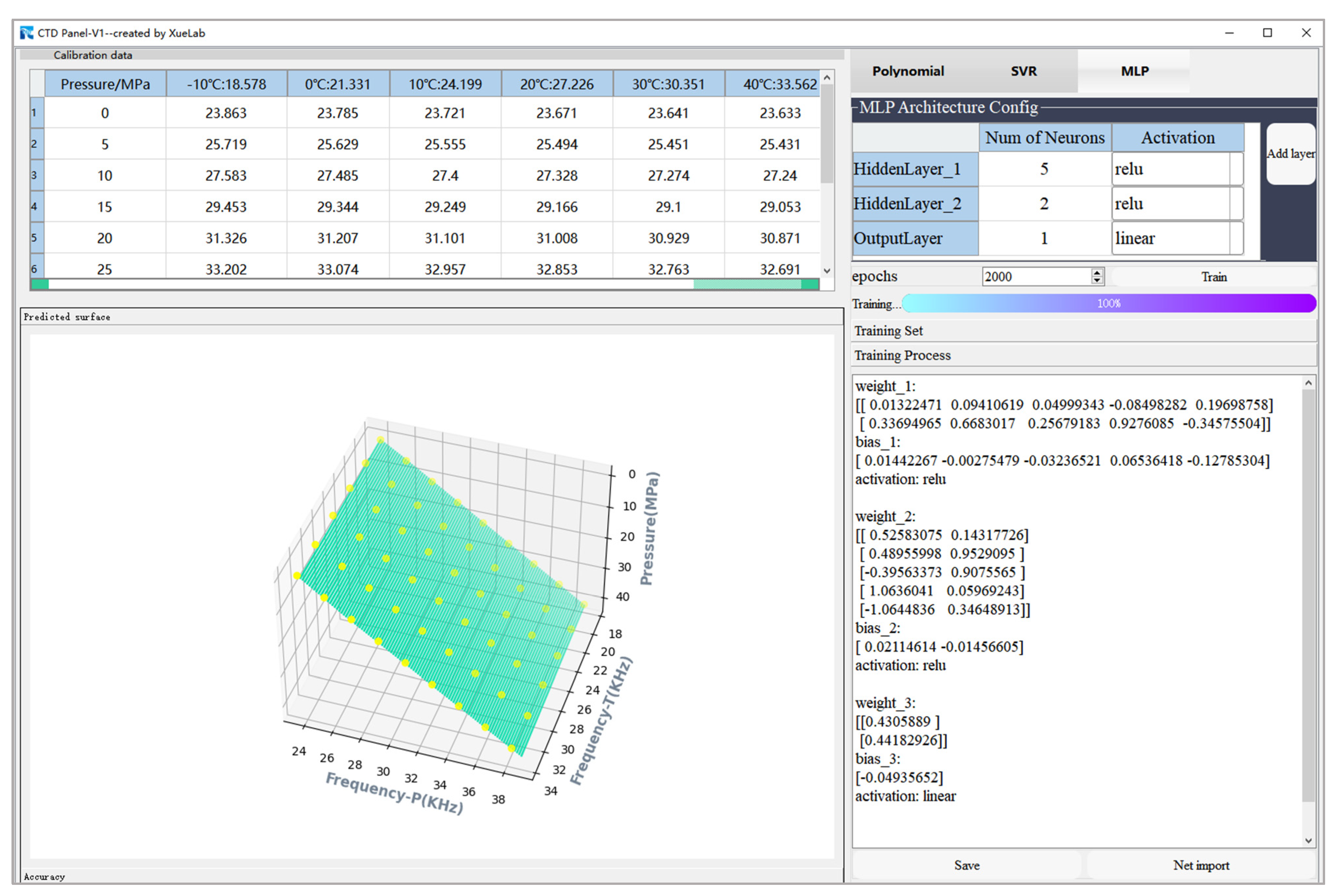
3.3. Temperature Compensation Using MLP
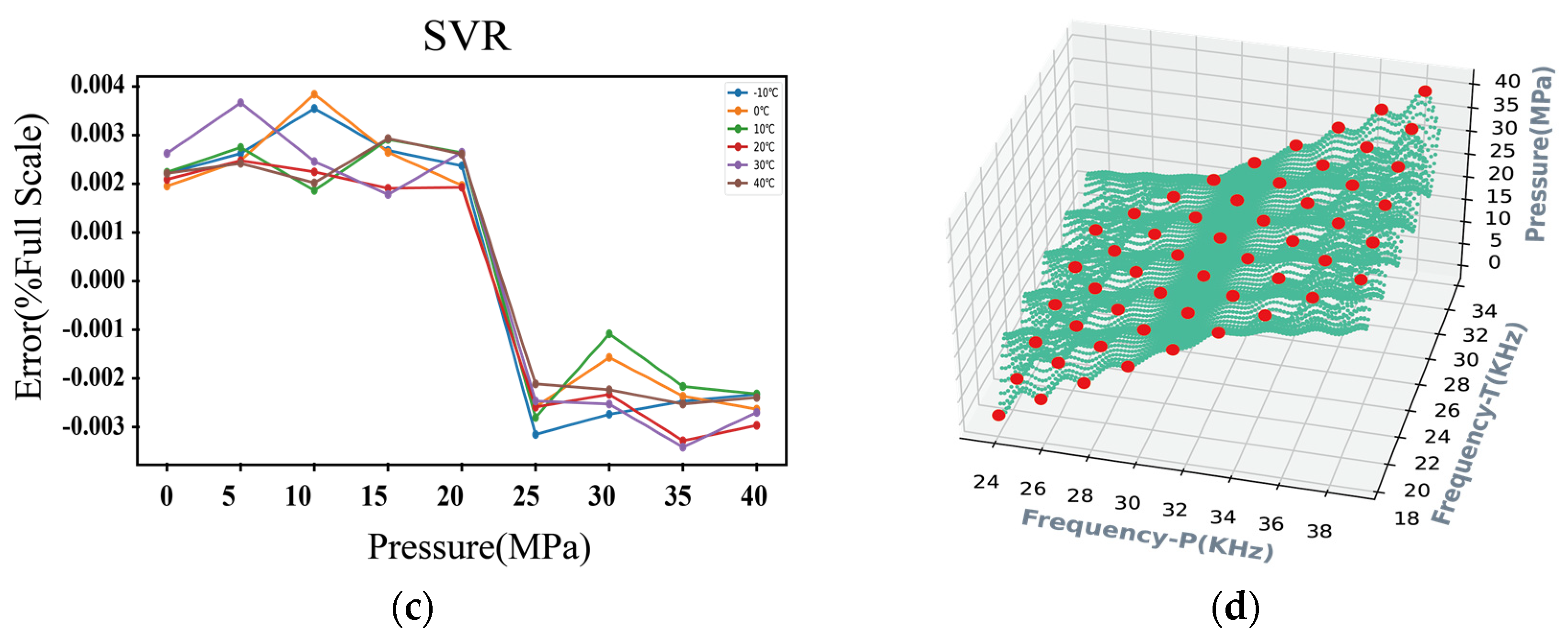
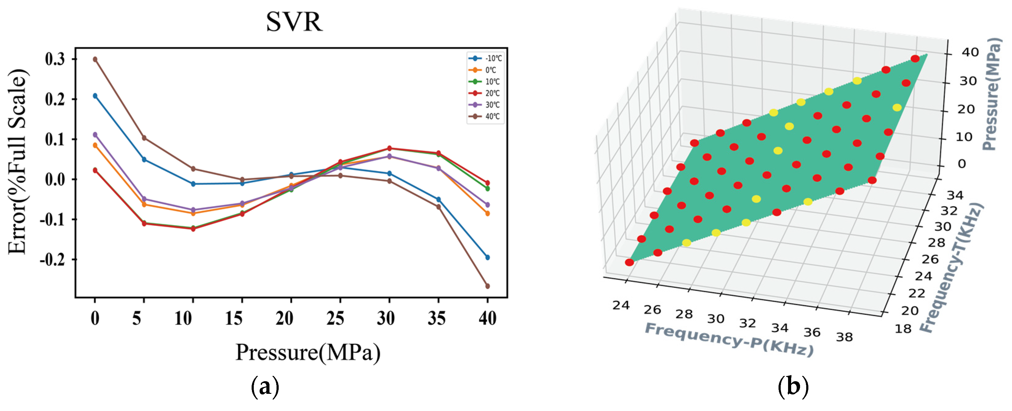
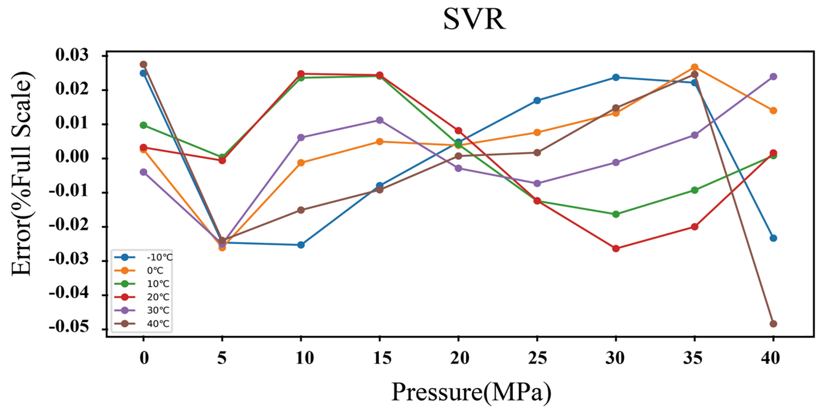
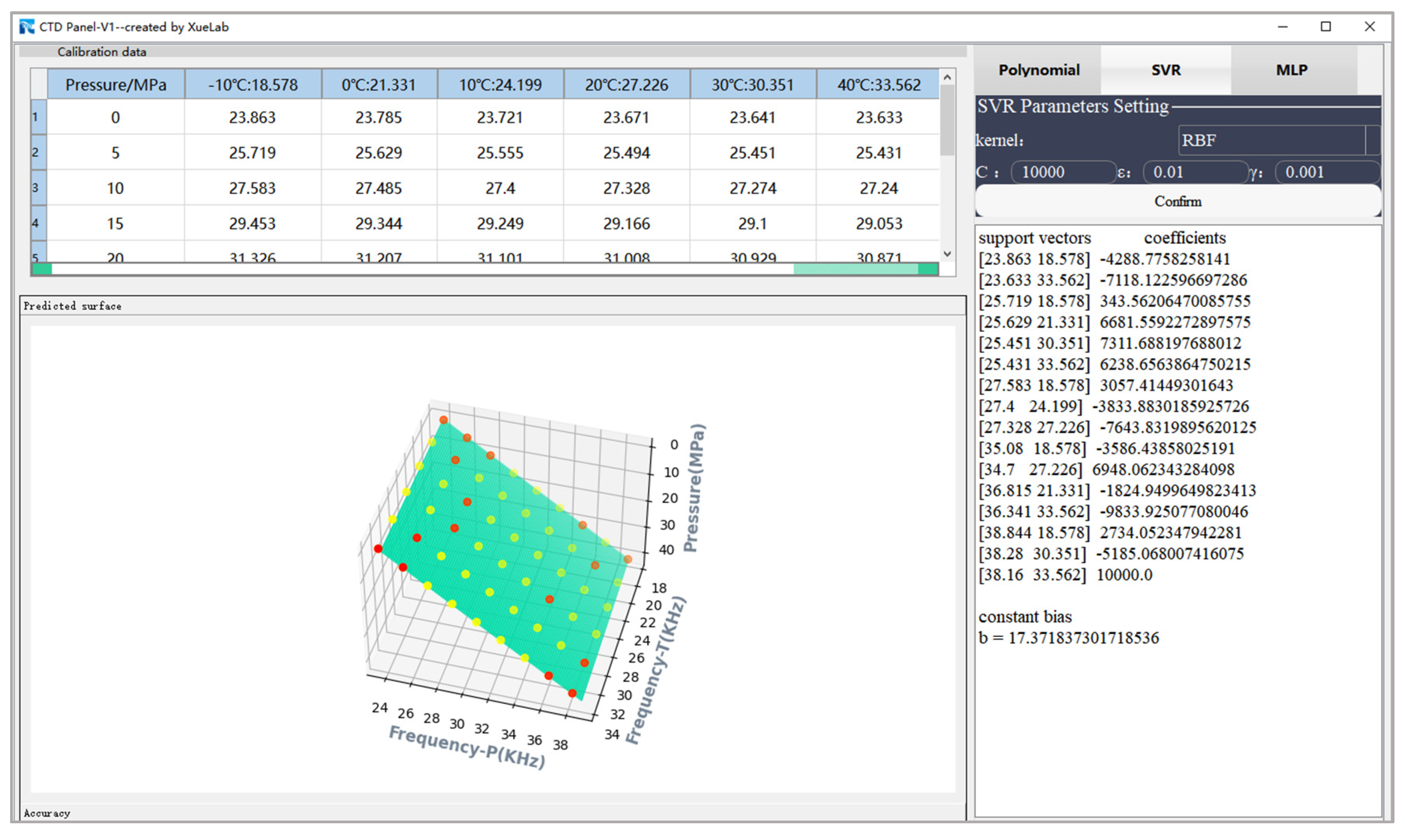
3.4. Temperature Compensation Using SVR
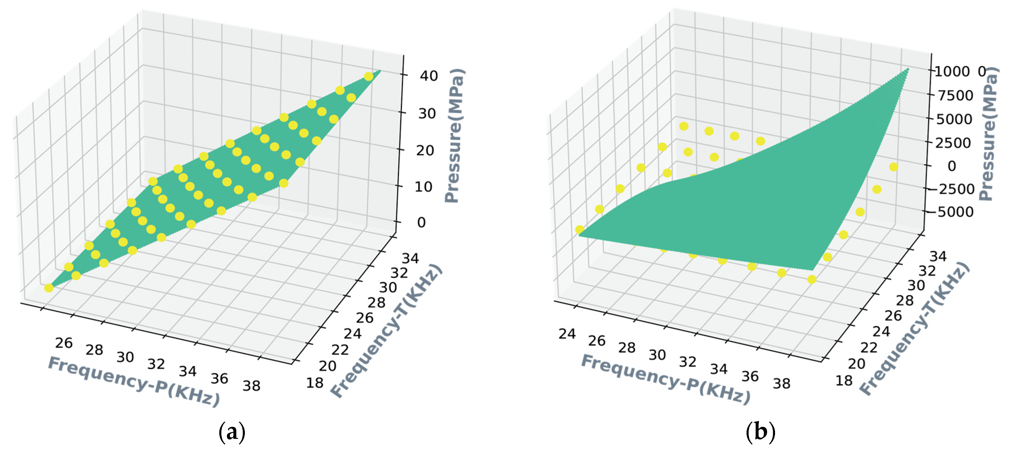
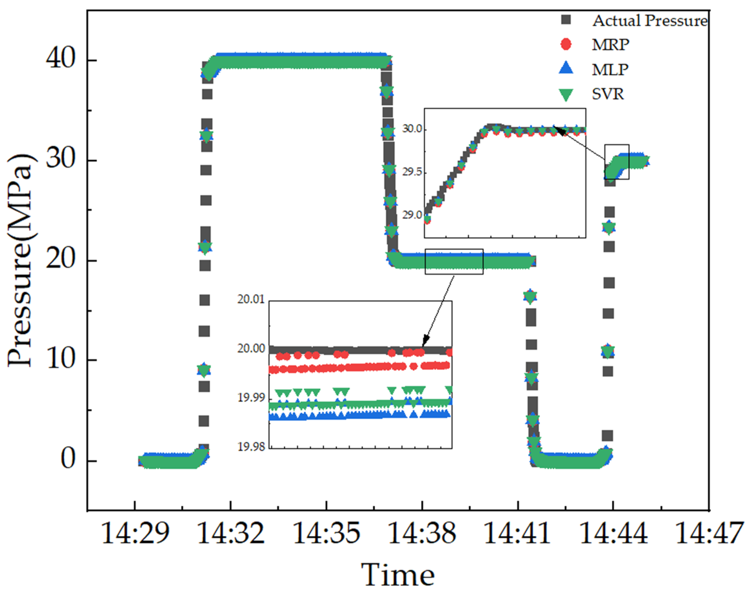
3.5. Comparison of Generalization for the Three Predominant Regression Methods
4. Discussion
5. Conclusions
Author Contributions
Funding
Data Availability Statement
Conflicts of Interest
References
- Javed, Y.; Mansoor, M.; Shah, I.A. A review of principles of MEMS pressure sensing with its aerospace applications. Sens. Rev. 2019, 39, 652–664. [Google Scholar] [CrossRef]
- Shi, Y.; Kong, D.R.; Ma, X. Research on thermal protection of piezoelectric pressure sensor for shock wave pressure measurement in explosion field. Sens. Rev. 2023, 43, 208–220. [Google Scholar] [CrossRef]
- Eernisse, E.P.; Wiggins, R. Review of thickness-shear mode quartz resonator sensors for temperature and pressure. IEEE Sens. J. 2001, 1, 79–87. [Google Scholar] [CrossRef]
- Matko, V. Next Generation AT-Cut Quartz Crystal Sensing Devices. Sensors 2011, 11, 4474–4482. [Google Scholar] [CrossRef] [PubMed]
- Sinha, B.K.; Patel, M.S. Recent developments in high precision quartz and Langasite pressure sensors for high temperature and high pressure applications. In Proceedings of the 2016 IEEE International Frequency Control Symposium (IFCS), New Orleans, LA, USA, 9–12 May 2016; pp. 1–13. [Google Scholar]
- Pham, T.T.; Zhang, H.; Yenuganti, S.; Kaluvan, S.; Kosinski, J.A. Design, Modeling, and Experiment of a Piezoelectric Pressure Sensor Based on a Thickness-Shear-Mode Crystal Resonator. IEEE Trans. Ind. Electron. 2017, 64, 8484–8491. [Google Scholar] [CrossRef]
- Zhang, L.M.; Wang, S.Y.; Xie, L.; Ma, T.; Du, J.K.; Wang, J.; Yong, Y. Frequency-Temperature Relations of Novel Cuts of Quartz Crystals for Thickness-Shear Resonators. IEEE Trans. Ind. Electron. 2017, 64, 8484–8491. [Google Scholar]
- Yu, Z.; Zhao, Y.; Li, L.; Tian, B.; Li, C. Geometry optimization for micro-pressure sensor considering dynamic interference. Rev. Sci. Instrum. 2014, 85, 095002. [Google Scholar] [CrossRef] [PubMed]
- Myers, D.R.; Azevedo, R.G.; Chen, L.; Mehregany, M.; Pisano, A.P. Passive Substrate Temperature Compensation of Doubly Anchored Double-Ended Tuning Forks. J. Microelectromech. Syst. 2012, 21, 1321–1328. [Google Scholar] [CrossRef]
- Li, Y.; Wang, J.; Luo, Z.; Chen, D.; Chen, J. A Resonant Pressure Microsensor Capable of Self-Temperature Compensation. Sensors 2015, 15, 10048–10058. [Google Scholar] [CrossRef]
- Chen, Q.; Tao, Z.; Wang, Q. Frequency-temperature compensation of piezoelectric resonators by electric DC bias field. IEEE Trans. Ultrason. Ferroelectr. Freq. Control 2005, 52, 1627–1631. [Google Scholar] [CrossRef]
- Santos, E.J.P.; Silva, L.B.; Technology, P. High-resolution pressure transducer design and associated circuitry to build a network-ready smart sensor for distributed measurement in oil and gas production wells. J. Pet. Explor. Prod. Technol. 2022, 12, 2083–2092. [Google Scholar] [CrossRef]
- Xiang, C.; Lu, Y.; Yan, P.; Chen, J.; Wang, J.; Chen, D. A Resonant Pressure Microsensor with Temperature Compensation Method Based on Differential Outputs and a Temperature Sensor. Micromachines 2020, 11, 1022. [Google Scholar] [CrossRef]
- Kazemi, N.; Abdolrazzaghi, M.; Musílek, P. Comparative Analysis of Machine Learning Techniques for Temperature Compensation in Microwave Sensors. IEEE Trans. Microw. Theory Tech. 2021, 69, 4223–4236. [Google Scholar] [CrossRef]
- Mao, Z.; Peng, Y.; Hu, C.; Ding, R.; Yamada, Y.; Maeda, S. Soft computing-based predictive modeling of flexible electrohydrodynamic pumps. Biomim. Intell. Robot. 2023, 3, 100114. [Google Scholar] [CrossRef]
- Montesinos López, O.A.; Montesinos López, A.; Crossa, J. Multivariate Statistical Machine Learning Methods for Genomic Prediction; Springer International Publishing: Cham, Switzerland, 2022. [Google Scholar]
- Izonin, I.; Tkachenko, R.; Greguš, M.; Zub, K.; Lotoshynska, N. Input Doubling Method based on SVR with RBF kernel in Clinical Practice: Focus on Small Data. Procedia Comput. Sci. 2021, 184, 606–613. [Google Scholar] [CrossRef]
- Clayton, L.D.; Eernisse, E.P. Quartz thickness-shear mode pressure sensor design for enhanced sensitivity. IEEE Trans. Ultrason. Ferroelectr. Freq. Control. 1998, 45, 1196–1203. [Google Scholar] [CrossRef]
- Erhart, J.; Rusin, L.Y.; Seifert, L. Resonant frequency temperature coefficients for the piezoelectric resonators working in various vibration modes. J. Electroceramics 2007, 19, 403–406. [Google Scholar] [CrossRef]
- Silva, L.B.M.; Santos, E. Modeling high-resolution down-hole pressure transducer to achieve semi-distributed measurement in oil and gas production wells. J. Integr. Circuits Syst. 2019, 14, 9. [Google Scholar] [CrossRef]
- Besson, R.J.; Boy, J.J.; Glotin, B.J.P.; Jinzaki, Y.; Sinha, B.K.; Valdois, M. A dual-mode thickness-shear quartz pressure sensor. IEEE Trans. Ultrason. Ferroelectr. Freq. Control. 1993, 40, 584–591. [Google Scholar] [CrossRef]
- Patel, M.S.; Sinha, B.K. Influence of Viscoelastic Stress Relaxation of Glass-Frit Sealing Layer on the Frequency Stability of a Dual-Mode Quartz Pressure Sensor Under Extreme Pressure Conditions. In Proceedings of the 2018 IEEE International Ultrasonics Symposium (IUS), Kobe, Japan, 22–25 October 2018; pp. 1–4. [Google Scholar]
- Chkifa, A.; Cohen, A.; Migliorati, G.; Nobile, F.; Tempone, R. Discrete least squares polynomial approximation with random evaluations—Application to parametric and stochastic elliptic PDEs. ESAIM Math. Model. Numer. Anal. 2015, 49, 815–837. [Google Scholar] [CrossRef]
- Migliorati, G.; Nobile, F. Analysis of discrete least squares on multivariate polynomial spaces with evaluations at low-discrepancy point sets. J. Complex. 2015, 31, 517–542. [Google Scholar] [CrossRef]
- Boor, C.d.; Ron, A. Computational aspects of polynomial interpolation in several variables. Math. Comput. 1992, 58, 705–727. [Google Scholar] [CrossRef]
- Binev, P.; Cohen, A.; Dahmen, W.; DeVore, R. Universal Algorithms for Learning Theory. Part II: Piecewise Polynomial Functions. Constr. Approx. 2007, 26, 127–152. [Google Scholar] [CrossRef]
- Castro, Y.d.; Gamboa, F.; Henrion, D.; Hess, R.; Lasserre, J.B. Approximate Optimal Designs for Multivariate Polynomial Regression. Ann. Stat. 2019, 47, 127–155. [Google Scholar] [CrossRef]
- Alzubaidi, L.; Zhang, J.; Humaidi, A.J.; Al-dujaili, A.; Duan, Y.; Al-Shamma, O.; Santamaría, J.I.; Fadhel, M.A.; Al-Amidie, M.; Farhan, L. Review of deep learning: Concepts, CNN architectures, challenges, applications, future directions. J. Big Data 2021, 8, 1–74. [Google Scholar] [CrossRef]
- Ballard, Z.S.; Joung, H.-A.; Goncharov, A.; Liang, J.; Nugroho, K.; Di Carlo, D.; Garner, O.B.; Ozcan, A. Deep learning-enabled point-of-care sensing using multiplexed paper-based sensors. NPJ Digit. Med. 2020, 3, 1–8. [Google Scholar] [CrossRef]
- Tolstikhin, I.O.; Houlsby, N.; Kolesnikov, A.; Beyer, L.; Zhai, X.; Unterthiner, T.; Yung, J.; Keysers, D.; Uszkoreit, J.; Lucic, M.; et al. MLP-Mixer: An all-MLP Architecture for Vision. In Proceedings of the Neural Information Processing Systems, Virtual, 6–14 December 2021. [Google Scholar]
- Ceriotti, M. Beyond potentials: Integrated machine learning models for materials. MRS Bull. 2022, 47, 1045–1053. [Google Scholar] [CrossRef]
- Huang, J.; Zhang, J.; Li, X.; Qiao, Y.; Zhang, R.; Kumar, G.S. Investigating the effects of ensemble and weight optimization approaches on neural networks’ performance to estimate the dynamic modulus of asphalt concrete. Road Mater. Pavement Des. 2022, 24, 1939–1959. [Google Scholar] [CrossRef]
- Wen, H.; Xie, W.; Pei, J. A pre-radical basis function with deep back propagation neural network research. In Proceedings of the 2014 12th International Conference on Signal Processing (ICSP), Hangzhou, China, 19–23 October 2014; pp. 1489–1494. [Google Scholar]
- Zhang, F.; O’Donnell, L. Support Vector Regression. In Machine Learning, 1st ed.; Andrea, M., Sandra, V., Eds.; Academic Press: London, UK, 2020; pp. 123–140. [Google Scholar]
- Drucker, H.; Burges, C.J.C.; Kaufman, L.; Smola, A.; Vapnik, V.N. Support Vector Regression Machines. In Proceedings of the Neural Information Processing Systems, Denver, CO, USA, 2–5 December 1996. [Google Scholar]
- Li, H.-D.; Liang, Y.; Xu, Q.J.C.; Systems, I.L. Support vector machines and its applications in chemistry. Chemom. Intell. Lab. Syst. 2009, 95, 188–198. [Google Scholar] [CrossRef]
- Huang, G.-B.; Zhou, H.; Ding, X.; Zhang, R. Extreme Learning Machine for Regression and Multiclass Classification. IEEE Trans. Syst. Man Cybern. Part B Cybern. 2012, 42, 513–529. [Google Scholar] [CrossRef] [PubMed]
- Chang, C.-C.; Lin, C.-J. LIBSVM: A library for support vector machines. ACM Trans. Intell. Syst. Technol. 2011, 2, 21–27. [Google Scholar] [CrossRef]
- Canatar, A.; Bordelon, B.; Pehlevan, C. Spectral bias and task-model alignment explain generalization in kernel regression and infinitely wide neural networks. Nat. Commun. 2021, 12, 2914. [Google Scholar] [CrossRef] [PubMed]
- Nhu, V.-H.; Hoang, N.-D.; Nguyen, H.; Ngo, P.-T.T.; Thanh Bui, T.; Hoa, P.V.; Samui, P.; Tien Bui, D. Effectiveness assessment of Keras based deep learning with different robust optimization algorithms for shallow landslide susceptibility mapping at tropical area. CATENA 2020, 188, 104458. [Google Scholar] [CrossRef]
- Ali, I.; Asif, M.; Shehzad, K.; Rehman, M.R.u.; Kim, D.G.; Rikan, B.S.; Pu, Y.; Yoo, S.-S.; Lee, K. A Highly Accurate, Polynomial-Based Digital Temperature Compensation for Piezoresistive Pressure Sensor in 180 nm CMOS Technology. Sensors 2020, 20, 5256. [Google Scholar] [CrossRef]
- Hsia, J.-Y.; Lin, C.-J. Parameter Selection for Linear Support Vector Regression. IEEE Trans. Neural Netw. Learn. Syst. 2020, 31, 5639–5644. [Google Scholar] [CrossRef]


| Method | Maximum Absolute Error (MPa) | The Residual Error at all Temperatures of Full Scale | Rank of Generalization Ability |
|---|---|---|---|
| MPR | 0.0032 | 0.008% FS | High |
| MLP | 0.12 | 0.3% FS | Low |
| SVR | 0.02 | 0.05% FS | Middle |
Disclaimer/Publisher’s Note: The statements, opinions and data contained in all publications are solely those of the individual author(s) and contributor(s) and not of MDPI and/or the editor(s). MDPI and/or the editor(s) disclaim responsibility for any injury to people or property resulting from any ideas, methods, instructions or products referred to in the content. |
© 2023 by the authors. Licensee MDPI, Basel, Switzerland. This article is an open access article distributed under the terms and conditions of the Creative Commons Attribution (CC BY) license (https://creativecommons.org/licenses/by/4.0/).
Share and Cite
Yao, B.; Xu, Y.; Jing, J.; Zhang, W.; Guo, Y.; Zhang, Z.; Zhang, S.; Liu, J.; Xue, C. Comparison and Verification of Three Algorithms for Accuracy Improvement of Quartz Resonant Pressure Sensors. Micromachines 2024, 15, 23. https://doi.org/10.3390/mi15010023
Yao B, Xu Y, Jing J, Zhang W, Guo Y, Zhang Z, Zhang S, Liu J, Xue C. Comparison and Verification of Three Algorithms for Accuracy Improvement of Quartz Resonant Pressure Sensors. Micromachines. 2024; 15(1):23. https://doi.org/10.3390/mi15010023
Chicago/Turabian StyleYao, Bin, Yanbo Xu, Junming Jing, Wenjun Zhang, Yuzhen Guo, Zengxing Zhang, Shiqiang Zhang, Jianwei Liu, and Chenyang Xue. 2024. "Comparison and Verification of Three Algorithms for Accuracy Improvement of Quartz Resonant Pressure Sensors" Micromachines 15, no. 1: 23. https://doi.org/10.3390/mi15010023
APA StyleYao, B., Xu, Y., Jing, J., Zhang, W., Guo, Y., Zhang, Z., Zhang, S., Liu, J., & Xue, C. (2024). Comparison and Verification of Three Algorithms for Accuracy Improvement of Quartz Resonant Pressure Sensors. Micromachines, 15(1), 23. https://doi.org/10.3390/mi15010023