
Microrobot Path Planning Based on the Multi-Module DWA Method in Crossing Dense Obstacle Scenario


 ,
,
Abstract
1. Introduction
1.1. Literature Review
1.2. Our Contributions
- By combining the Mahalanobis distance, Frobenius norm, and covariance matrix, a method for judging obstacle-dense areas has been proposed for the first time. The method can locate these areas roughly and help avoid obstacles by estimating the distribution of obstacles overall. This method has the foresight to ensure the safety of robot operation;
- To improve the ability of the robot to navigate to target points, the original evaluation function of DWA is modified and a new evaluation function based on target points is added;
- This paper combines EDWA with a two-dimensional analytic vector field method with a good obstacle avoidance effect to produce a multi-module hybrid algorithm to detect the location of obstacle-dense areas in real time and change the planning strategy. DWA’s poor obstacle avoidance effect in dense areas is addressed by this paper by combining EDWA with this method;
- An improved immune algorithm is created to get the best weight solution based on the algorithm’s convergence iteration and to realize the dynamic change of weight combinations, improving the logicalness of path planning.
2. Basic Theory Algorithm
2.1. Principle of Traditional DWA Algorithm
2.2. Principle of Immune Algorithm
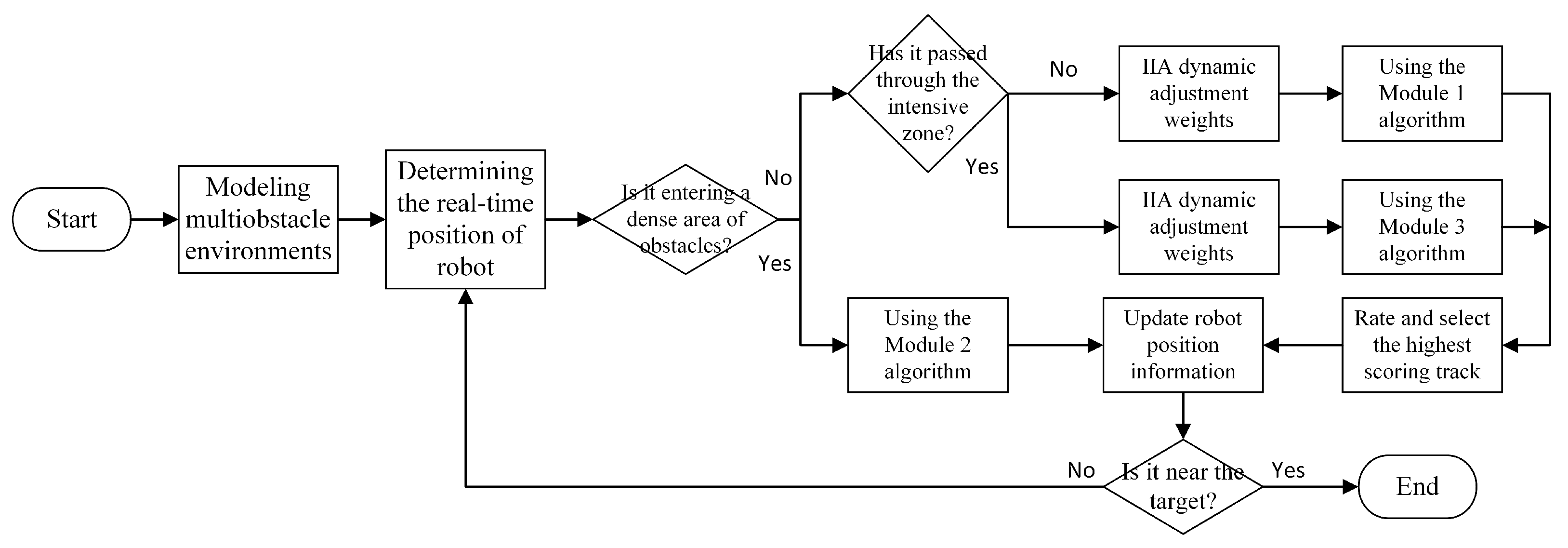
3. MEDWA-Based Planning Approach
3.1. Judgment Method of Dense Obstacle Area
3.1.1. Definition of Dense Obstacle Areas
3.1.2. Critical Moments in Dense Obstacle Areas
3.2. MEDWA Algorithm
3.2.1. EDWA Algorithm
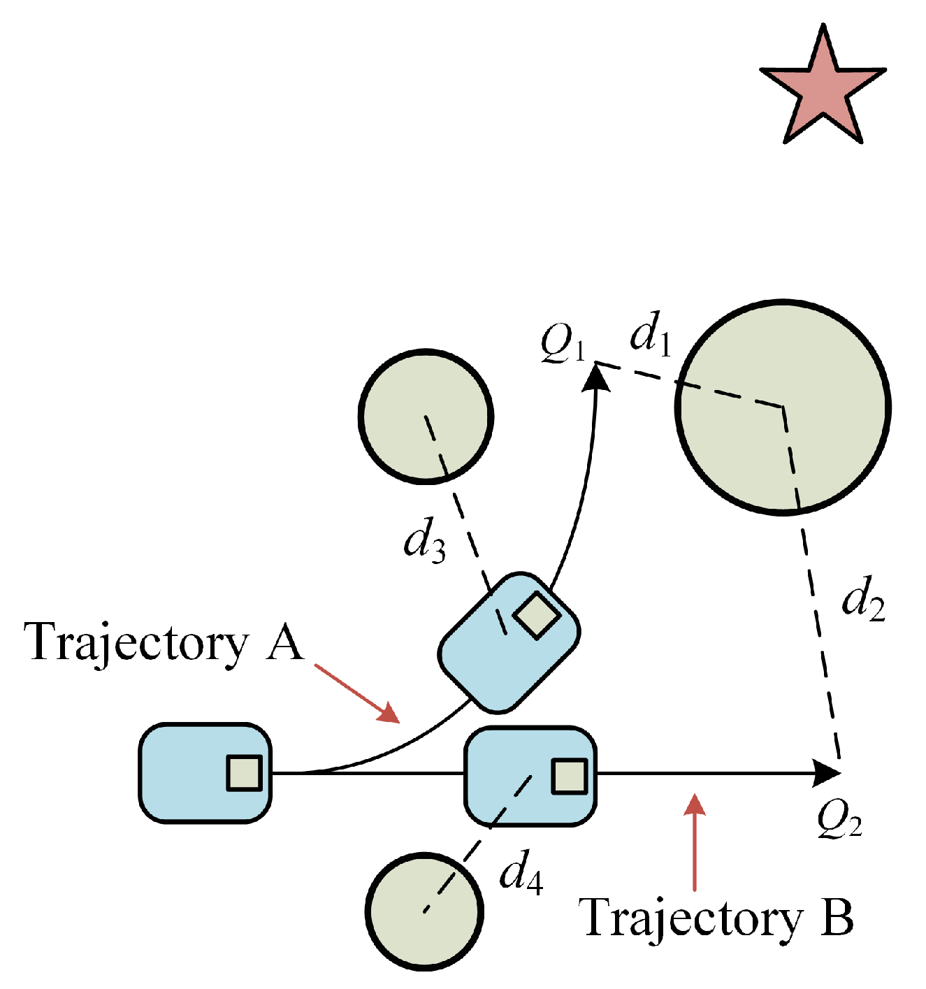
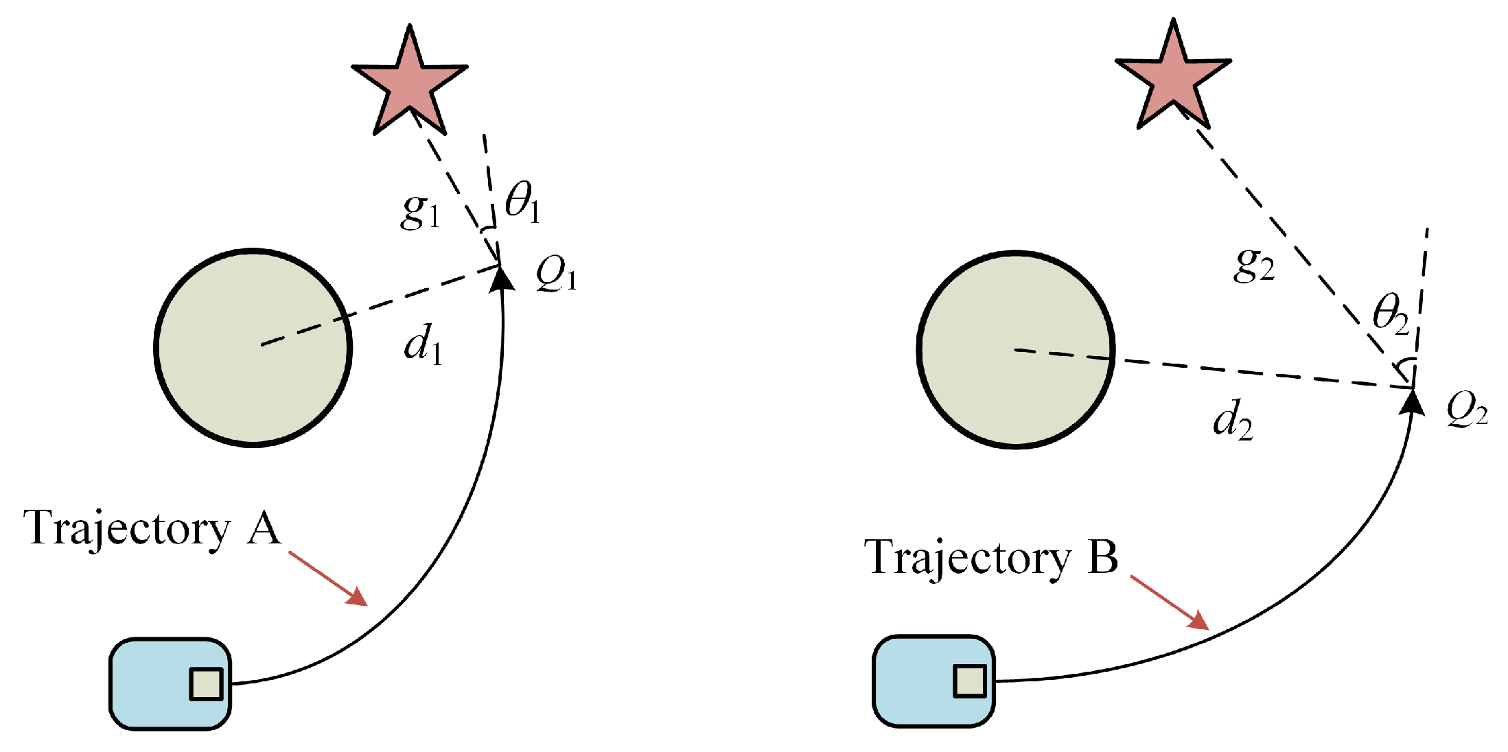
Optimized Heading Angle Function
Optimized Obstacle Function
Added Target Point Function
3.2.2. IIA Algorithm
Differential Evolution Operator
Improved Cloning Operator
4. Simulation Validation
4.1. Simulation Settings
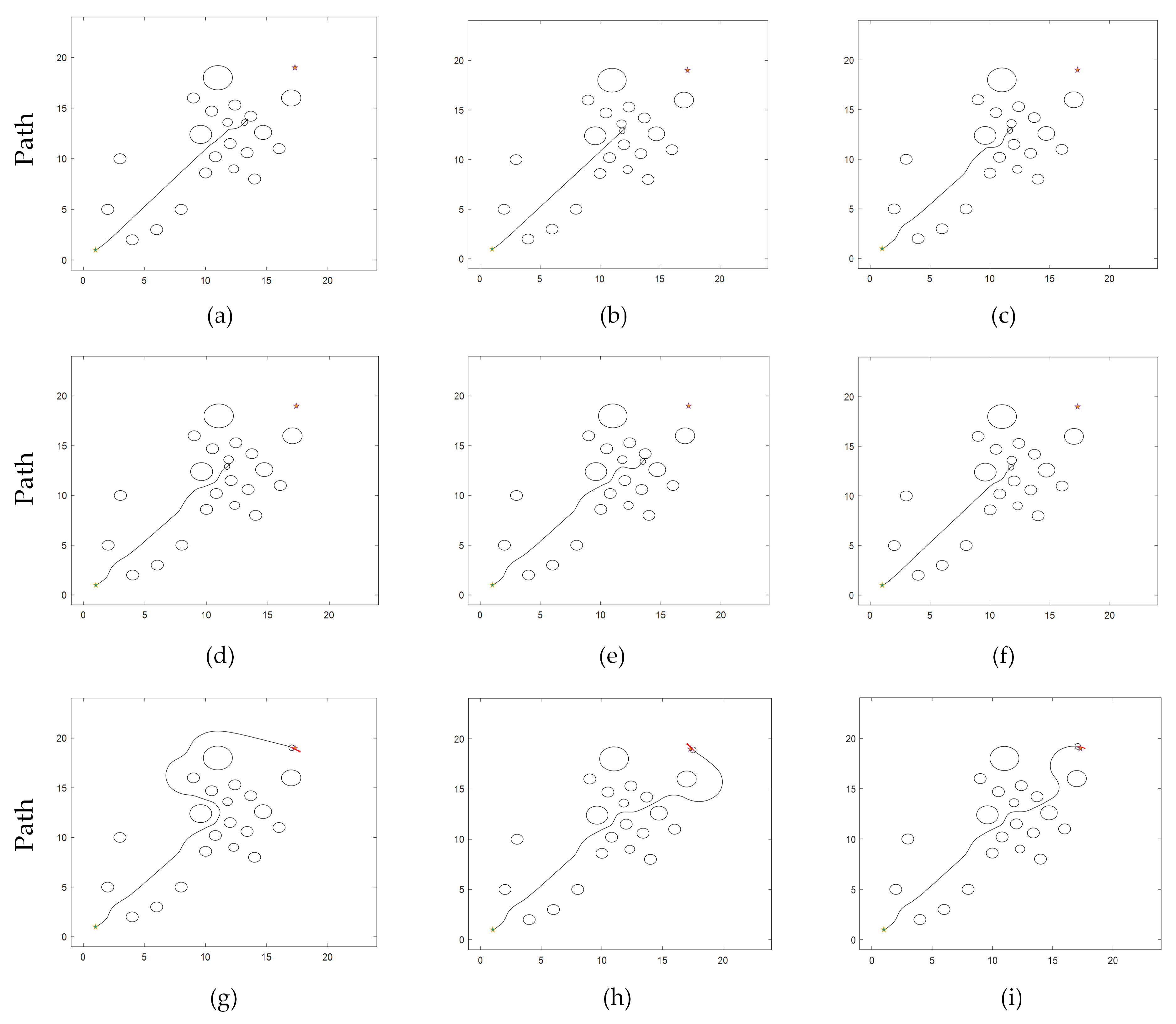
4.2. Scenario 1
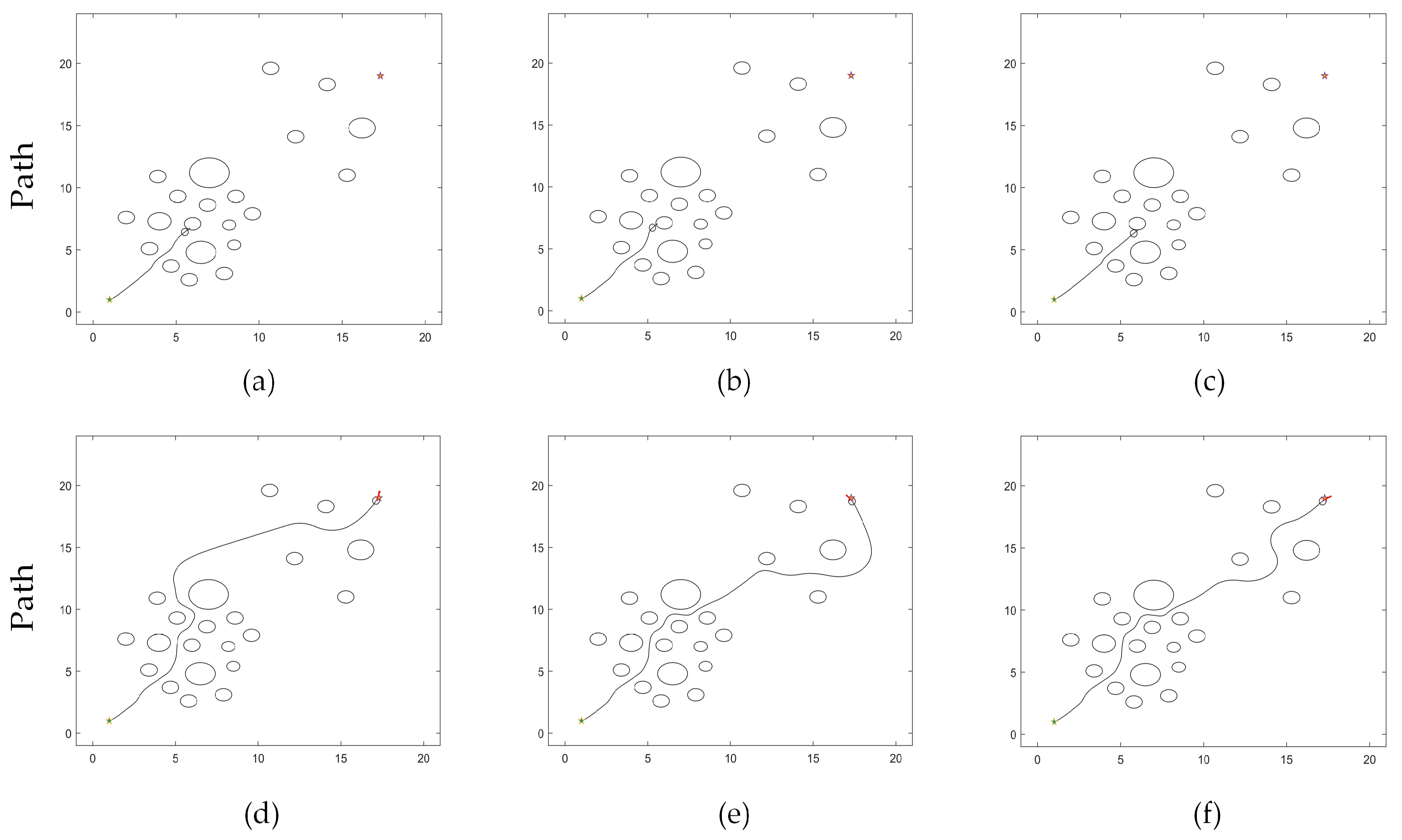
4.2.1. Simulation Results
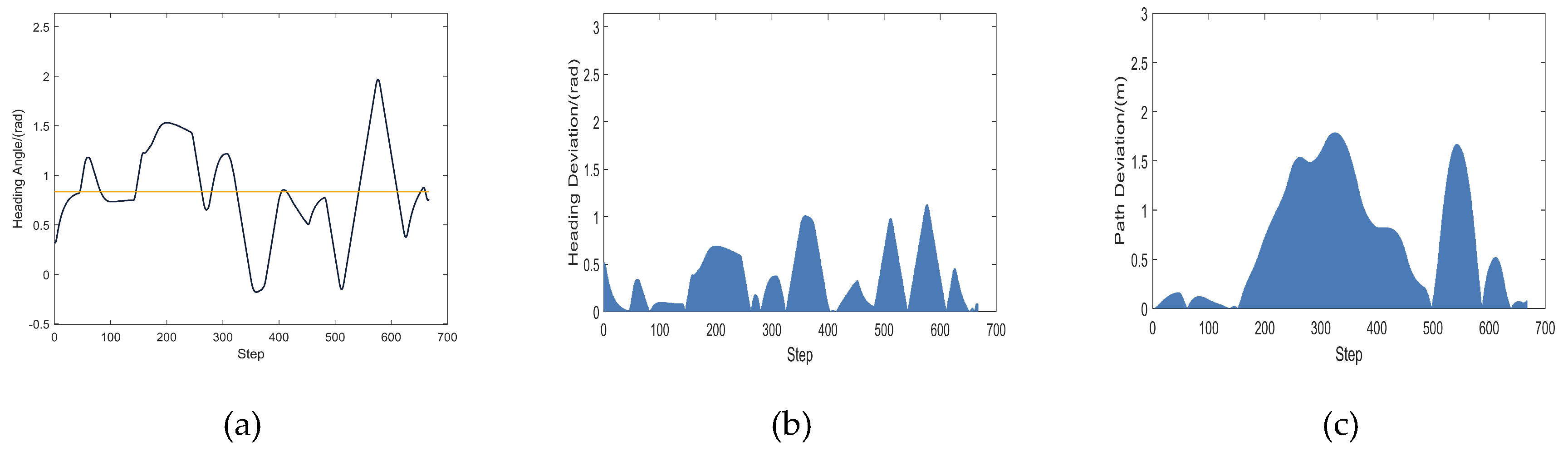
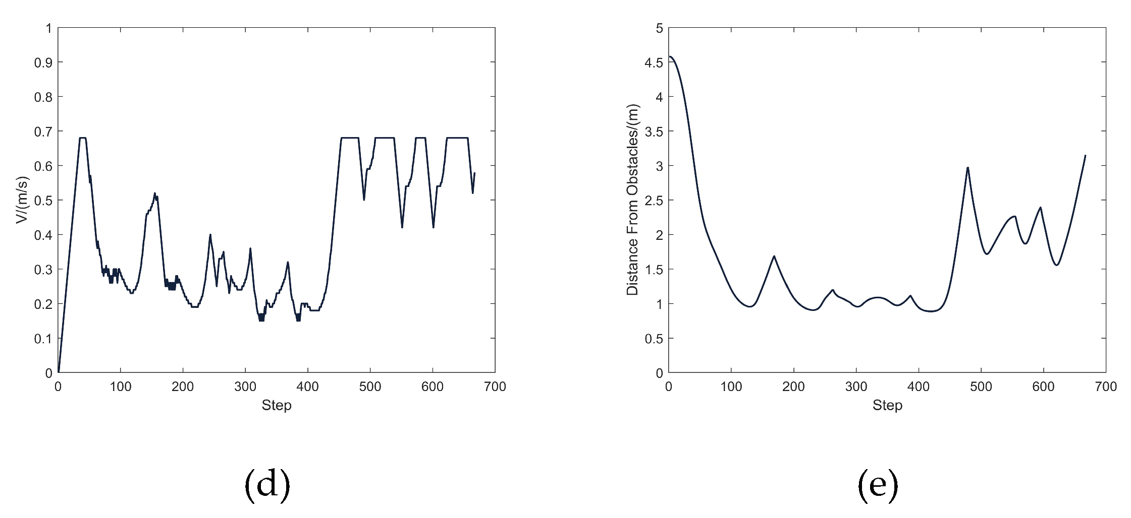
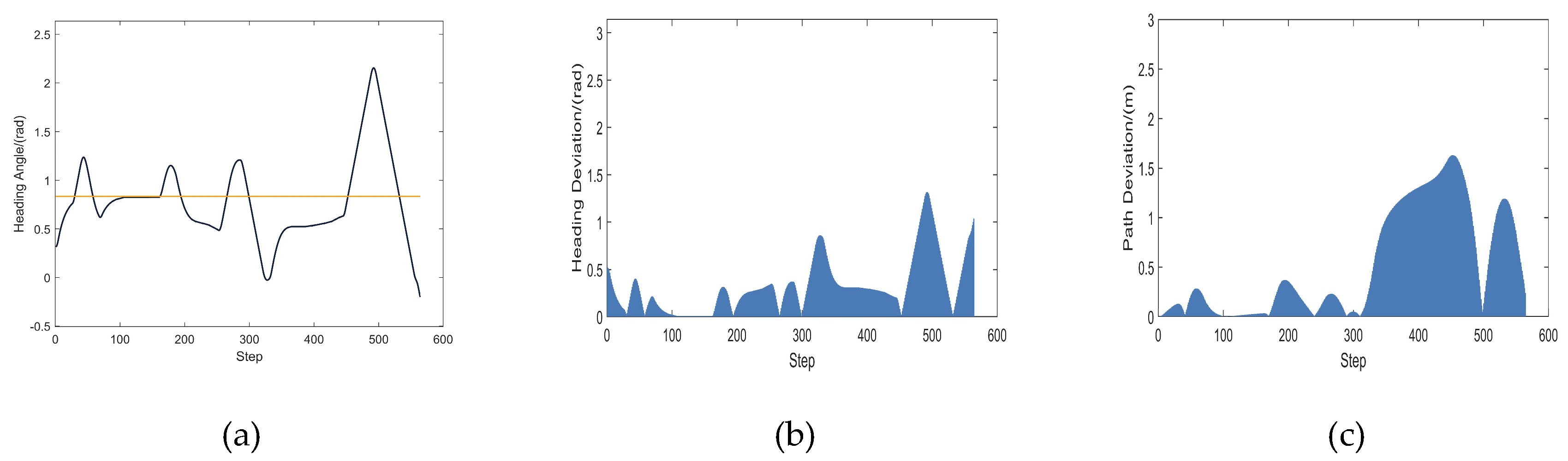
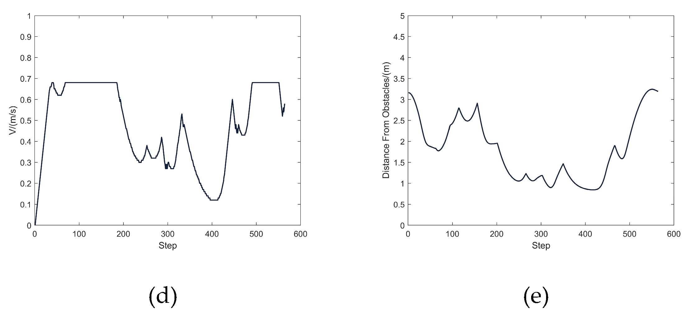
TDWA Results
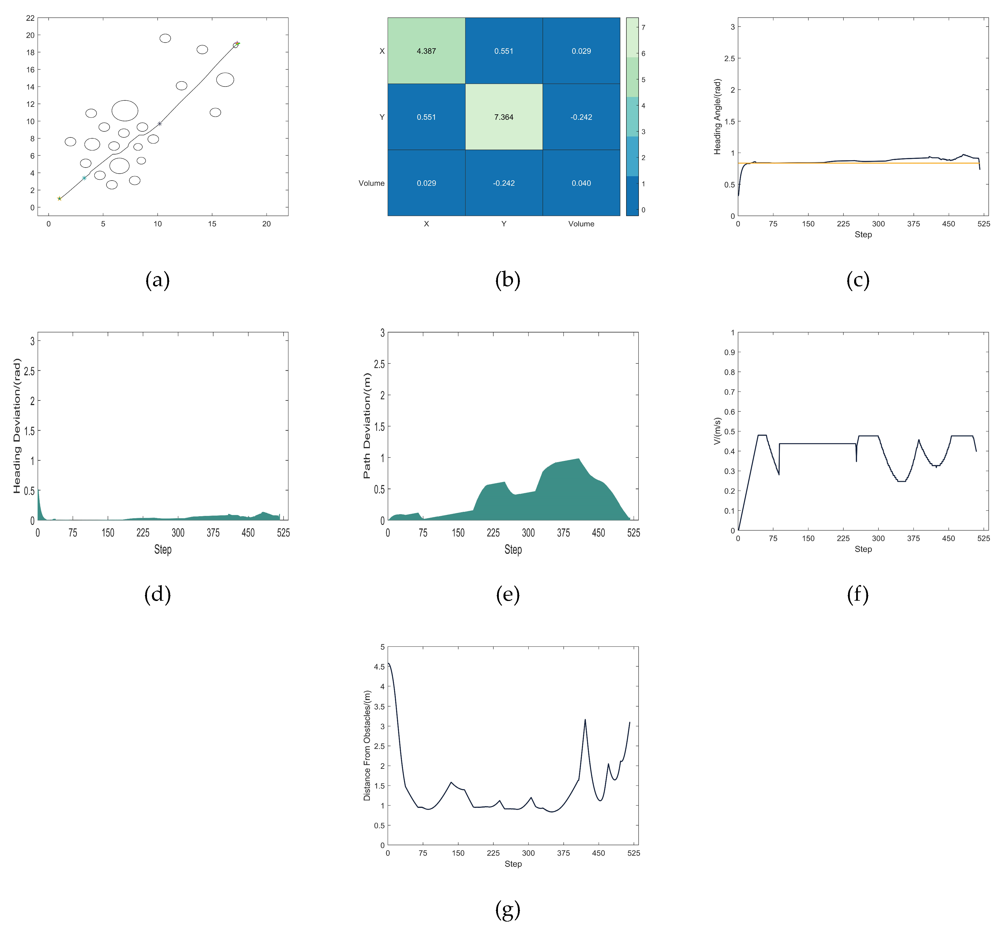
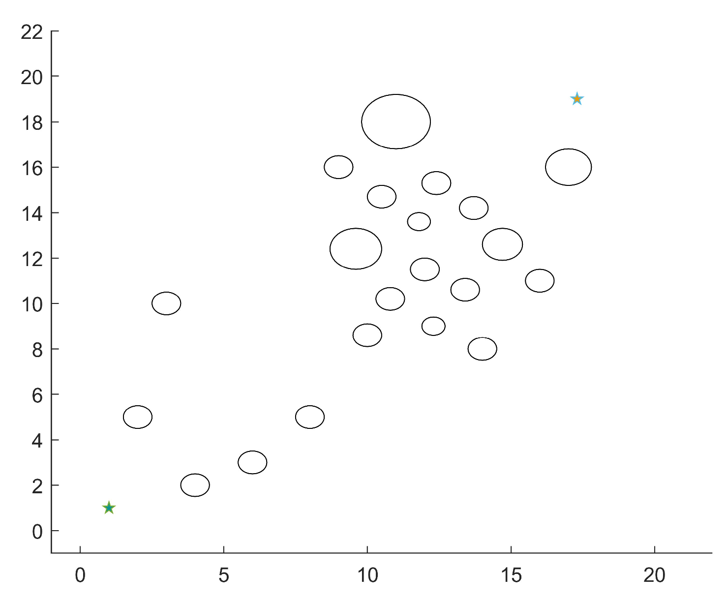
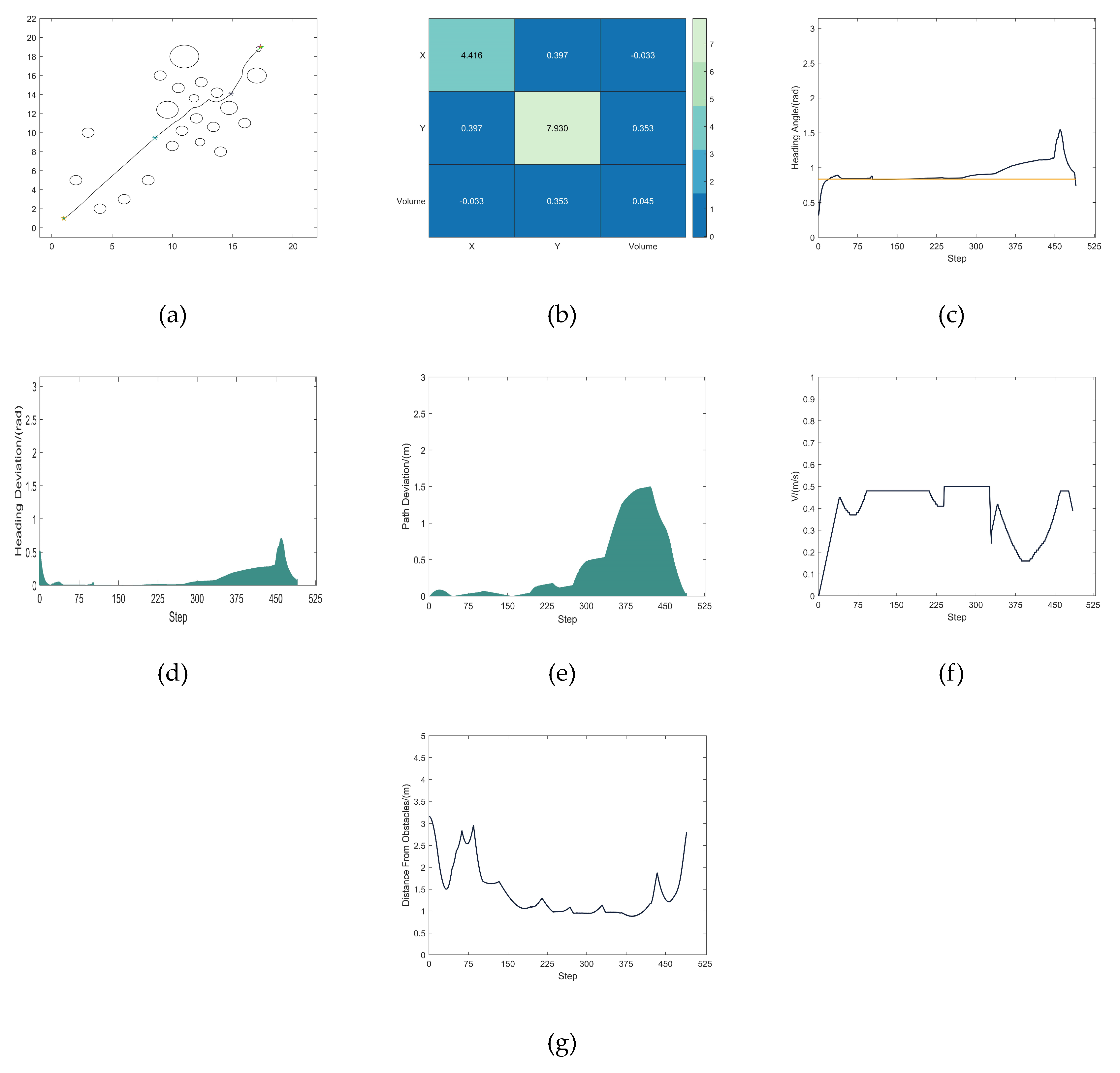
MEDWA Results
4.2.2. Analysis of Results
4.3. Scenario 2
4.3.1. Simulation Results
TDWA Results
MEDWA Results
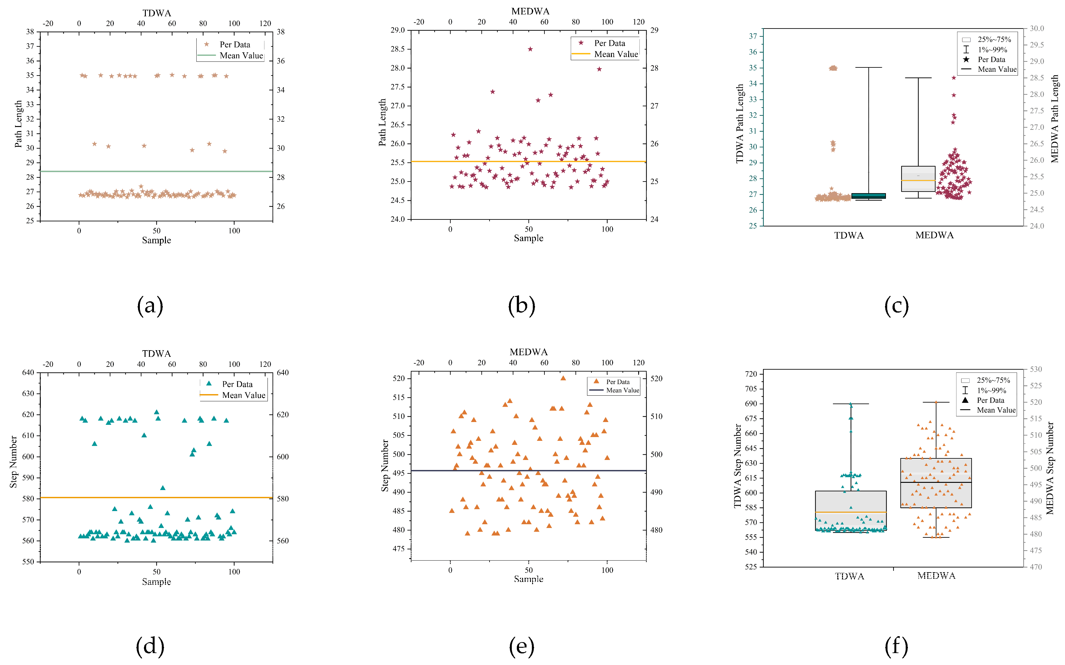
4.3.2. Analysis of Results
5. Conclusions
Author Contributions
Funding
Institutional Review Board Statement
Informed Consent Statement
Data Availability Statement
Acknowledgments
Conflicts of Interest
References
- Huang, C.; Hsu, S. Efficient Path Planning for a Microrobot Passing through Environments with Narrow Passages. Micromachines 2022, 13, 1935. [Google Scholar] [CrossRef] [PubMed]
- Guney, M.; Raptis, I. Dynamic prioritized motion coordination of multi-AGV systems. Robot. Auton. Syst. 2020, 139, 103534. [Google Scholar] [CrossRef]
- Liu, C.; Liu, A.; Wang, R.; Zhao, H.; Lu, Z. Path Planning Algorithm for Multi-Locomotion Robot Based on Multi-Objective Genetic Algorithm with Elitist Strategy. Micromachines 2022, 13, 616. [Google Scholar] [CrossRef] [PubMed]
- Wu, B.; Chi, X.; Zhao, C.; Zhang, W.; Lu, Y.; Jiang, D. Dynamic Path Planning for Forklift AGV Based on Smoothing A* and Improved DWA Hybrid Algorithm. Sensors 2022, 22, 7079. [Google Scholar] [CrossRef] [PubMed]
- Guzzi, J.; Chavez-Garcia, R.; Nava, M.; Gambardella, L.; Giusti, A. Path Planning with Local Motion Estimations. IEEE Robot. Autom. Lett. 2020, 5, 2586–2593. [Google Scholar] [CrossRef]
- Weiser, S.; Wulf, H.; Ihlemann, J. Characterization of the objective function landscape using a modified Dijkstra algorithm. PAMM 2021, 20, e202000072. [Google Scholar] [CrossRef]
- Fransen, K.; Eekelen, J. Efficient path planning for automated guided vehicles using A* (Astar) algorithm incorporating turning costs in search heuristic. Int. J. Prod. Res. 2023, 61, 707–725. [Google Scholar] [CrossRef]
- Wang, L.; Liu, L.; Qi, J.; Peng, W. Improved Quantum Particle Swarm Optimization Algorithm for Offline Path Planning in AUVs. IEEE Access 2020, 8, 143397–143411. [Google Scholar] [CrossRef]
- Guo, H.; Mao, Z.; Ding, W.; Liu, P. Optimal search path planning for unmanned surface vehicle based on an improved genetic algorithm. Comput. Electr. Eng. 2019, 79, 106467. [Google Scholar] [CrossRef]
- Lee, J. Heterogeneous-ants-based path planner for global path planning of mobile robot applications. Int. J. Control Autom. Syst. 2017, 15, 1754–1769. [Google Scholar] [CrossRef]
- Singh, K.; Nagla, S. Enhanced A* Algorithm for the Time Efficient Navigation of Unmanned Vehicle by Reducing the Uncertainty in Path Length Optimization. MAPAN 2023, 38, 317–335. [Google Scholar] [CrossRef]
- Wu, T.; Tsai, P.; Hu, N.; Chen, J. Combining turning point detection and Dijkstra’s algorithm to search the shortest path. Adv. Mech. Eng. 2017, 9, 1687814016683353. [Google Scholar] [CrossRef]
- Chen, Y.; Guo, J.; Yang, H.; Wang, Z.; Liu, H. Research on navigation of bidirectional A* algorithm based on ant colony algorithm. J. Super Comput. 2020, 77, 1958–1975. [Google Scholar] [CrossRef]
- Li, K.; Hu, Q.; Liu, J. Path Planning of Mobile Robot Based on Improved Multiobjective Genetic Algorithm. Wirel. Commun. Mob. Comput. 2021, 2021, 8836615. [Google Scholar] [CrossRef]
- Elbanhawi, M.; Simic, M.; Jazar, R. Continuous Path Smoothing for Car-Like Robots Using B-Spline Curves. J. Intell. Robot. Syst. 2015, 80, 23–56. [Google Scholar] [CrossRef]
- JeanFrançois, D.; Stéphane, V.; Pierre, M. Contributions on artificial potential field method for effective obstacle avoidance. Fract. Calc. Appl. Anal. 2021, 24, 421–446. [Google Scholar]
- Chang, L.; Shan, L.; Jiang, C.; Dai, Y. Reinforcement based mobile robot path planning with improved dynamic window approach in unknown environment. Auton. Robot. 2020, 45, 51–76. [Google Scholar] [CrossRef]
- Li, X.; Gao, X.; Zhang, W.; Hao, L. Smooth and collision-free trajectory generation in cluttered environments using cubic B-spline form. Mech. Mach. Theory 2022, 169, 104606. [Google Scholar] [CrossRef]
- Rostami, S.; Sangaiah, A.; Wang, J.; Liu, X. Obstacle avoidance of mobile robots using modified artificial potential field algorithm. EURASIP J. Wirel. Commun. Netw. 2019, 2019, 70. [Google Scholar] [CrossRef]
- Fox, D.; Burgard, W.; Thrun, S. The dynamic window approach to collision avoidance. IEEE Robot 1997, 4, 5546669. [Google Scholar] [CrossRef]
- Lai, X.; Wu, D.; Wu, D.; Li, J.; Yu, H. Enhanced DWA algorithm for local path planning of mobile robot. Ind. Robot 2023, 50, 186–194. [Google Scholar] [CrossRef]
- Zhang, Y.; Song, J.; Zhang, Q. Local path planning for outdoor sweeping robot based on improved dynamic window method. Robotics 2020, 42, 617–625. [Google Scholar]
- Jin, Y.; Yue, M.; Li, W.; Shang, J. An improved target-oriented path planning algorithm for wheeled mobile robots. Proc. Inst. Mech. Eng. Part C J. Mech. Eng. Sci. 2022, 236, 11081–11093. [Google Scholar] [CrossRef]
- Liu, W.; Xia, X.; Xiong, L.; Lu, Y.; Gao, L.; Yu, Z. Automated vehicle sideslip angle estimation considering signal measurement characteristic. IEEE Sens. J. 2021, 21, 21675–21687. [Google Scholar] [CrossRef]
- Xiong, L.; Xia, X.; Lu, Y.; Liu, W.; Gao, L.; Song, S.; Yu, Z. IMU-based automated vehicle body sideslip angle and attitude estimation aided by GNSS using parallel adaptive Kalman filters. IEEE Trans. Veh. Technol. 2020, 69, 10668–10680. [Google Scholar] [CrossRef]
- Gao, L.; Xiong, L.; Xia, X.; Lu, Y.; Yu, Z.; Khajepour, A. Improved vehicle localization using on-board sensors and vehicle lateral velocity. IEEE Sens. J. 2022, 22, 6818–6831. [Google Scholar] [CrossRef]
- Fu, Z.; Xiong, L.; Qian, Z.; Leng, B.; Zeng, D.; Huang, Y. Model Predictive Trajectory Optimization and Tracking in Highly Constrained Environments. Int. J. Automot. Technol. 2022, 23, 927–938. [Google Scholar] [CrossRef]
- Xia, X.; Hashemi, E.; Xiong, L.; Khajepour, A. Autonomous Vehicle Kinematics and Dynamics Synthesis for Sideslip Angle Estimation Based on Consensus Kalman Filter. IEEE Trans. Control Syst. Technol. 2022, 31, 179–192. [Google Scholar] [CrossRef]
- Wang, J.; Ma, F.; Wu, L.; Wu, G. Hybrid Adaptive Event-Triggered Platoon Control with Package Dropout. Automot. Innov. 2022, 5, 347–358. [Google Scholar] [CrossRef]
- Zhao, Y.; Tian, W.; Cheng, H. Pyramid Bayesian method for model uncertainty evaluation of semantic segmentation in autonomous driving. Automot. Innov. 2022, 5, 70–78. [Google Scholar] [CrossRef]
- Panagou, D. A Distributed Feedback Motion Planning Protocol for Multiple Unicycle Agents of Different Classes. IEEE Trans. Autom. Control 2017, 62, 1178–1193. [Google Scholar] [CrossRef]
- Yao, J.; Chen, Z.; Liu, Z. Improved ensemble of differential evolution variants. PLoS ONE. 2021, 16, e0256206. [Google Scholar] [CrossRef] [PubMed]
- Xin, X.; Meng, Z.; Han, X.; Li, H.; Tsukiji, T.; Xu, R.; Zheng, Z.; Ma, J. An automated driving systems data acquisition and analytics platform. Transp. Res. Part C Emerg. Technol. 2023, 151, 104120. [Google Scholar]
- Liu, E.; Tan, R.; Chen, Y.; Guo, L. Intelligent patrol robot path planning based on improved human ant colony. J. East China Jiaotong Univ. 2020, 37, 103–107. [Google Scholar]


| Parameter Name | Parameter Value |
|---|---|
| Minimum linear velocity vmin | 0 m/s |
| Maximum linear velocity vmax | 2 m/s |
| Minimum angular velocity wmin | −π/3 rad/s |
| Maximum angular velocity wmax | π/3 rad/s |
| Maximum linear acceleration | 0.1 m/s2 |
| Maximum angular acceleration | π/3 rad/s2 |
| Parameter Name | Parameter Value |
|---|---|
| Microbot radius r | 0.05 m |
| Linear speed resolution dv | 0.01 m/s |
| Angular velocity resolution dw | π rad/s |
| Time resolution tr | 0.1 s |
| Trajectory prediction time tp | 3 s |
| Parameter Name | Parameter Value |
|---|---|
| Map size | 22 m × 22 m |
| Starting position | (1 m, 1 m) |
| Target position | (17.3 m, 19 m) |
| Initial orientation | π/8 rad |
| Initial velocity | 0 m/s |
| Initial angular velocity | 0 rad/s |
| Path Length | Step Number | Planning Success Rate | |
|---|---|---|---|
| MEDWA | 25.172 | 513.782 | 99.3% |
| TDWA | 27.895 | 632.370 | 11.4% |
| Path Length | Step Number | Planning Success Rate | |
|---|---|---|---|
| MEDWA | 25.533 | 495.72 | 99.1% |
| TDWA | 28.411 | 580.66 | 14.3% |
Disclaimer/Publisher’s Note: The statements, opinions and data contained in all publications are solely those of the individual author(s) and contributor(s) and not of MDPI and/or the editor(s). MDPI and/or the editor(s) disclaim responsibility for any injury to people or property resulting from any ideas, methods, instructions or products referred to in the content. |
© 2023 by the authors. Licensee MDPI, Basel, Switzerland. This article is an open access article distributed under the terms and conditions of the Creative Commons Attribution (CC BY) license (https://creativecommons.org/licenses/by/4.0/).
Share and Cite
Zeng, D.; Chen, H.; Yu, Y.; Hu, Y.; Deng, Z.; Zhang, P.; Xie, D. Microrobot Path Planning Based on the Multi-Module DWA Method in Crossing Dense Obstacle Scenario. Micromachines 2023, 14, 1181. https://doi.org/10.3390/mi14061181
Zeng D, Chen H, Yu Y, Hu Y, Deng Z, Zhang P, Xie D. Microrobot Path Planning Based on the Multi-Module DWA Method in Crossing Dense Obstacle Scenario. Micromachines. 2023; 14(6):1181. https://doi.org/10.3390/mi14061181
Chicago/Turabian StyleZeng, Dequan, Haotian Chen, Yinquan Yu, Yiming Hu, Zhenwen Deng, Peizhi Zhang, and Dongfu Xie. 2023. "Microrobot Path Planning Based on the Multi-Module DWA Method in Crossing Dense Obstacle Scenario" Micromachines 14, no. 6: 1181. https://doi.org/10.3390/mi14061181
APA StyleZeng, D., Chen, H., Yu, Y., Hu, Y., Deng, Z., Zhang, P., & Xie, D. (2023). Microrobot Path Planning Based on the Multi-Module DWA Method in Crossing Dense Obstacle Scenario. Micromachines, 14(6), 1181. https://doi.org/10.3390/mi14061181