
Design and Fabrication of a Magnetic Actuator for Torque and Force Control Estimated by the ANN/SA Algorithm


Abstract
:1. Introduction
2. Method
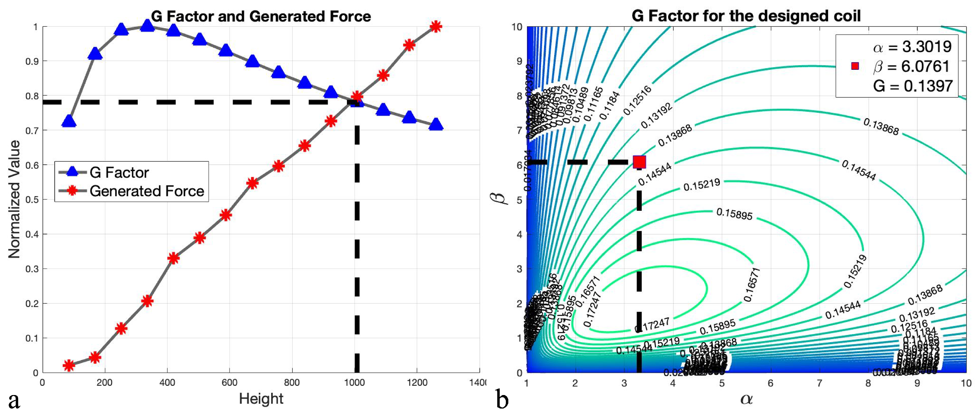
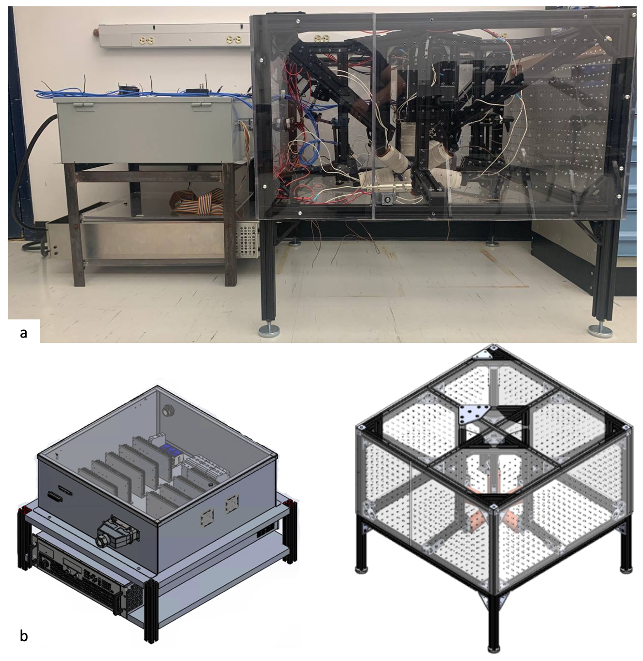
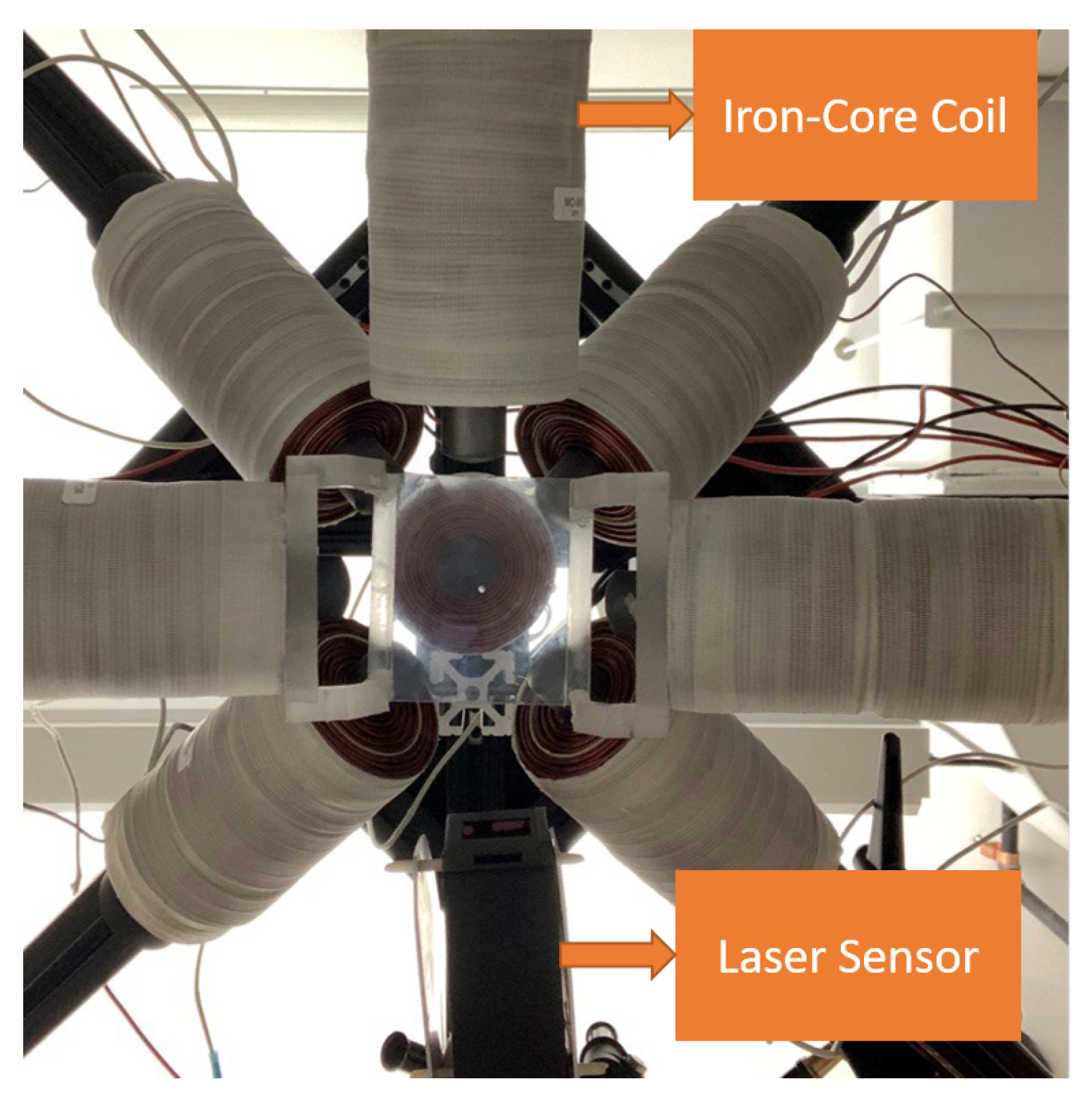
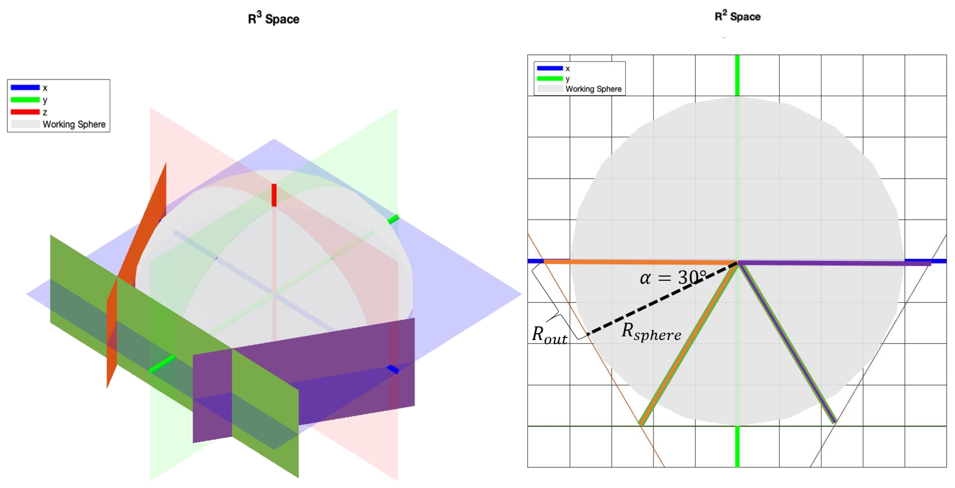
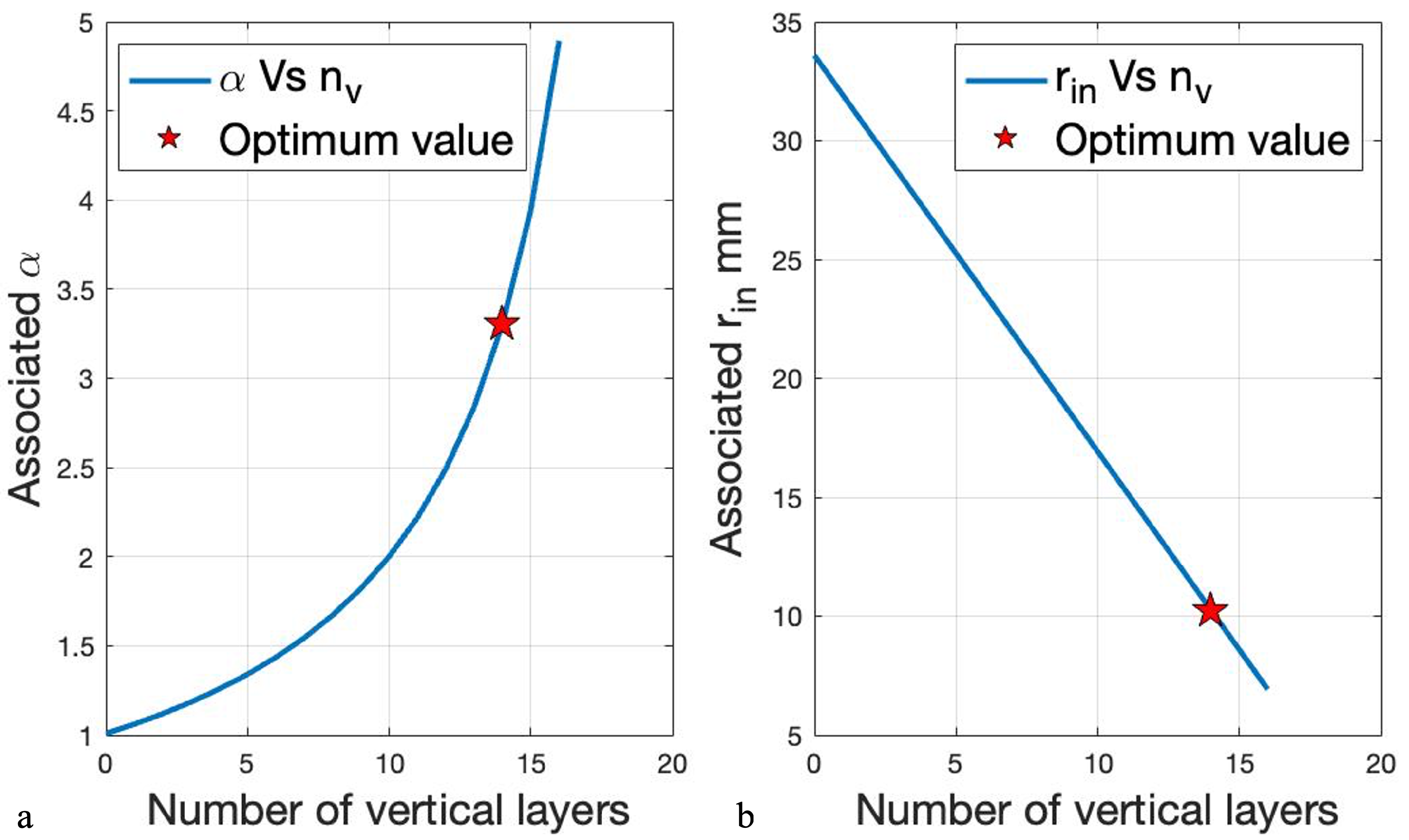
2.1. Coil Design
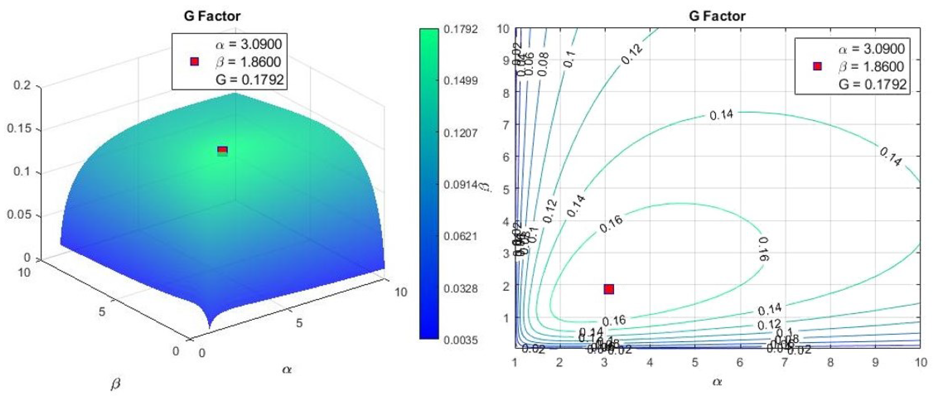
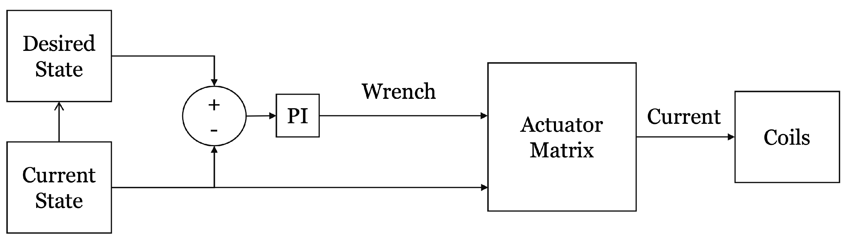
2.2. Magnetic Force and Torque
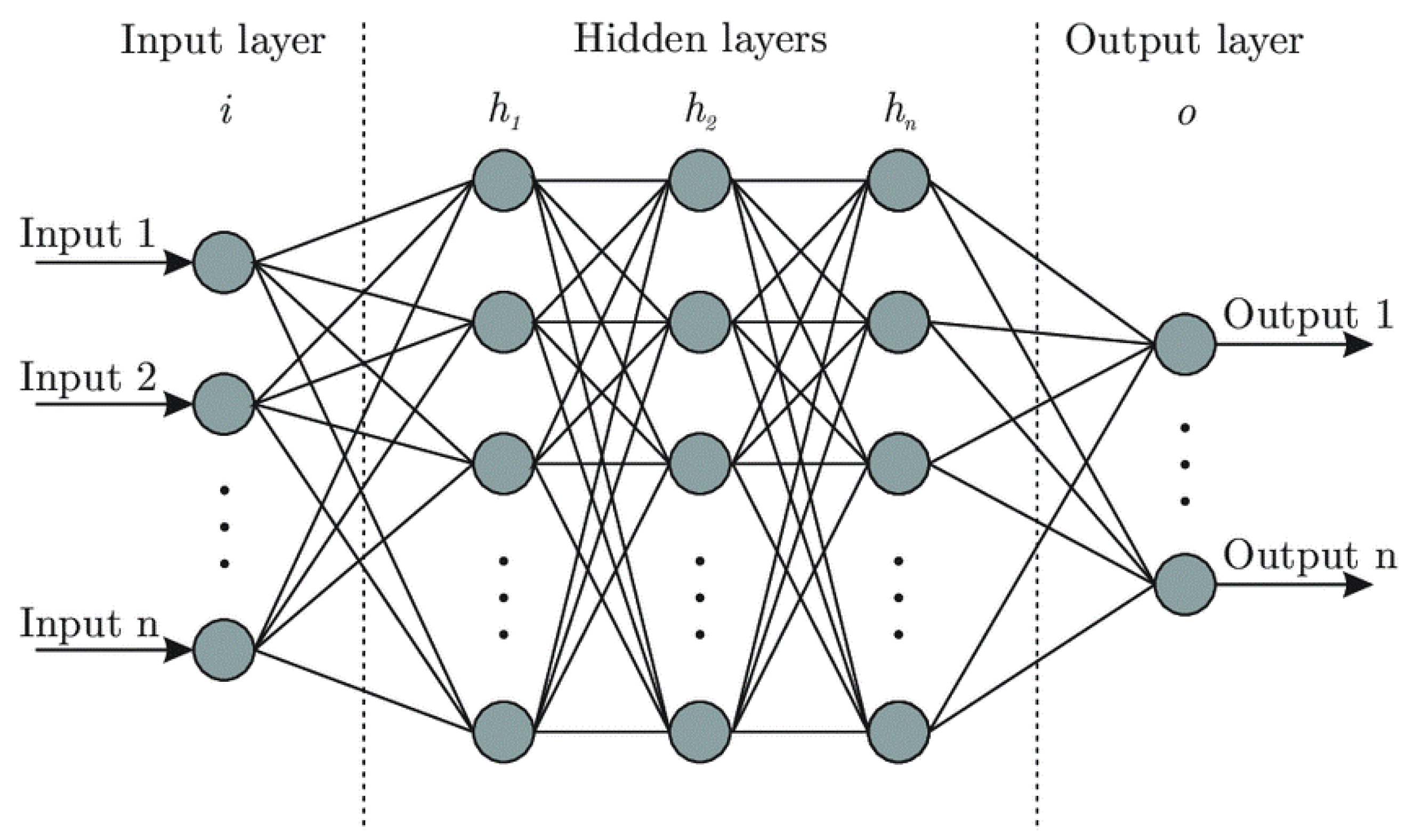
2.3. Deep Learning
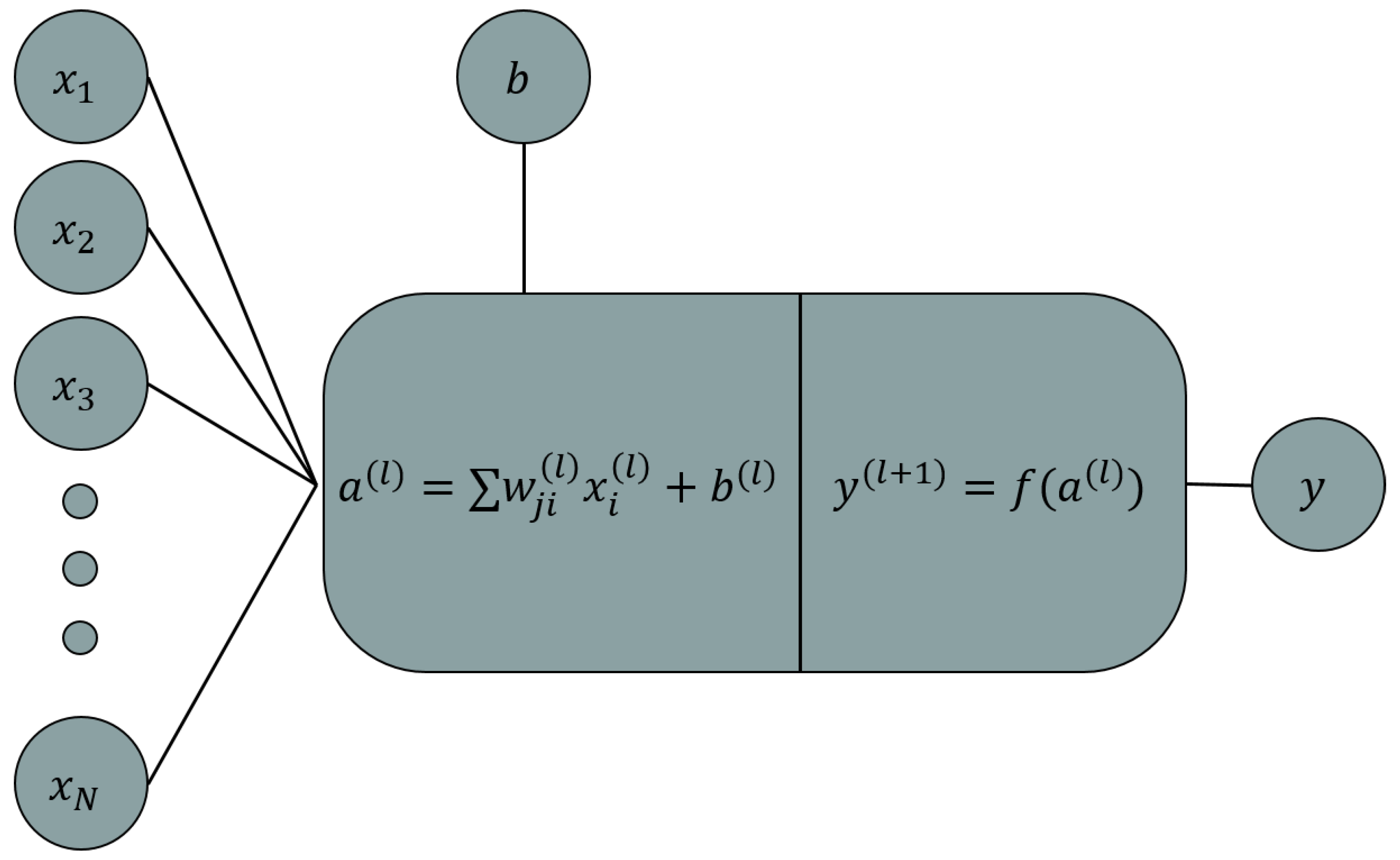
2.3.1. ANN
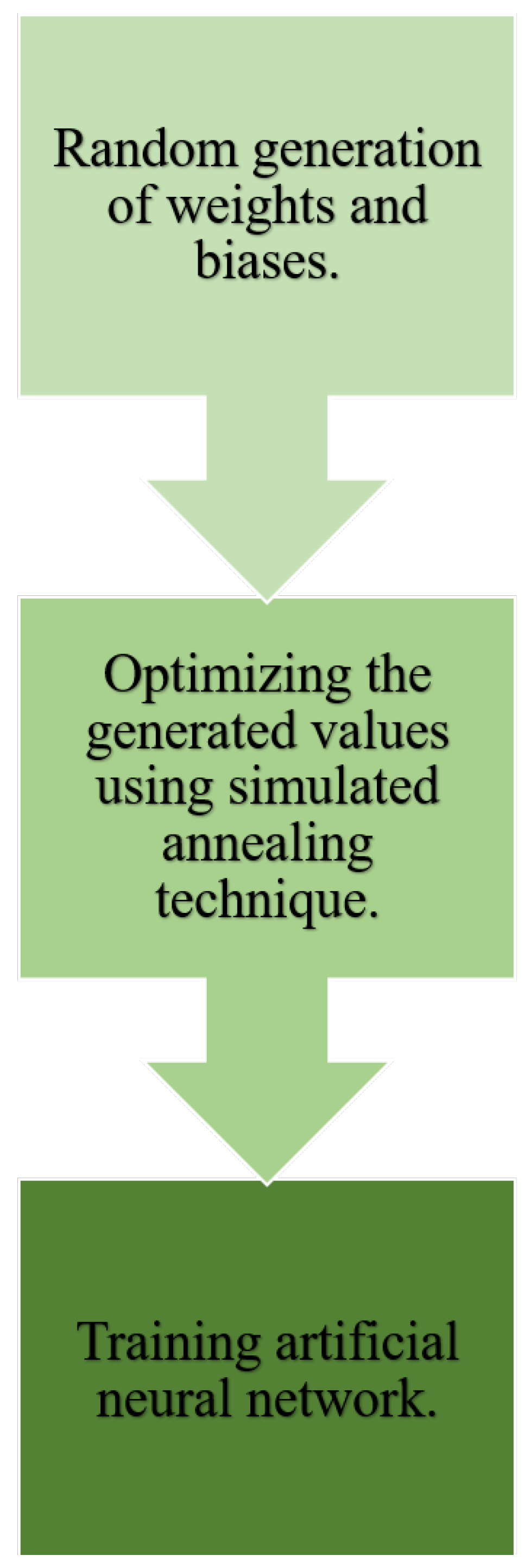
2.3.2. ANN/SA
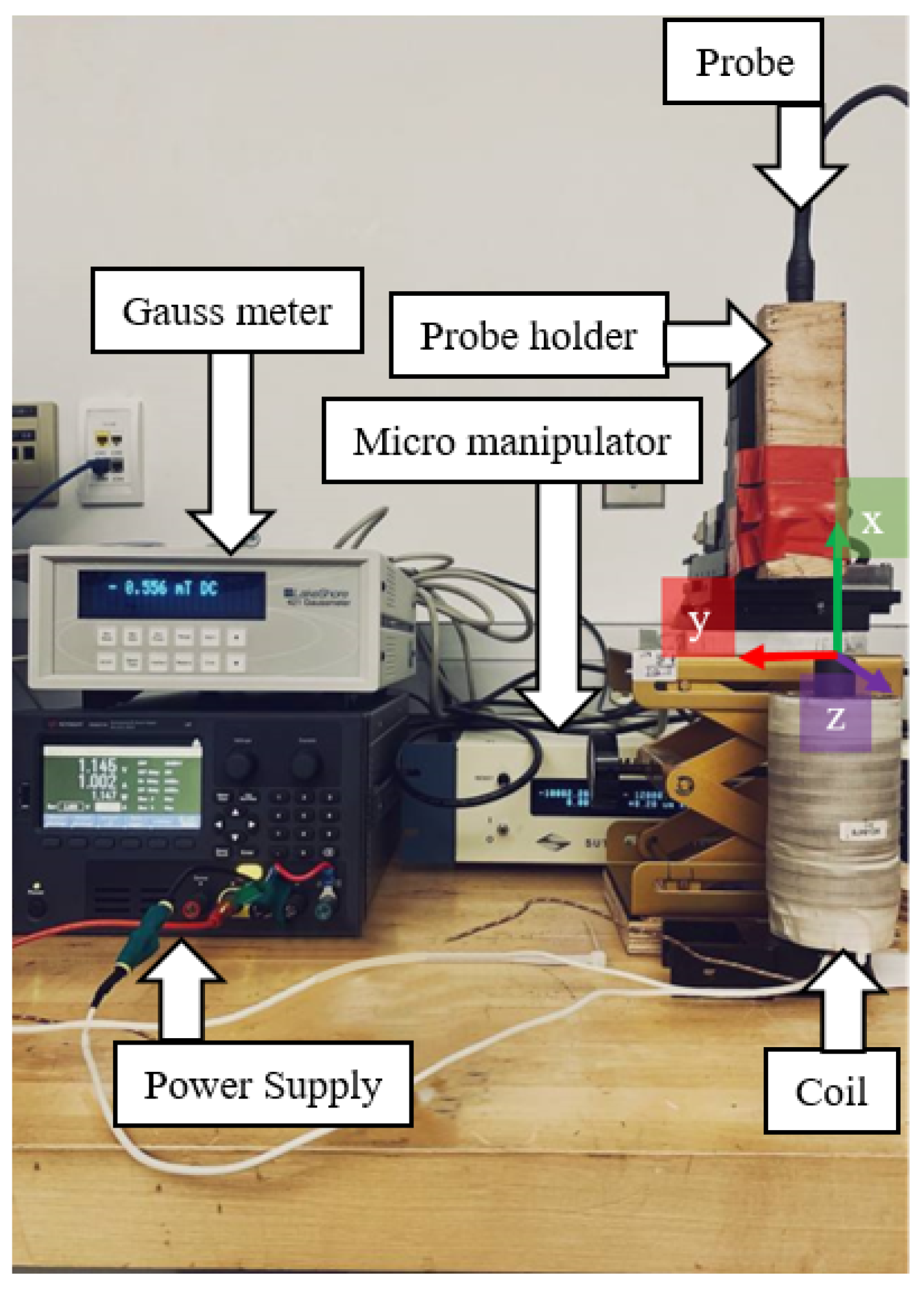
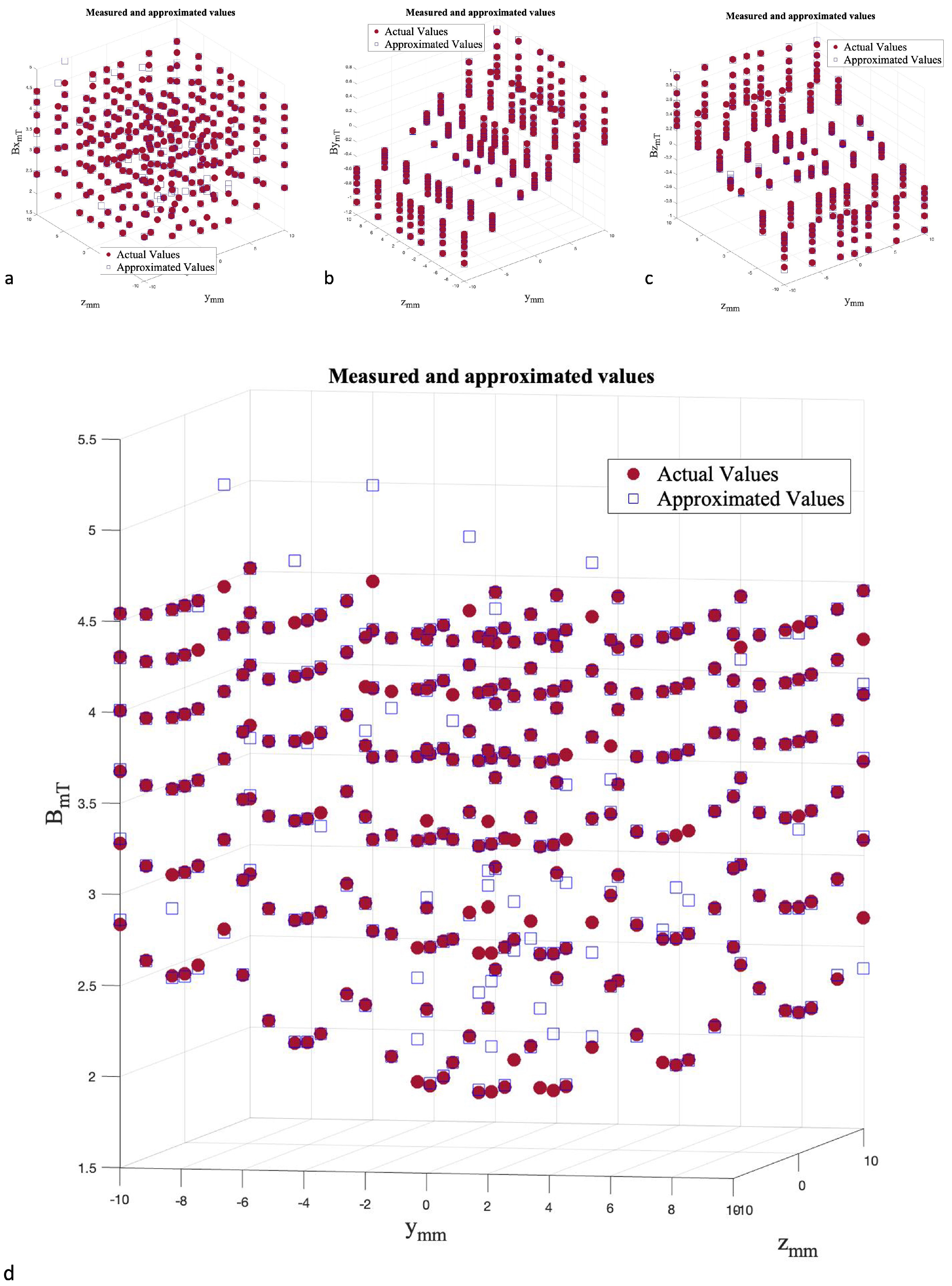
2.3.3. Validation
3. Results & Discussion
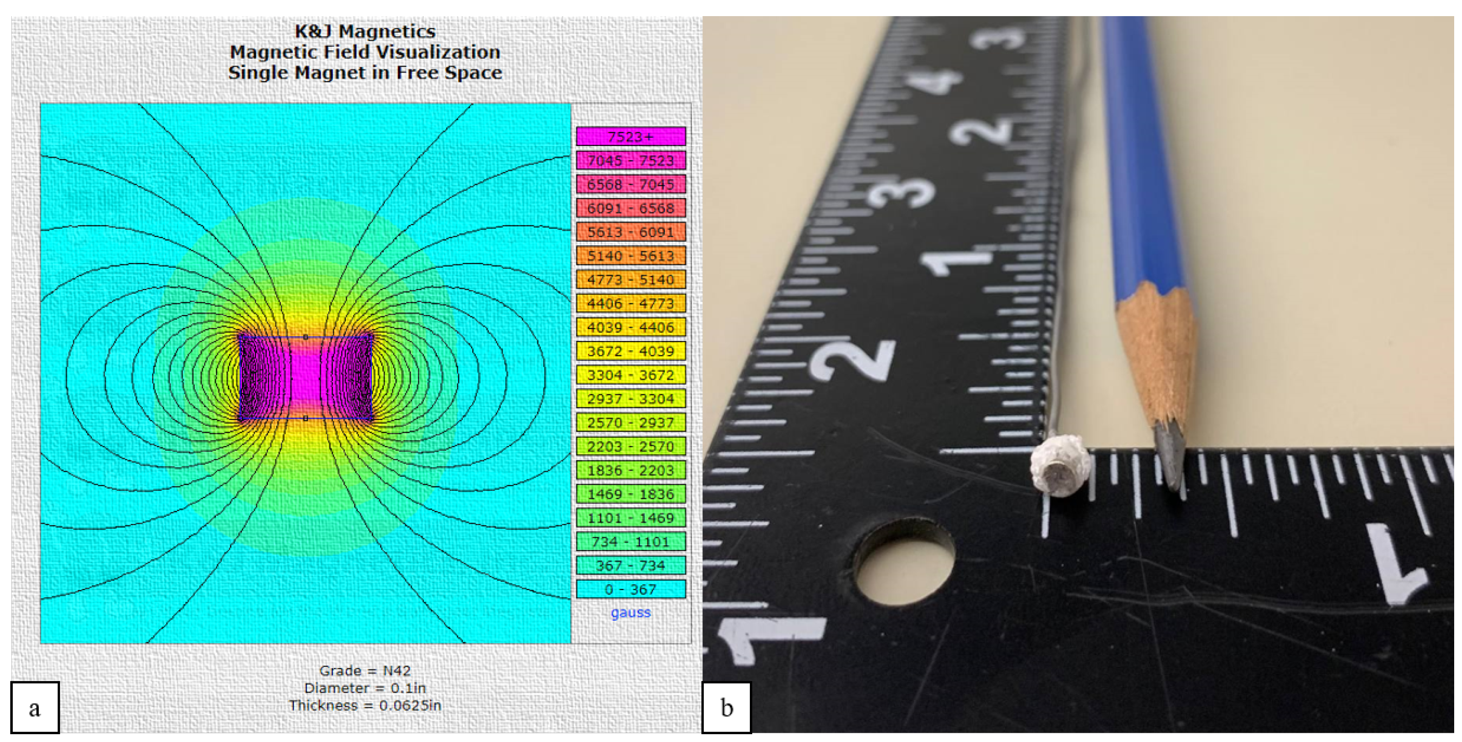
3.1. Designed Coil
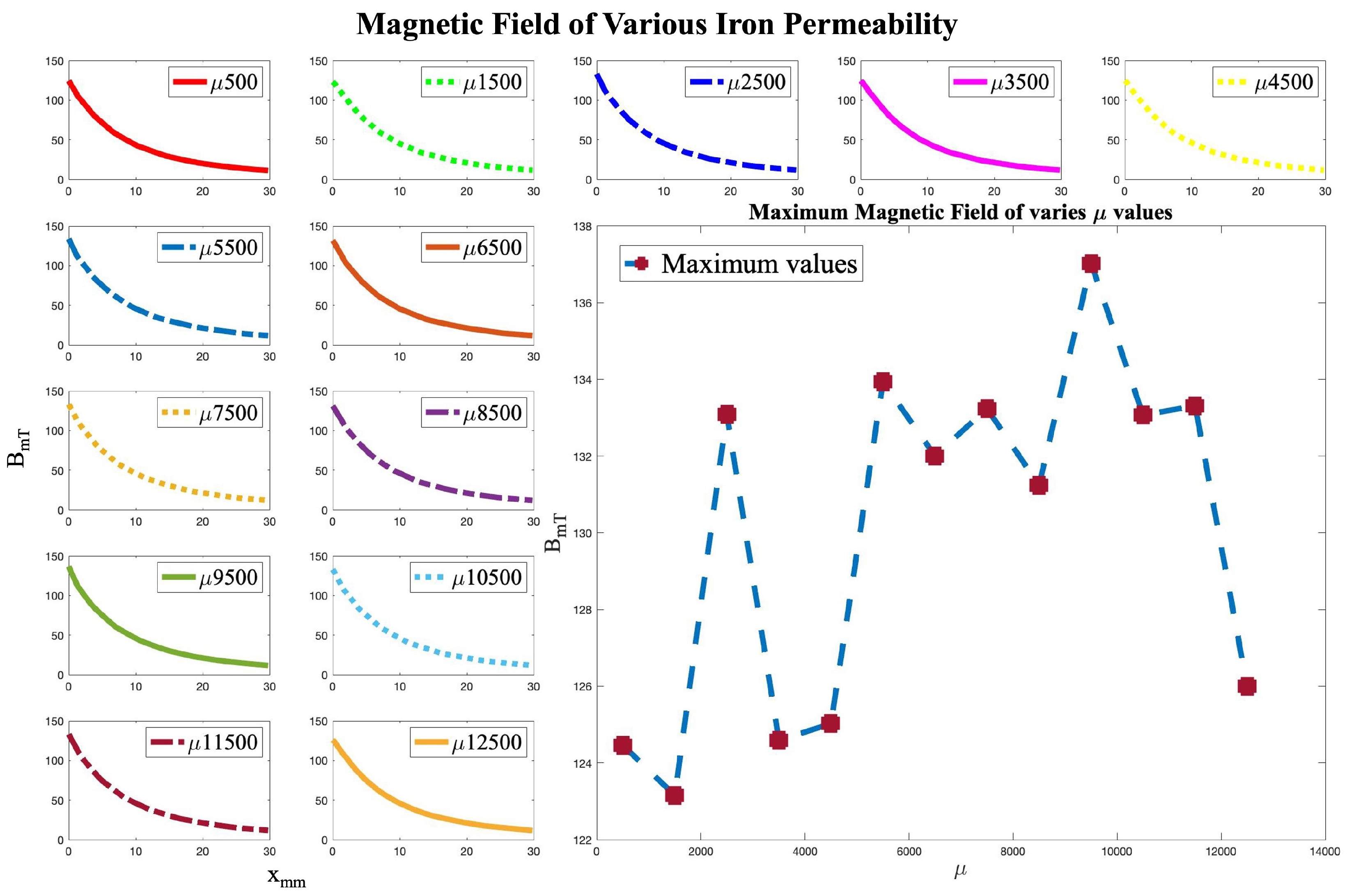
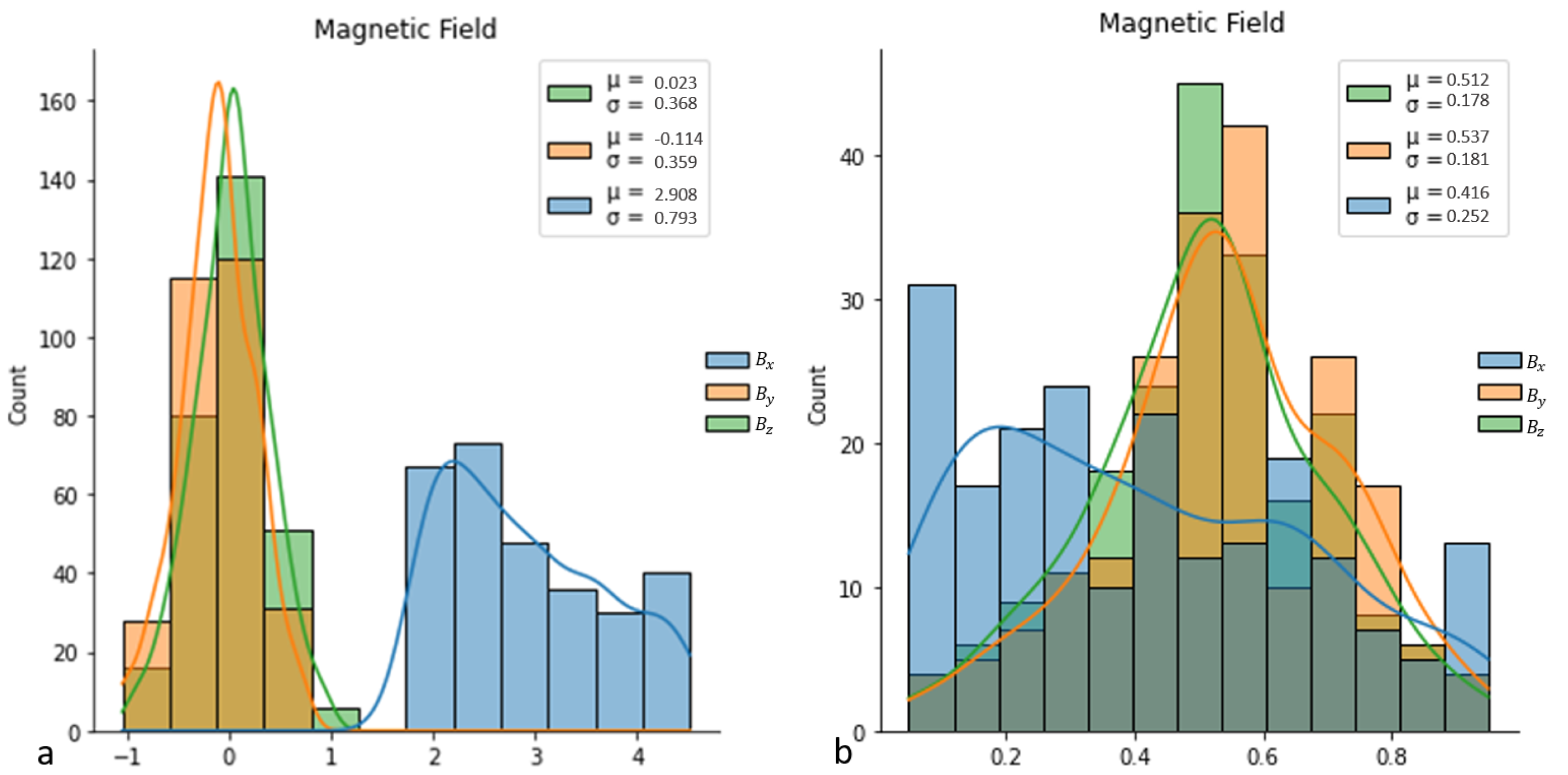
3.2. Data Collection
3.3. Algorithm Development
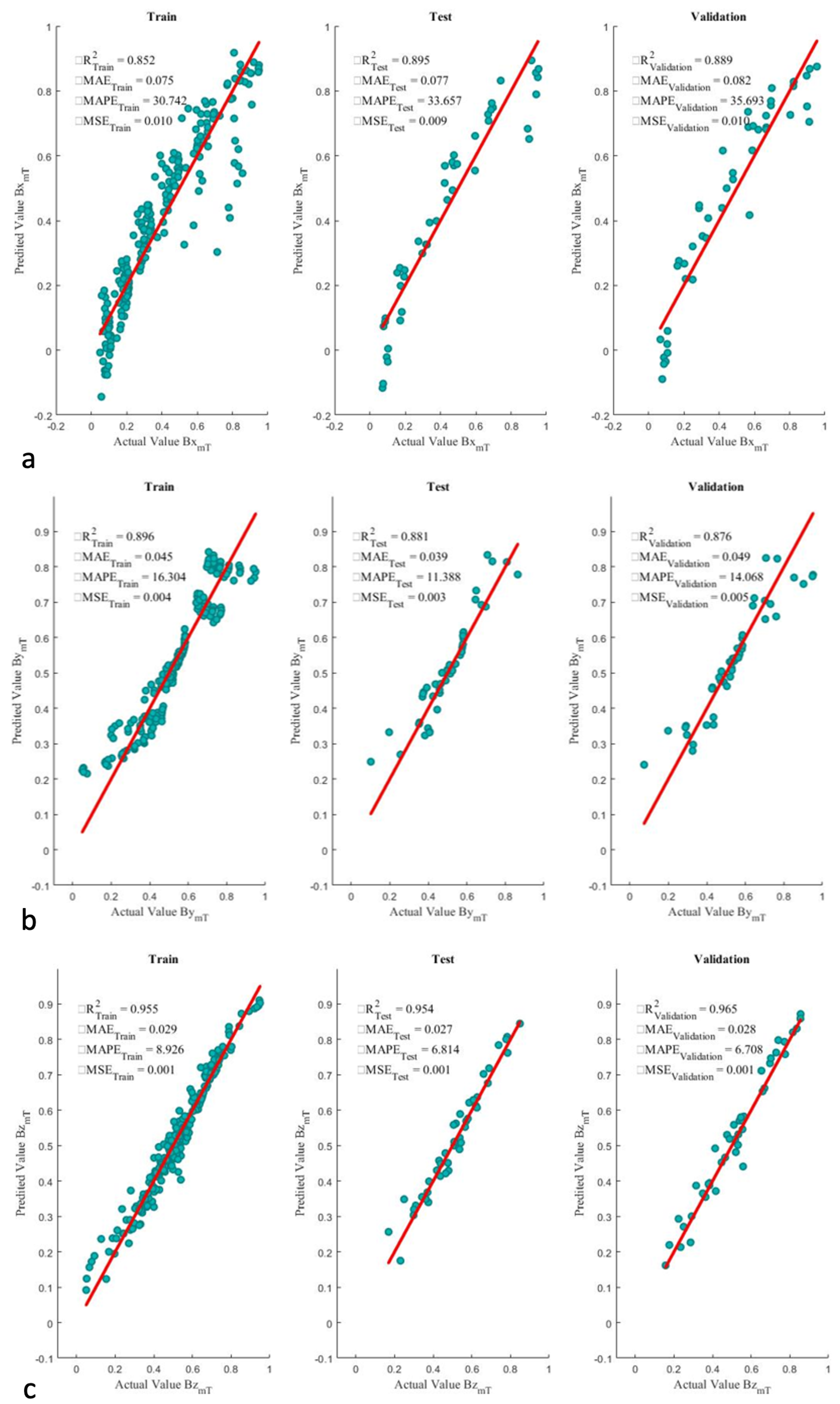
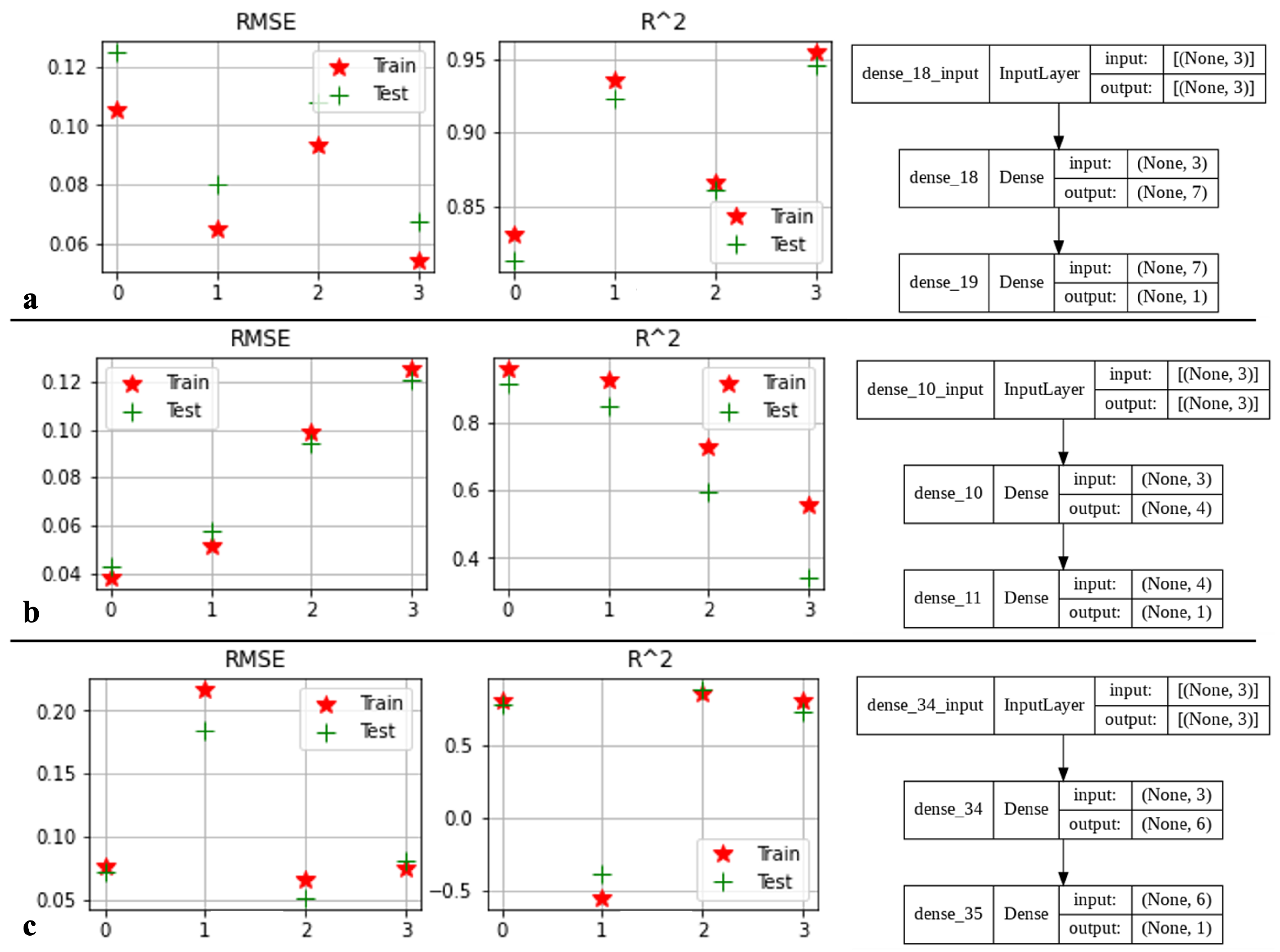
3.3.1. ANN
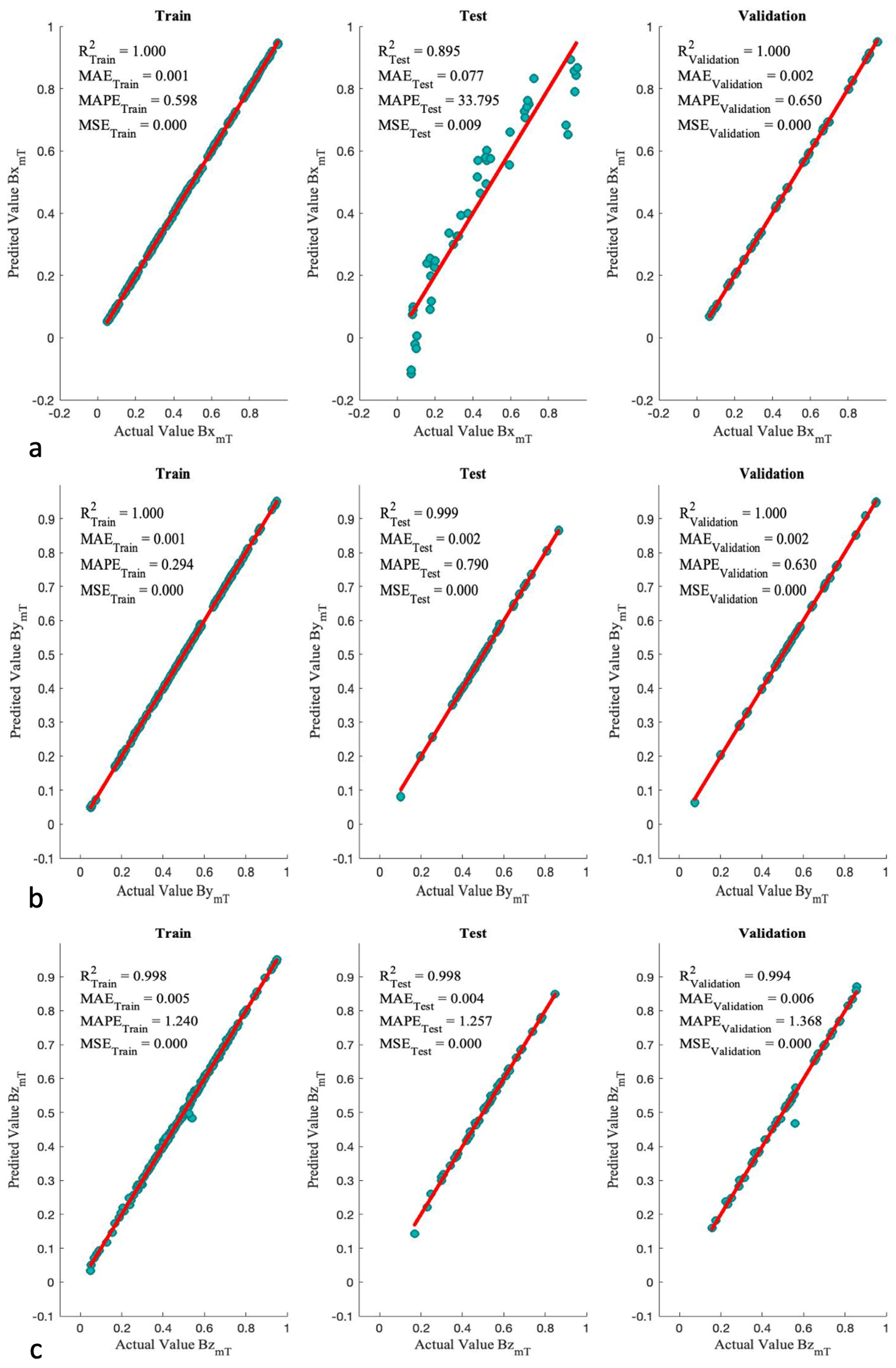
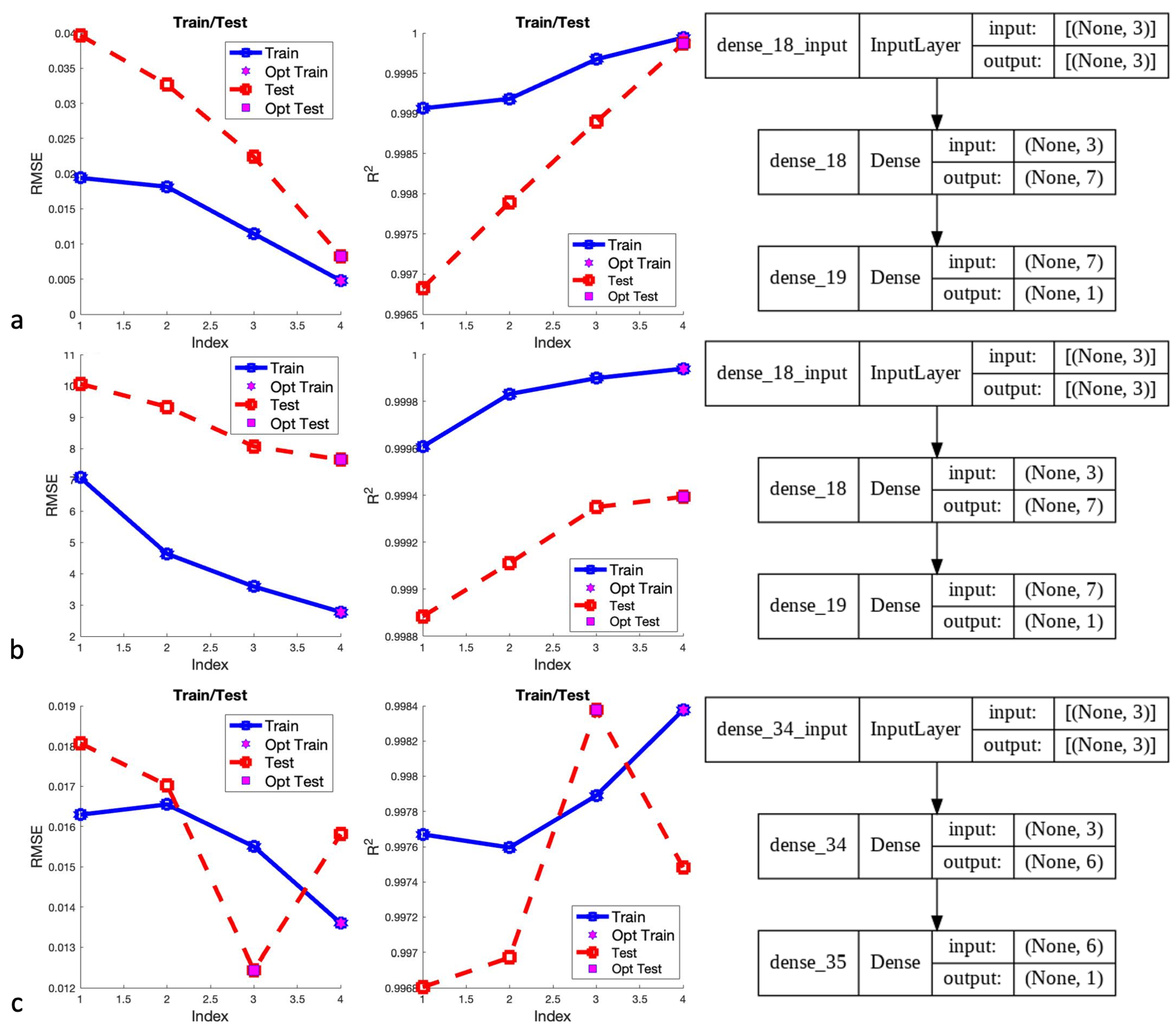
3.3.2. ANN/SA
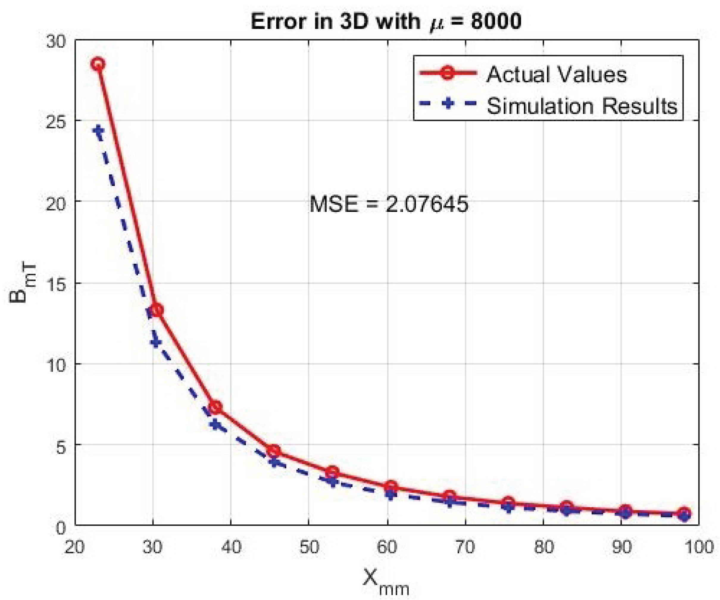
3.3.3. Extra Validation
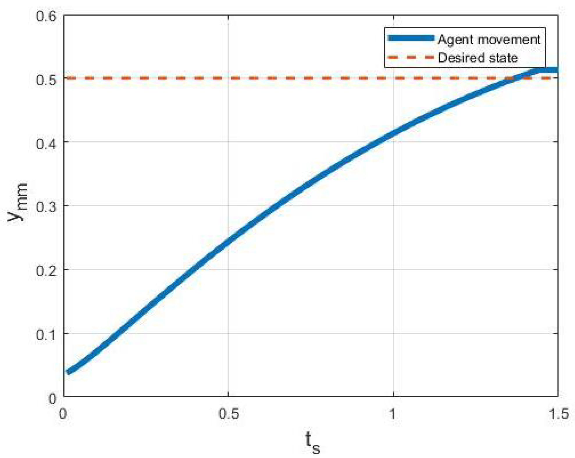
3.4. Motion
4. Conclusions
Author Contributions
Funding
Institutional Review Board Statement
Informed Consent Statement
Data Availability Statement
Conflicts of Interest
Abbreviations
| FEM | Finite Element Method |
| AI | Artificial Intelligence |
| ANN | Artificial Neural Network |
| ANN/SA | Artificial Neural Network with Simulated Annealing |
| DOF | Degrees Of Freedom |
| CGCI | Catheter Guidance Control and Imaging |
References
- Kamal, M.; Shang, J.; Cheng, V.; Hatkevich, S.; Daehn, G. Agile manufacturing of a micro-embossed case by a two-step electromagnetic forming process. J. Mater. Process. Technol. 2007, 190, 41–50. [Google Scholar] [CrossRef]
- Sarkar, A.; Somashekara, M.; Paranthaman, M.P.; Kramer, M.; Haase, C.; Nlebedim, I.C. Functionalizing magnet additive manufacturing with in-situ magnetic field source. Addit. Manuf. 2020, 34, 101289. [Google Scholar] [CrossRef]
- Kumar, P.; Huang, Y.; Toyserkani, E.; Khamesee, M.B. Development of a Magnetic Levitation System for Additive Manufacturing: Simulation Analyses. IEEE Trans. Magn. 2020, 56, 1–7. [Google Scholar] [CrossRef]
- Zandrini, T.; Taniguchi, S.; Maruo, S. Magnetically driven micromachines created by two-photon microfabrication and selective electroless magnetite plating for lab-on-a-chip applications. Micromachines 2017, 8, 35. [Google Scholar] [CrossRef] [Green Version]
- Lin, Y.T.; Huang, C.S.; Tseng, S.C. How to Control the Microfluidic Flow and Separate the Magnetic and Non-Magnetic Particles in the Runner of a Disc. Micromachines 2021, 12, 1335. [Google Scholar] [CrossRef]
- Li, X.; Meng, J.; Yang, C.; Zhang, H.; Zhang, L.; Song, R. A magnetically coupled electromagnetic energy harvester with low operating frequency for human body kinetic energy. Micromachines 2021, 12, 1300. [Google Scholar] [CrossRef]
- Jia, Y.; Zhao, P.; Xie, J.; Zhang, X.; Zhou, H.; Fu, J. Single-electromagnet levitation for density measurement and defect detection. Front. Mech. Eng. 2021, 16, 186–195. [Google Scholar] [CrossRef]
- Zhou, D.; Wang, J.; He, Y.; Chen, D.; Li, K. Influence of metallic shields on pulsed eddy current sensor for ferromagnetic materials defect detection. Sens. Actuators A Phys. 2016, 248, 162–172. [Google Scholar] [CrossRef]
- Shi, H.; Huo, D.; Zhang, H.; Li, W.; Sun, Y.; Li, G.; Chen, H. An Impedance Sensor for Distinguishing Multi-Contaminants in Hydraulic Oil of Offshore Machinery. Micromachines 2021, 12, 1407. [Google Scholar] [CrossRef]
- Nakai, T. Estimation of Position and Size of a Contaminant in Aluminum Casting Using a Thin-Film Magnetic Sensor. Micromachines 2022, 13, 127. [Google Scholar] [CrossRef]
- Qi, C.; Han, D.; Shinshi, T. A MEMS-based electromagnetic membrane actuator utilizing bonded magnets with large displacement. Sens. Actuators A Phys. 2021, 330, 112834. [Google Scholar] [CrossRef]
- Liu, D.; Liu, X.; Li, P.; Tang, X.; Kojima, M.; Huang, Q.; Arai, T. Magnetic Driven Two-Finger Micro-Hand with Soft Magnetic End-Effector for Force-Controlled Stable Manipulation in Microscale. Micromachines 2021, 12, 410. [Google Scholar] [CrossRef]
- Shameli, E.; Craig, D.G.; Khamesee, M.B. Design and implementation of a magnetically suspended microrobotic pick-and-place system. J. Appl. Phys. 2006, 99, 08P509. [Google Scholar] [CrossRef]
- Ştefănescu, D.M. Application of Electromagnetic and Optical Methods in Small Force Sensing. In Handbook of Force Transducers; Springer: Berlin/Heidelberg, Germany, 2020; pp. 41–50. [Google Scholar]
- Hong, D.K.; Lee, K.C.; Woo, B.C.; Koo, D.H. Optimum design of electromagnet in magnetic levitation system for contactless delivery application using response surface methodology. In Proceedings of the 2008 18th International Conference on Electrical Machines, Vilamoura, Portugal, 6–9 September 2008; pp. 1–6. [Google Scholar]
- Jeon, S.; Hoshiar, A.K.; Kim, K.; Lee, S.; Kim, E.; Lee, S.; Kim, J.Y.; Nelson, B.J.; Cha, H.J.; Yi, B.J.; et al. A magnetically controlled soft microrobot steering a guidewire in a three-dimensional phantom vascular network. Soft Robot. 2019, 6, 54–68. [Google Scholar] [CrossRef] [PubMed] [Green Version]
- Nelson, B.J.; Kaliakatsos, I.K.; Abbott, J.J. Microrobots for minimally invasive medicine. Annu. Rev. Biomed. Eng. 2010, 12, 55–85. [Google Scholar] [CrossRef] [PubMed] [Green Version]
- Zhang, J. Evolving from laboratory toys towards life-savers: Small-scale magnetic robotic systems with medical imaging modalities. Micromachines 2021, 12, 1310. [Google Scholar] [CrossRef]
- Giltinan, J.; Sitti, M. Simultaneous six-degree-of-freedom control of a single-body magnetic microrobot. IEEE Robot. Autom. Lett. 2019, 4, 508–514. [Google Scholar] [CrossRef]
- Sitti, M.; Ceylan, H.; Hu, W.; Giltinan, J.; Turan, M.; Yim, S.; Diller, E. Biomedical applications of untethered mobile milli/microrobots. Proc. IEEE 2015, 103, 205–224. [Google Scholar] [CrossRef]
- Kummer, M.P.; Abbott, J.J.; Kratochvil, B.E.; Borer, R.; Sengul, A.; Nelson, B.J. OctoMag: An electromagnetic system for 5-DOF wireless micromanipulation. IEEE Trans. Robot. 2010, 26, 1006–1017. [Google Scholar] [CrossRef]
- Yuan, S.; Wan, Y.; Mao, Y.; Song, S.; Meng, M.Q.H. Design of a novel electromagnetic actuation system for actuating magnetic capsule robot. In Proceedings of the 2019 IEEE International Conference on Robotics and Biomimetics (ROBIO), Dali, China, 6–8 December 2019; pp. 1513–1519. [Google Scholar]
- Cole, G.A.; Harrington, K.; Su, H.; Camilo, A.; Pilitsis, J.G.; Fischer, G.S. Closed-loop actuated surgical system utilizing real-time in-situ MRI guidance. In Experimental Robotics; Springer: Berlin/Heidelberg, Germany, 2014; pp. 785–798. [Google Scholar]
- Le, V.N.; Nguyen, N.H.; Alameh, K.; Weerasooriya, R.; Pratten, P. Accurate modeling and positioning of a magnetically controlled catheter tip. Med. Phys. 2016, 43, 650–663. [Google Scholar] [CrossRef]
- Edelmann, J.; Petruska, A.J.; Nelson, B.J. Estimation-based control of a magnetic endoscope without device localization. J. Med. Robot. Res. 2018, 3, 1850002. [Google Scholar] [CrossRef]
- Nguyen, B.L.; Merino, J.L.; Gang, E.S. Remote navigation for ablation procedures—A new step forward in the treatment of cardiac arrhythmias. Eur. Cardiol. 2010, 6, 50–56. [Google Scholar] [CrossRef]
- Sikorski, J.; Dawson, I.; Denasi, A.; Hekman, E.E.; Misra, S. Introducing BigMag—A novel system for 3D magnetic actuation of flexible surgical manipulators. In Proceedings of the 2017 IEEE International Conference on Robotics and Automation (ICRA), Singapore, 29 May–3 June 2017; pp. 3594–3599. [Google Scholar]
- Pourkand, A.; Abbott, J.J. A critical analysis of eight-electromagnet manipulation systems: The role of electromagnet configuration on strength, isotropy, and access. IEEE Robot. Autom. Lett. 2018, 3, 2957–2962. [Google Scholar] [CrossRef]
- Thomson, J.J. XXIV. On the structure of the atom: An investigation of the stability and periods of oscillation of a number of corpuscles arranged at equal intervals around the circumference of a circle; with application of the results to the theory of atomic structure. Lond. Edinb. Dublin Philos. Mag. J. Sci. 1904, 7, 237–265. [Google Scholar] [CrossRef] [Green Version]
- Petruska, A.J.; Nelson, B.J. Minimum bounds on the number of electromagnets required for remote magnetic manipulation. IEEE Trans. Robot. 2015, 31, 714–722. [Google Scholar] [CrossRef]
- Yu, Q.; Tang, H.; Tan, K.C.; Yu, H. A brain-inspired spiking neural network model with temporal encoding and learning. Neurocomputing 2014, 138, 3–13. [Google Scholar] [CrossRef]
- Put, R.; Perrin, C.; Questier, F.; Coomans, D.; Massart, D.; Vander Heyden, Y. Classification and regression tree analysis for molecular descriptor selection and retention prediction in chromatographic quantitative structure–retention relationship studies. J. Chromatogr. A 2003, 988, 261–276. [Google Scholar] [CrossRef]
- Dongare, A.; Kharde, R.; Kachare, A.D. Introduction to artificial neural network. Int. J. Eng. Innov. Technol. 2012, 2, 189–194. [Google Scholar]
- Alaloul, W.S.; Qureshi, A.H. Data processing using artificial neural network. In Dynamic Data Assimilation-Beating the Uncertainties; IntechOpen: London, UK, 2020. [Google Scholar]
- Abramson, D.; Krishnamoorthy, M.; Dang, H. Simulated annealing cooling schedules for the school timetabling problem. Asia Pac. J. Oper. Res. 1999, 16, 1–22. [Google Scholar]
- Alavi, A.H.; Ameri, M.; Gandomi, A.H.; Mirzahosseini, M.R. Formulation of flow number of asphalt mixes using a hybrid computational method. Constr. Build. Mater. 2011, 25, 1338–1355. [Google Scholar] [CrossRef]
- Gandomi, A.H.; Alavi, A.H.; Shadmehri, D.M.; Sahab, M. An empirical model for shear capacity of RC deep beams using genetic-simulated annealing. Arch. Civ. Mech. Eng. 2013, 13, 354–369. [Google Scholar] [CrossRef]
- Alavi, A.H.; Gandomi, A.H. Prediction of principal ground-motion parameters using a hybrid method coupling artificial neural networks and simulated annealing. Comput. Struct. 2011, 89, 2176–2194. [Google Scholar] [CrossRef]
- Golbraikh, A.; Tropsha, A. Predictive QSAR modeling based on diversity sampling of experimental datasets for the training and test set selection. Mol. Divers. 2000, 5, 231–243. [Google Scholar] [CrossRef] [PubMed]
- Golbraikh, A.; Tropsha, A. Beware of q2! J. Mol. Graph. Model. 2002, 20, 269–276. [Google Scholar] [CrossRef]
- Magnetics, K. Single Magnet in Free Space. Available online: https://www.kjmagnetics.com/magfield.asp?D=0.1&T=0.0625&L=&W=&OD=&ID=&calcType=disc&GRADE=42&surf_field=5154&rsurfC=&rsurfR= (accessed on 10 December 2021).


| Variable | Equation | Criteria |
|---|---|---|
| Mean Absolute Error (MAE) | As low as possible | |
| Mean Absolute Percentage Error (MAPE) | As low as possible | |
| Slope regression line k | k = | |
| Slope regression line | ||
| Squared correlation of actual vs predicted | = | Close to 1 |
| Squared correlation of predicted vs actual | = | Close to 1 |
| Predictability of model | = | |
| Performance index m | m = | |
| Performance index n | n = |
| Lengthmm | G | ForcemT | |
|---|---|---|---|
| 10.38 | 0.5063 | 0.129 | 0.013 |
| 20.76 | 1.0127 | 0.164 | 0.027 |
| 31.14 | 1.5190 | 0.177 | 0.080 |
| 41.52 | 2.0254 | 0.179 | 0.129 |
| 51.90 | 2.5317 | 0.176 | 0.207 |
| 62.28 | 3.0380 | 0.172 | 0.243 |
| 72.66 | 3.5444 | 0.166 | 0.284 |
| 83.04 | 4.0507 | 0.160 | 0.342 |
| 93.42 | 4.5571 | 0.155 | 0.373 |
| 103.80 | 5.0634 | 0.149 | 0.409 |
| 114.18 | 5.5698 | 0.144 | 0.454 |
| 124.56 | 6.0761 | 0.140 | 0.497 |
| 134.94 | 6.5824 | 0.135 | 0.536 |
| 145.32 | 7.0888 | 0.131 | 0.591 |
| 155.70 | 7.5951 | 0.128 | 0.625 |
| Variable | Criteria | |||
|---|---|---|---|---|
| k | 0.9995 | 0.9988 | 0.9985 | |
| 1.0005 | 1.0012 | 1.0007 | ||
| 1.0000 | 1.0000 | 1.0000 | Close to 1 | |
| 1.0000 | 1.0000 | 1.0000 | Close to 1 | |
| 0.9912 | 0.9867 | 0.9161 | ||
| m | −0.0001 | −0.0062 | ||
| n | −0.0001 | −0.0062 |
Publisher’s Note: MDPI stays neutral with regard to jurisdictional claims in published maps and institutional affiliations. |
© 2022 by the authors. Licensee MDPI, Basel, Switzerland. This article is an open access article distributed under the terms and conditions of the Creative Commons Attribution (CC BY) license (https://creativecommons.org/licenses/by/4.0/).
Share and Cite
Kazemzadeh Heris, P.; Khamesee, M.B. Design and Fabrication of a Magnetic Actuator for Torque and Force Control Estimated by the ANN/SA Algorithm. Micromachines 2022, 13, 327. https://doi.org/10.3390/mi13020327
Kazemzadeh Heris P, Khamesee MB. Design and Fabrication of a Magnetic Actuator for Torque and Force Control Estimated by the ANN/SA Algorithm. Micromachines. 2022; 13(2):327. https://doi.org/10.3390/mi13020327
Chicago/Turabian StyleKazemzadeh Heris, Pooriya, and Mir Behrad Khamesee. 2022. "Design and Fabrication of a Magnetic Actuator for Torque and Force Control Estimated by the ANN/SA Algorithm" Micromachines 13, no. 2: 327. https://doi.org/10.3390/mi13020327
APA StyleKazemzadeh Heris, P., & Khamesee, M. B. (2022). Design and Fabrication of a Magnetic Actuator for Torque and Force Control Estimated by the ANN/SA Algorithm. Micromachines, 13(2), 327. https://doi.org/10.3390/mi13020327