
Numerical Computation for Gyrotactic Microorganisms in MHD Radiative Eyring–Powell Nanomaterial Flow by a Static/Moving Wedge with Darcy–Forchheimer Relation

 , , , , , , and
Abstract
1. Introduction
2. Materials Formulation
Engineering Quantities
3. Solution Strategy
4. Result and Analysis
5. Final Remarks
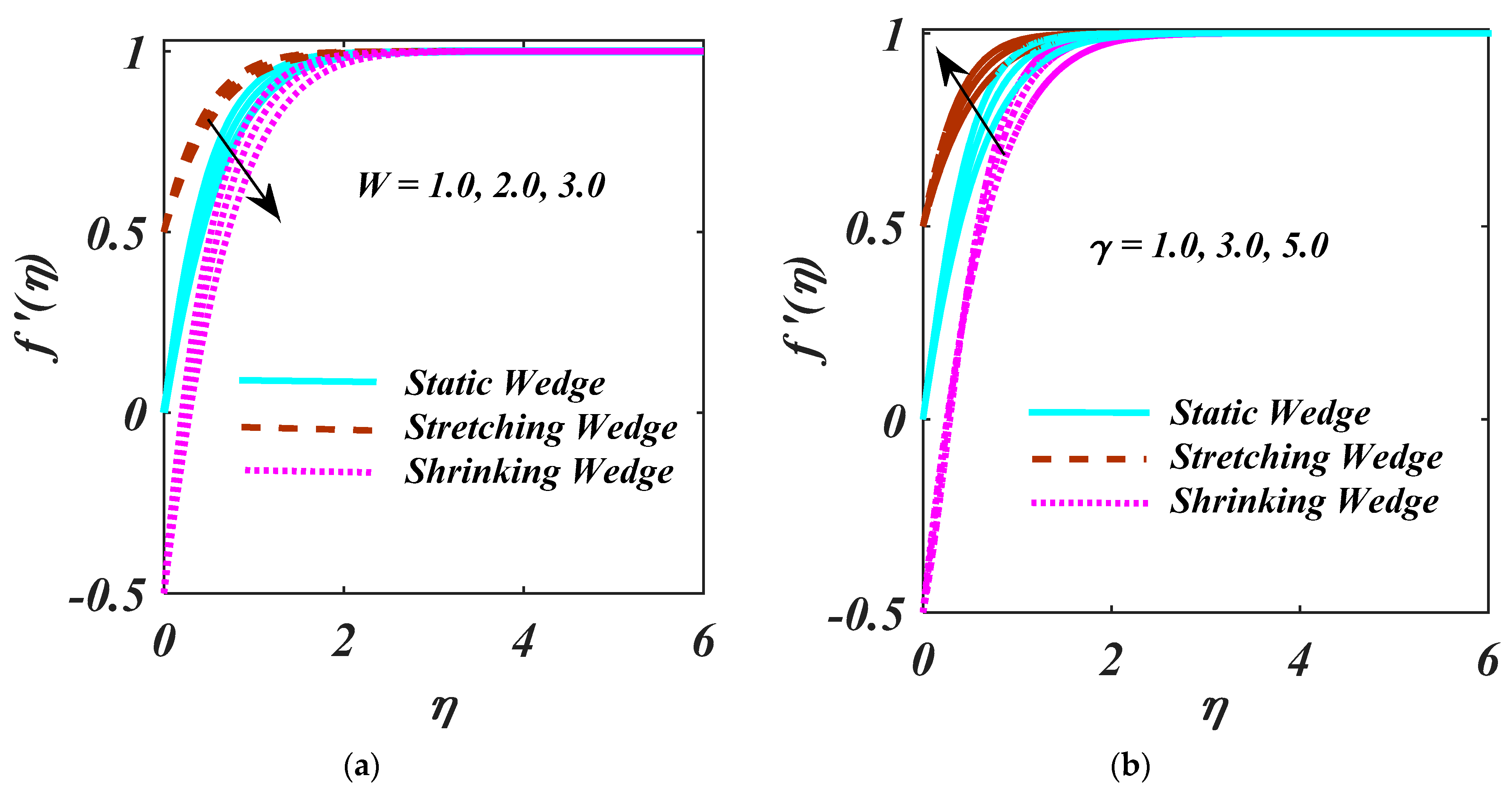
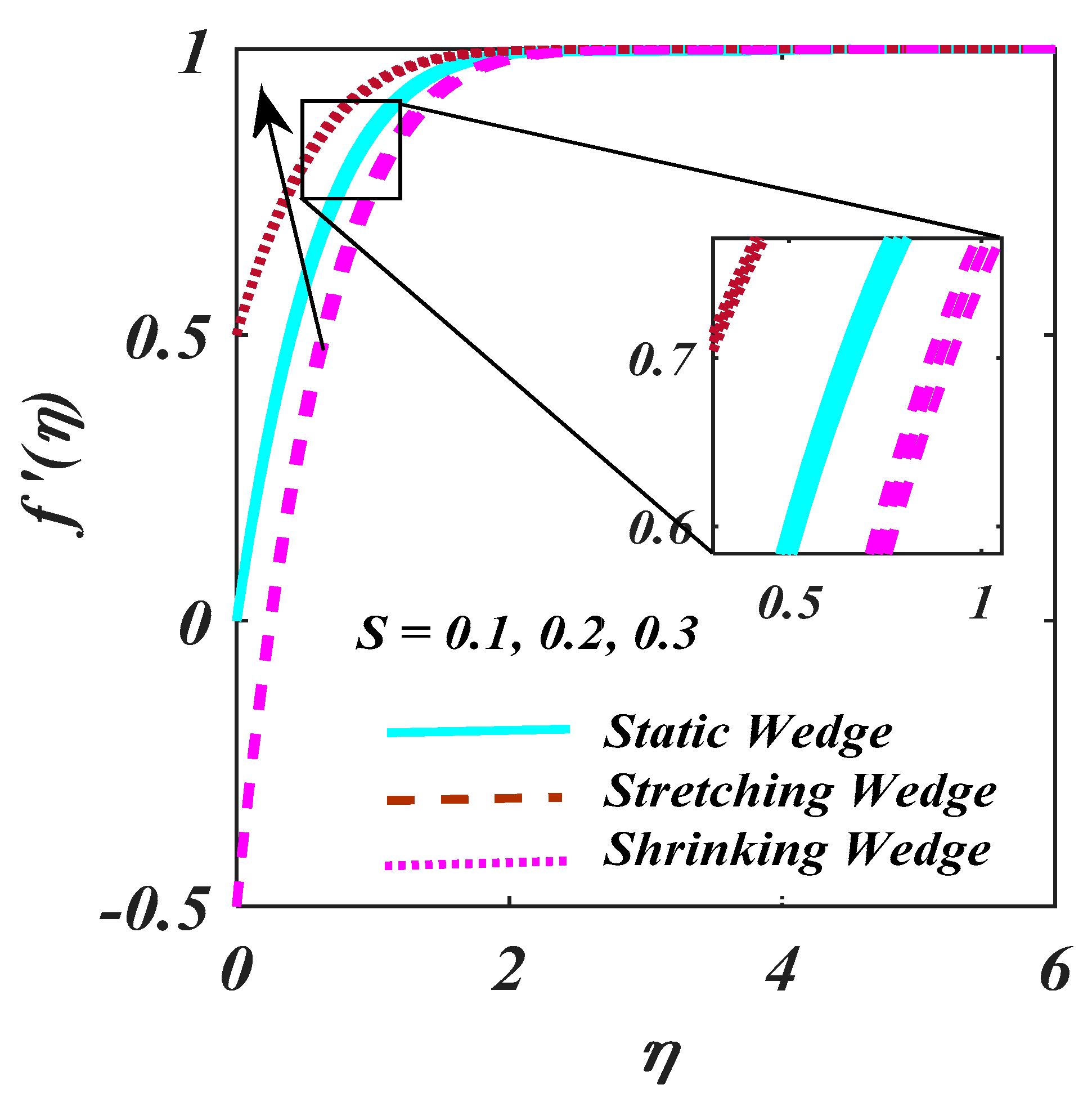
- Larger values of and shrink the velocity profile.
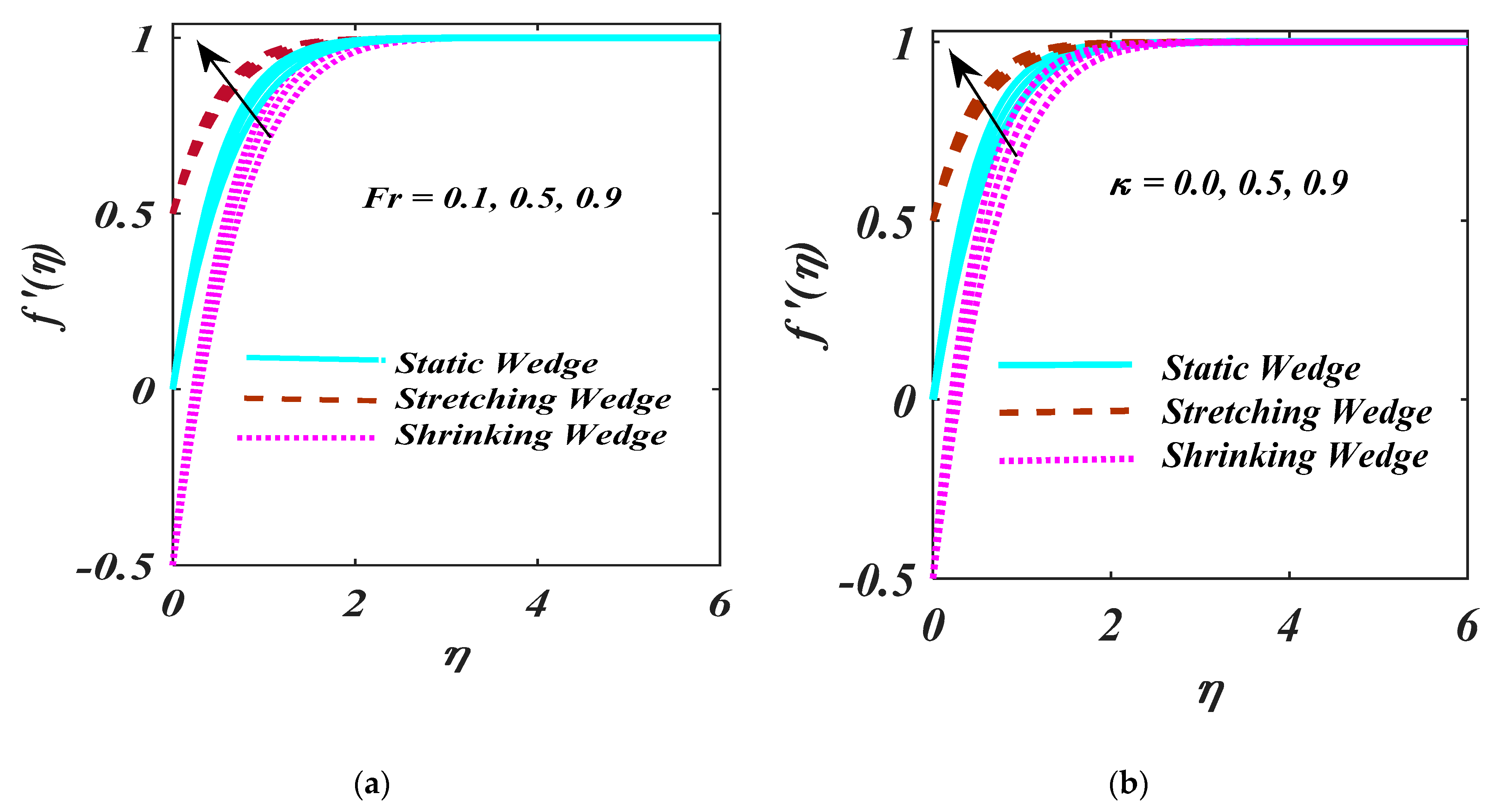
- A larger Forchheimer number depicts the decreasing behaviour for the velocity profile.
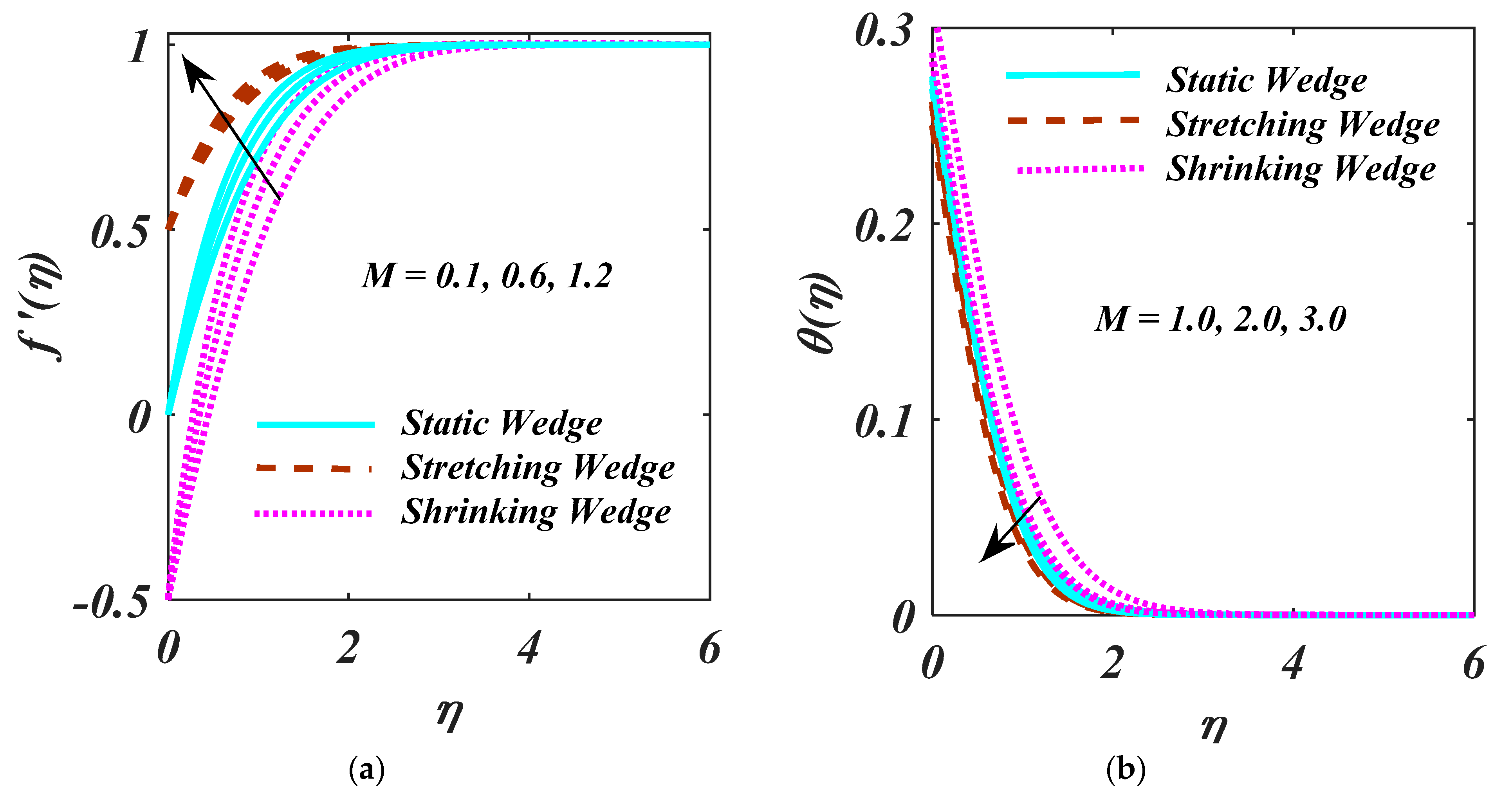
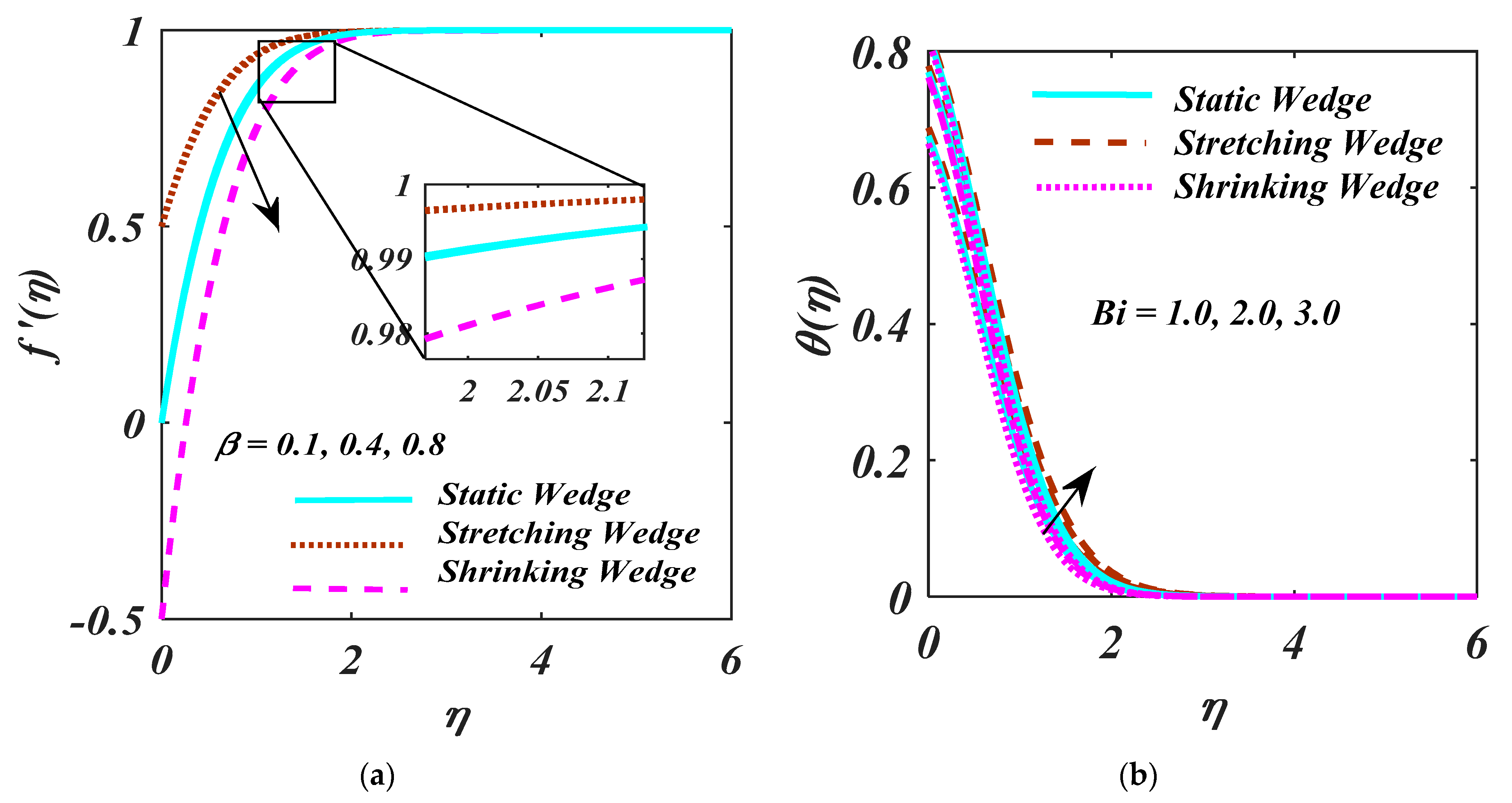
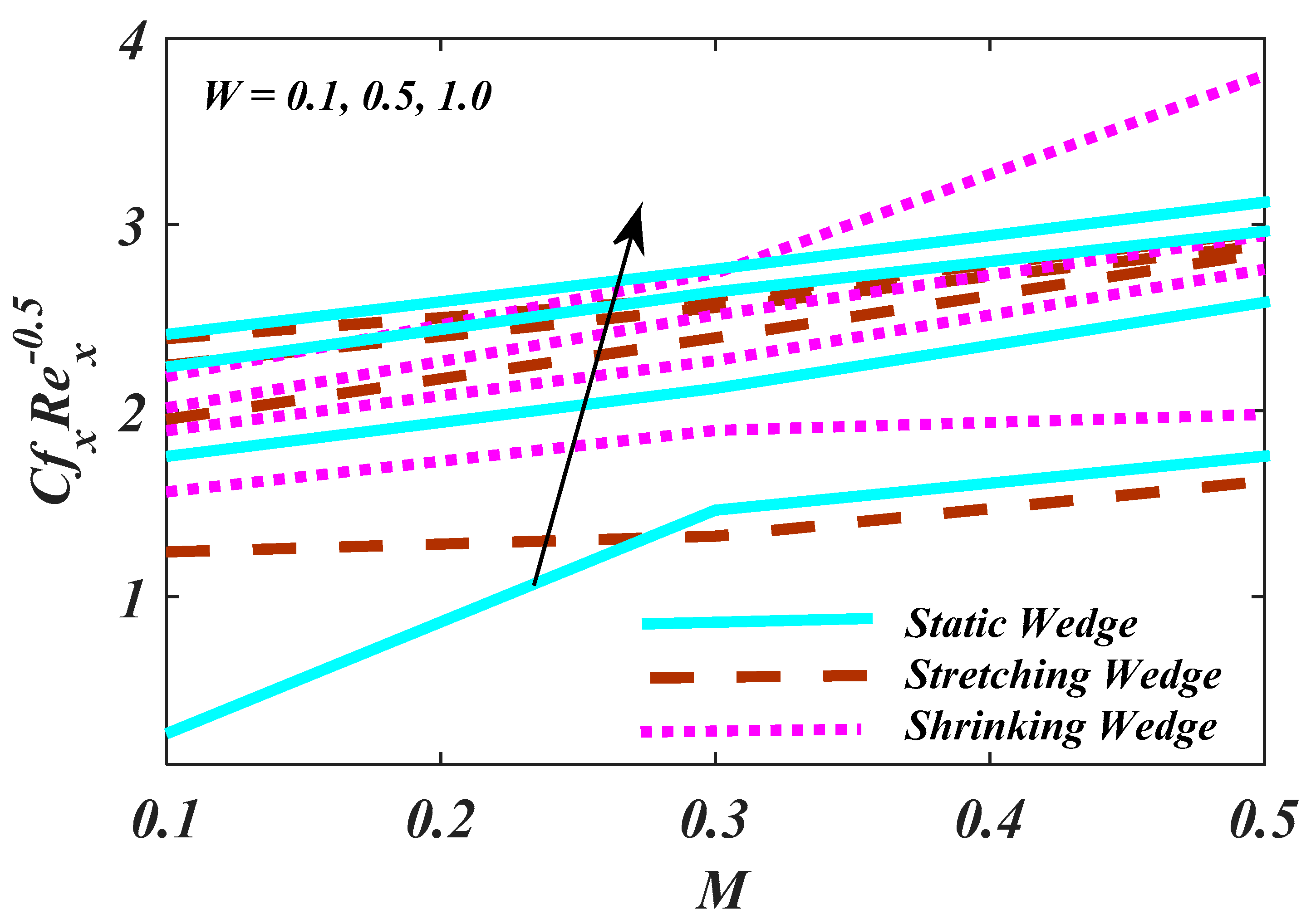
- Rising values of M enhance the stretching wedge of velocity.
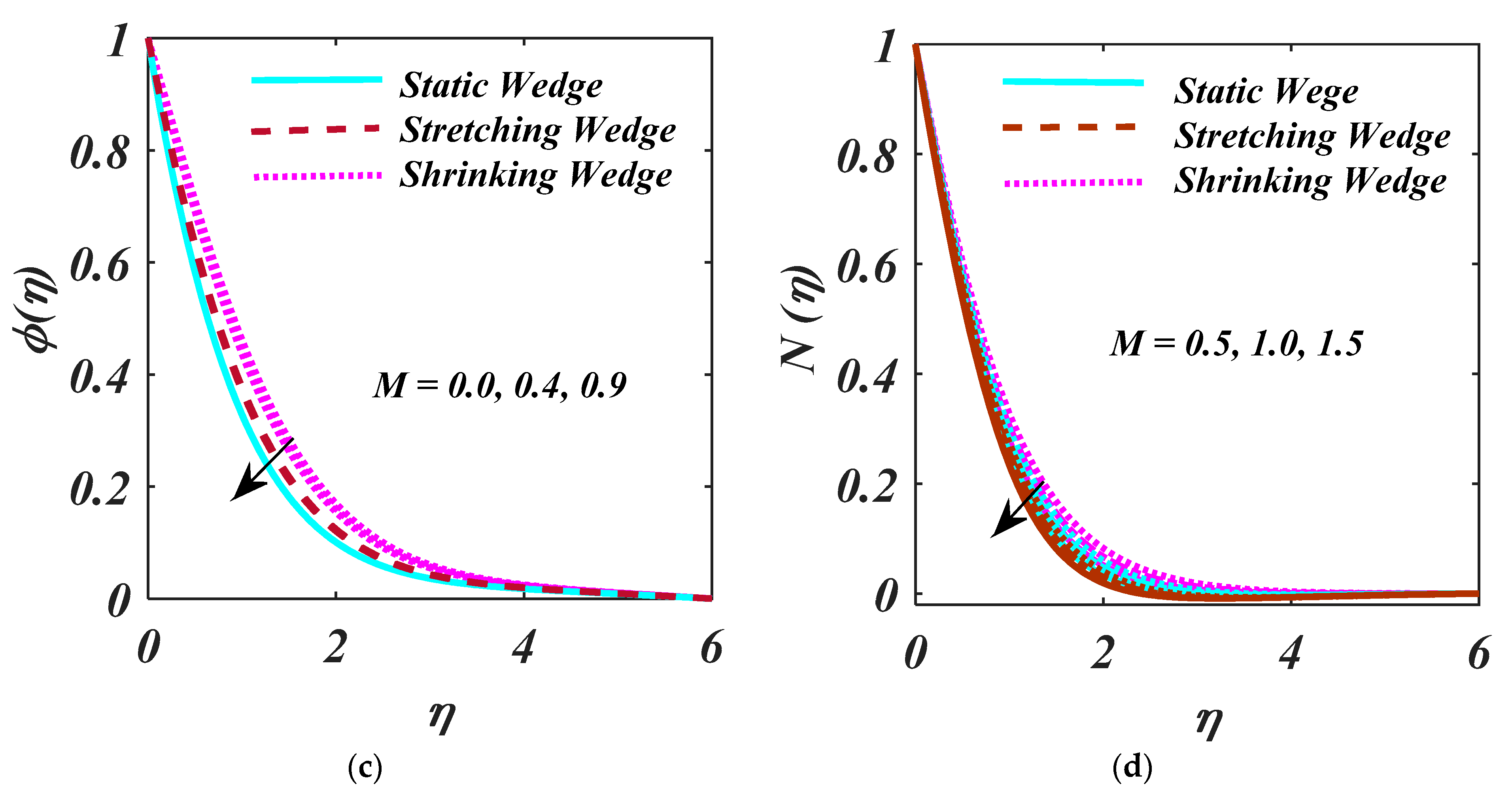
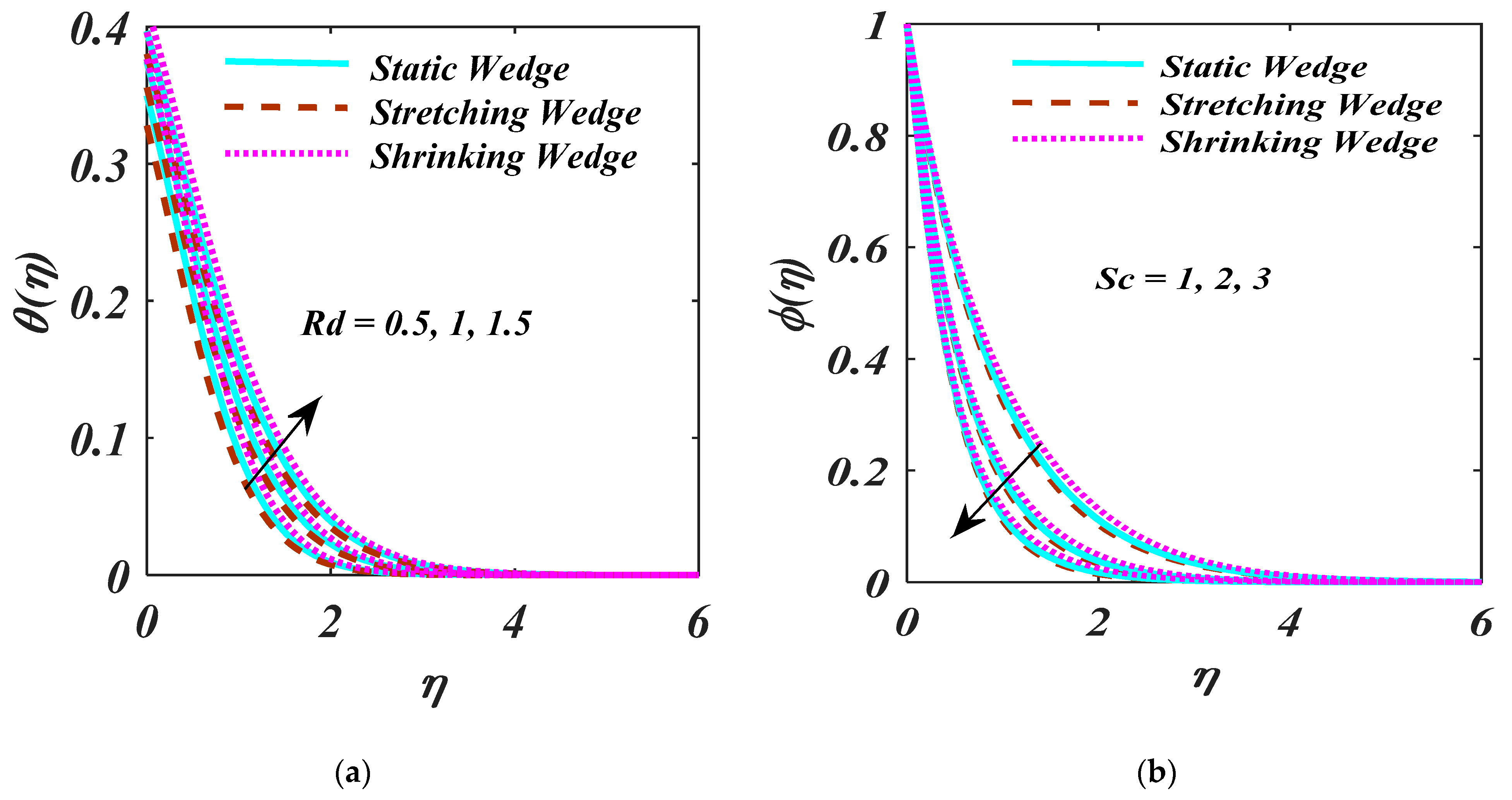
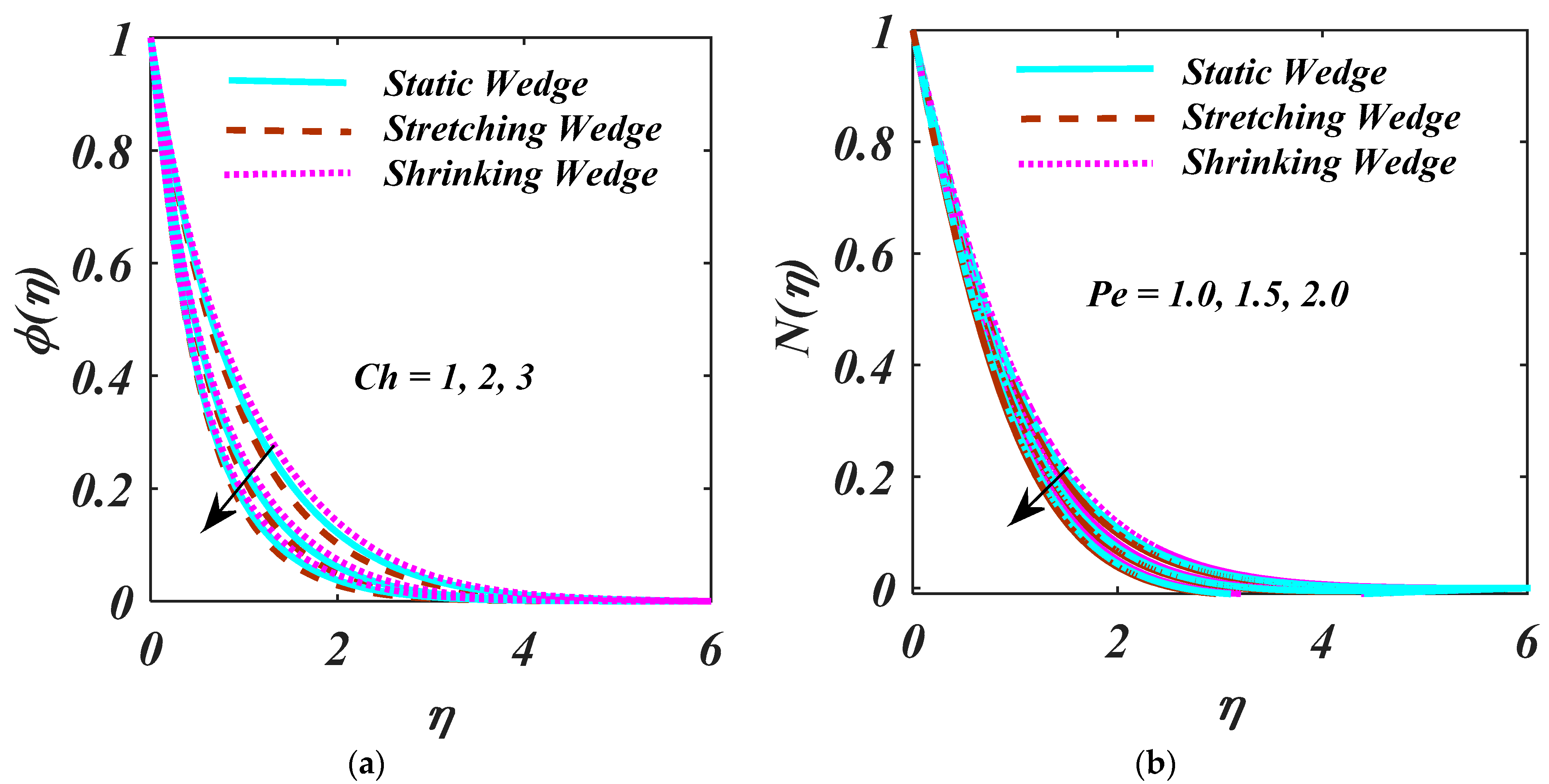
- An augmentation of leads to a reduction in the liquid concentration;
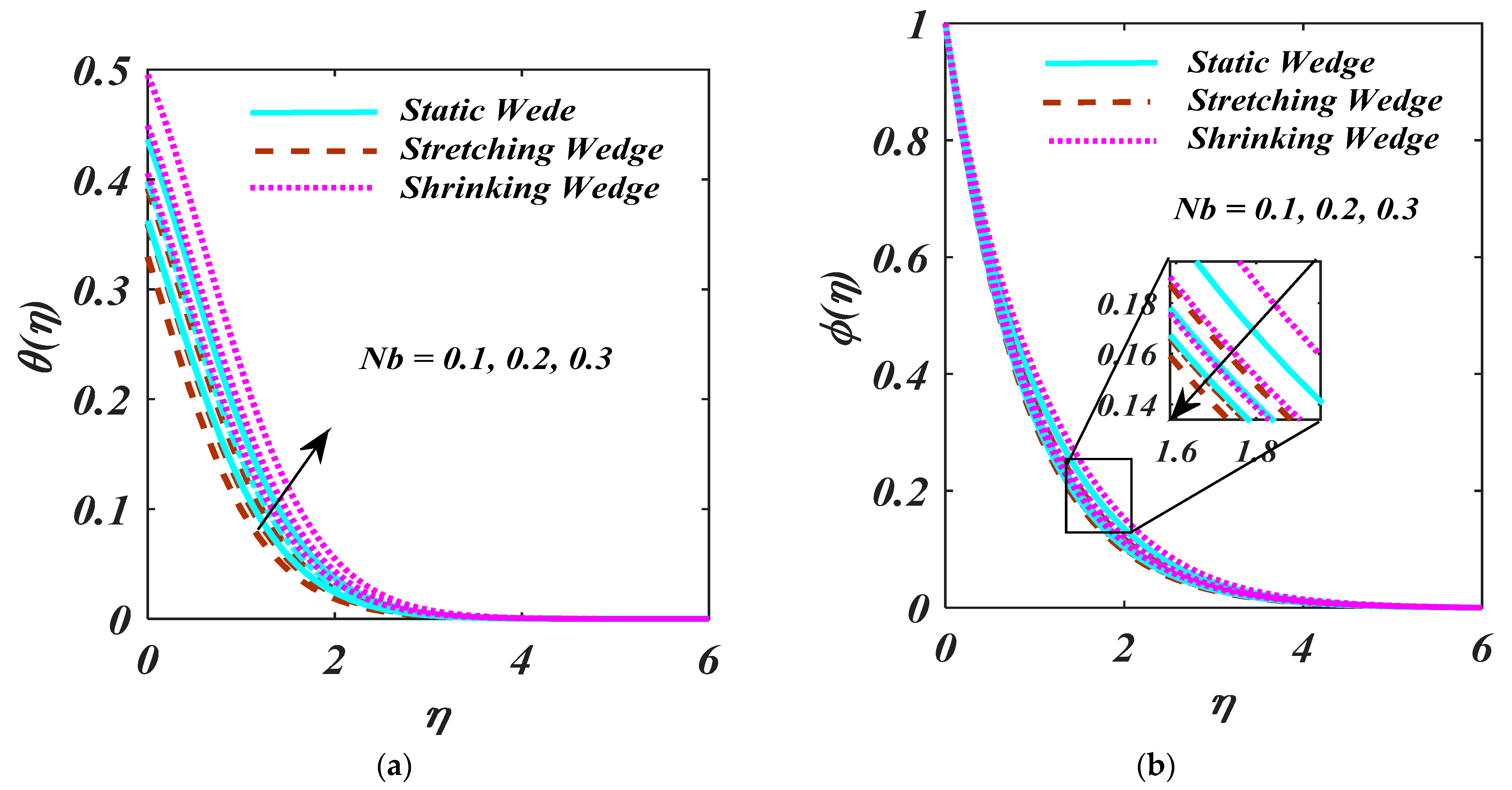
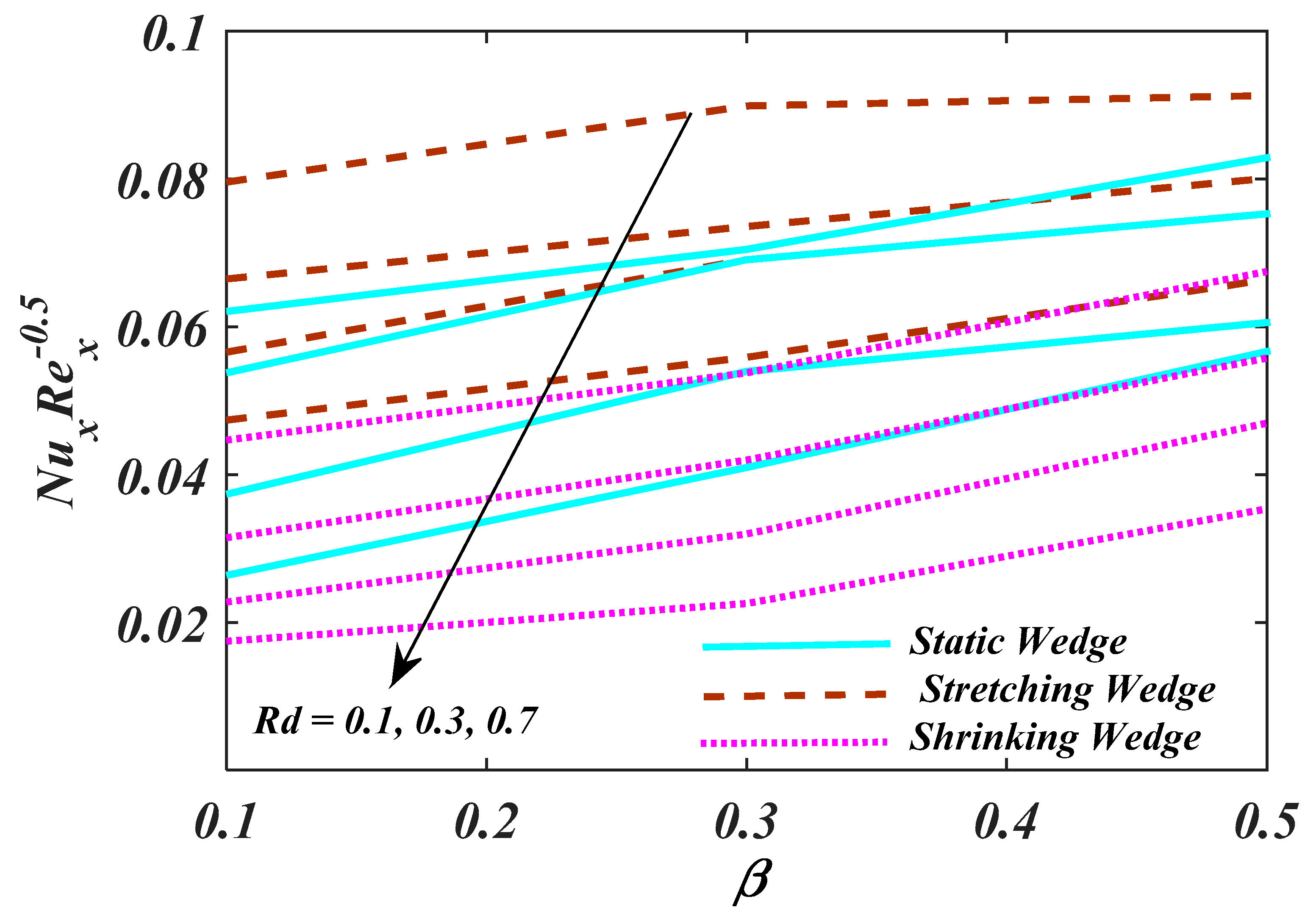
- Larger values of the Biot number show an increasing behaviour for temperature, but the opposite trend is noticed for the
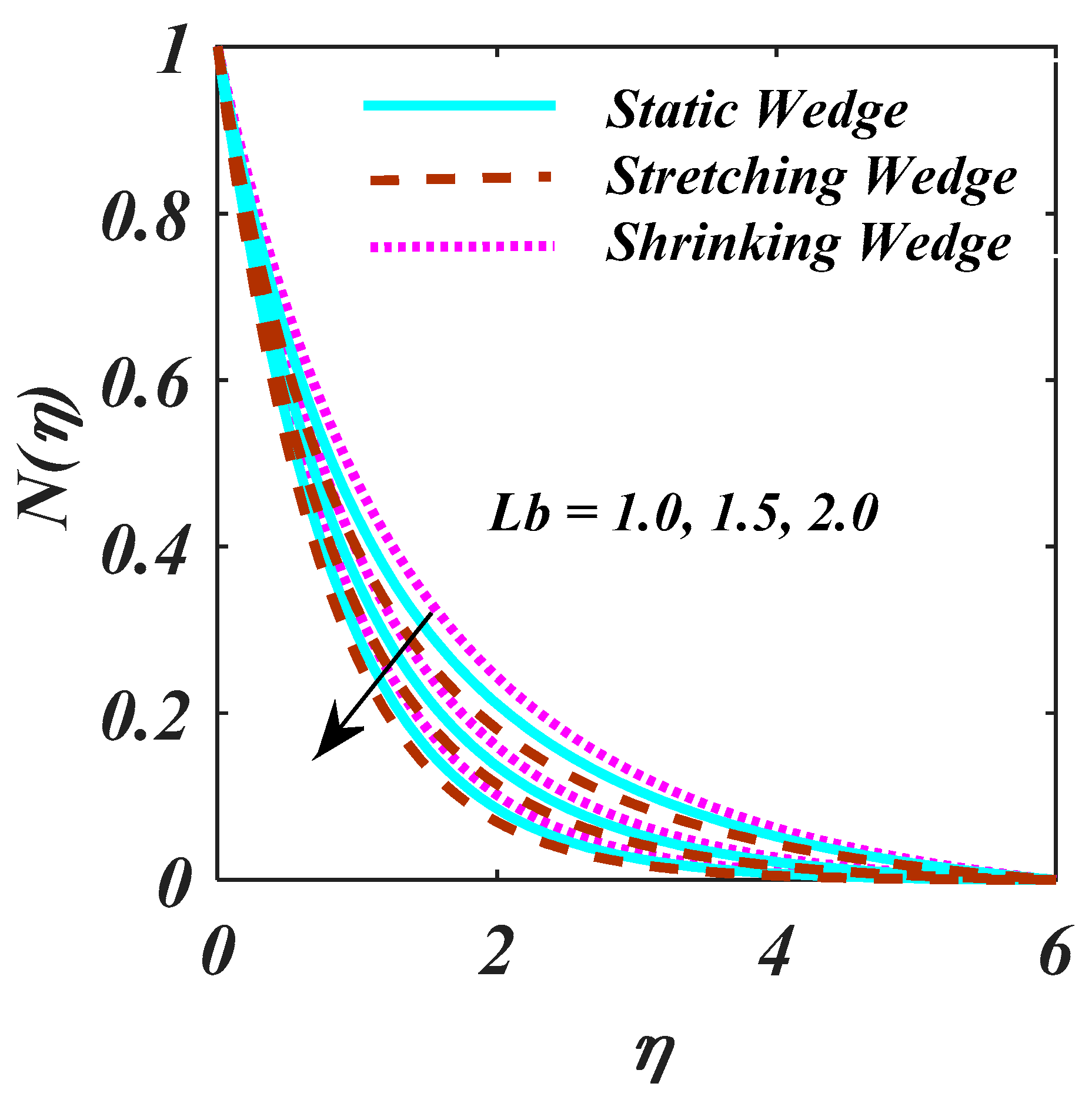
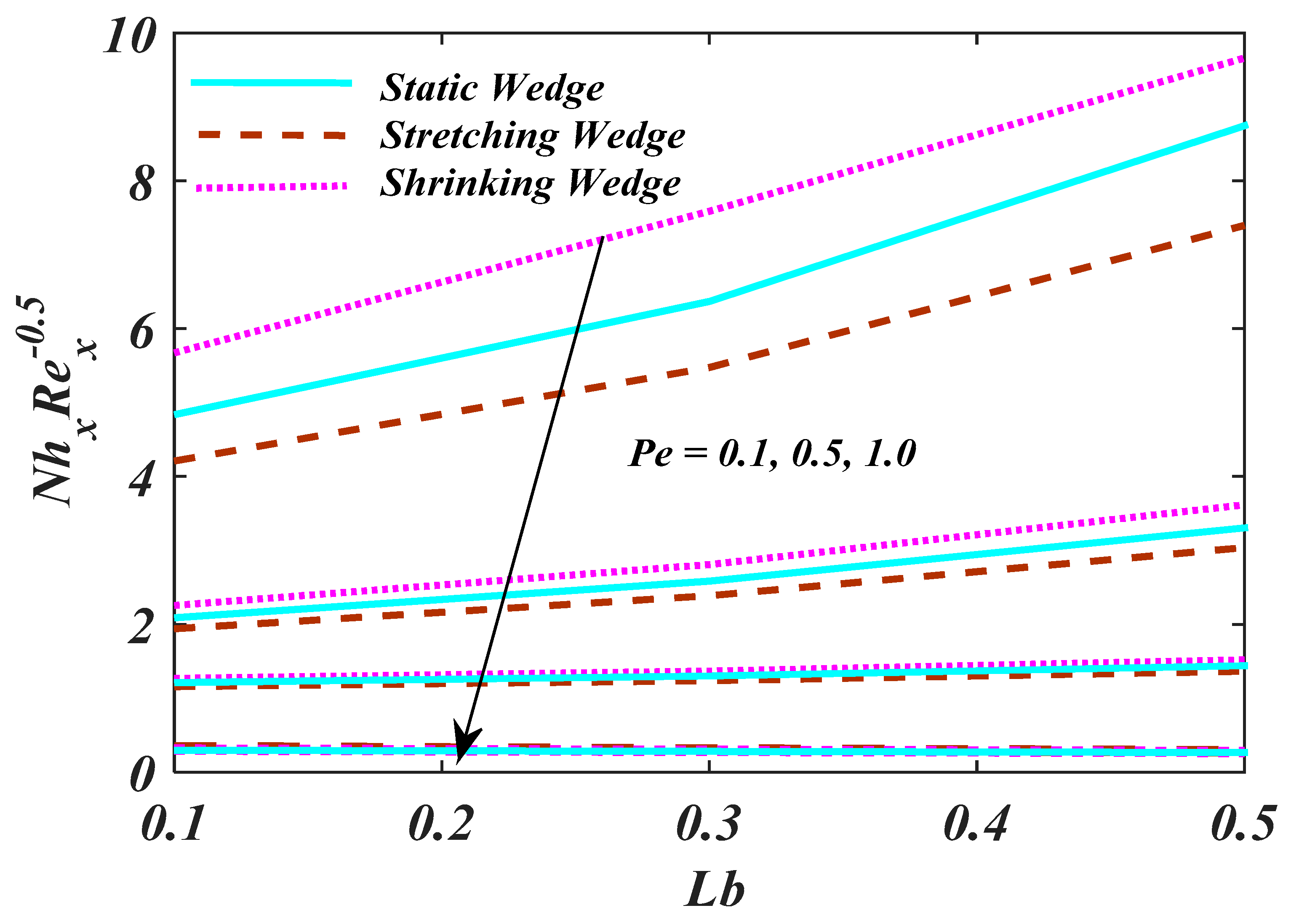
- By increasing the magnitude of the and , there is reduction behaviour.
- The density of the and the as the fluid parameters elevated, while the rate of the skin friction upsurges.
Author Contributions
Funding
Data Availability Statement
Conflicts of Interest
Nomenclature
| fluid variable | |
| fluid variable | |
| M | Magnetic variable |
| Unsteady variable | |
| velocity variable with ration | |
| Darcy Parameter | |
| K | Porosity variable |
| Pr | Prandtl number |
| Nt | Thermophoresis variable |
| Nb | Brownian motion |
| Pressure gradient parameter | |
| Bi | Biot number |
| Rd | Radiation parameter |
| Ch | Chemical reaction parameter |
| Sc | Schmidt number |
| Pe | Peclet number |
| Bioconvection Lewis number | |
| Temperature ratio parameter | |
| Skin fiction coefficient | |
| Heat transport coefficient (Nusselt) | |
| Mass Nusselt number | |
| motile density | |
| Similarity parameter | |
| Acceleration due to Gravity | |
| Velocity | |
| heat capacity with effectivness | |
| viscosity of Kinematic | |
| Stretching/shrinking variable | |
| Thermal diffusivity | |
| Mass diffusivity | |
| Thermophoresis diffusivity | |
| heat capacity of fluid | |
| Nanoparticles heat capacity | |
| Magnetic field strength | |
| Temperature of fluid | |
| Concentration susceptibility | |
| Variable temperature | |
| Variable concentration | |
| density of fluid | |
| Free stream velocity |
References
- Choi, S.U.S. Enhancing thermal conductivity of fluids with nanoparticles. Int. Mech. Eng. Cong. Exp. 1995, 66, 99–105. [Google Scholar]
- Buongiorno, J. Convective Transport in Nanofluids. J. Heat Transfer. 2006, 128, 240–250. [Google Scholar] [CrossRef]
- Bhatti, M.M.; Rashidi, M.M. Effects of thermo-diffusion and thermal radiation on Williamson nanofluid over a porous shrinking/stretching sheet. J. Mol. Liq. 2016, 221, 567–573. [Google Scholar] [CrossRef]
- Gireesha, B.J.; Gorla, R.S.R.; Mahanthesh, B. Effect of Suspended Nanoparticles on Three-Dimensional MHD Flow, Heat and Mass Transfer of Radiating Eyring-Powell Fluid Over a Stretching Sheet. J. Nanofluids 2015, 4, 474–484. [Google Scholar] [CrossRef]
- Ali, F.; Zaib, A. Unsteady flow of an Eyring-Powell nanofluid near stagnation point past a convectively heated stretching sheet. Arab J. Basic Appl. Sci. 2019, 26, 215–224. [Google Scholar] [CrossRef]
- Vaidya, H.; Prasad, K.V.; Vajravelu, K.; Shehzad, S.A.; Basha, H. Role of Variable Liquid Properties in 3D Flow of Maxwell Nanofluid Over Convectively Heated Surface: Optimal Solutions. J. Nanofluids 2019, 8, 1133–1146. [Google Scholar] [CrossRef]
- Kumar, K.A.; Sandeep, N.; Sugunamma, V.; Animasaun, I.L. Effect of irregular heat source/sink on the radiative thin film flow of MHD hybrid ferrofluid. J. Therm. Anal. Calorim. 2020, 139, 2145–2153. [Google Scholar] [CrossRef]
- Chamkha, A.J.; Mujtaba, M.; Quadri, A.; Issa, C. Thermal radiation effects on MHD forcedconvection flow adjacent to a non-isothermal wedge in the presence of a heat source or sink. Heat Mass Transf. 2003, 39, 305–312. [Google Scholar] [CrossRef]
- Sardar, H.; Khan, M.; Alghamdi, M. Multiple solutions for the modifiedFourier and Fick’s theories for Carreau nanofluid. Ind. J. Phys. 2020, 94, 1939–1947. [Google Scholar] [CrossRef]
- Danish, G.A.; Imran, M.; Tahir, M.; Waqas, H.; Asjad, M.I.; Akgül, A.; Baleanu, D. Effects of Non-Linear Thermal Radiation and Chemical Reaction on Time Dependent Flow of Williamson Nanofluid with Combine Electrical MHD and Activation Energy. J. Appl. Comput. Mech. 2021, 7, 546–558. [Google Scholar] [CrossRef]
- Ramesh, K.; Reddy, M.G.; Devakar, M. Biomechanical study of magneto hydrodynamic Prandtl nanofluid in a physiological vessel with thermal radiation and chemical reaction. Proc. I. Mech. E Part N J. Nanomater. Nanoeng. Nanosyst. 2018, 232, 95–108. [Google Scholar]
- Alwatban, A.M.; Khan, S.U.; Waqas, H.; Tlili, I. Interaction of Wu’s Slip Features in Bioconvection of Eyring Powell Nanoparticles with Activation Energy. Processes 2019, 7, 859. [Google Scholar] [CrossRef]
- Mekheimer, S.K.H.; Shaimaa Ramadan, F. New Insight into gyrotactic microorganisms for Bio-thermal convection of Prandtl nanofluid past a stretching/shrinking permeable sheet. SN Appl. Sci. 2020, 2, 450. [Google Scholar]
- Hussien, A.A.; Al-Kouz, W.; Yusop, N.; Abdullah, M.Z.; Janvekar, A.A. A Brief Survey of Preparation and Heat Transfer Enhancement of Hybrid Nanofluids. J. Mech. Eng. 2019, 65, 7–8. [Google Scholar] [CrossRef]
- Hussien, A.A.; Abdullah, M.Z.; Yusop, N.M.; Al-Kouz, W.; Mahmoudi, E.; Mehrali, M. Heat Transfer and Entropy Generation Abilities of MWCNTs/GNPs Hybrid Nanofluids in Microtubes. Entropy 2019, 21, 480. [Google Scholar] [CrossRef]
- Al-Kouz, W.; Swain, K.; Mahanthesh, B.; Jamshed, W. Significance of exponential space-based heat source and inclined magnetic field on heat transfer of hybrid nanoliquid with homogeneous–heterogeneous chemical reactions. Heat Transf. 2021, 50, 4086–4102. [Google Scholar] [CrossRef]
- Al-Kouz, W.; Medebber, M.A.; Elkotb, M.A.; Abderrahmane, A.; Aimad, K.; Al-Farhany, K.; Jamshed, W.; Moria, H.; Aldawi, F.; Saleel, C.A.; et al. Galerkin finite element analysis of Darcy–Brinkman–Forchheimer natural convective flow in conical annular enclosure with discrete heat sources. Energy Rep. 2021, 7, 6172–6181. [Google Scholar] [CrossRef]
- Mahanthesh, B.; Mackolil, J.; Radhika, M.; Al-Kouz, W. Significance of quadratic thermal radiation and quadratic convection on boundary layer two-phase flow of a dusty nanoliquid pasta vertical plate. Int. Commun. Heat Mass Transf. 2021, 120, 105029. [Google Scholar] [CrossRef]
- Al-Farhany, K.; Al-Dawody, M.F.; Hamzah, D.A.; Al-Kouz, W.; Said, Z. Numerical investigation of natural convection on Al2O3–water porous enclosure partially heated with two fins attached to its hot wall: Under the MHD effects. Appl. Nanosci. 2021, 1–18. [Google Scholar] [CrossRef]
- Al-Farhany, K.; Al-Chlaihawi, K.K.; Al-Dawody, M.F.; Biswas, N.; Chamkha, A.J. Effects of fins on magnetohydrodynamic conjugate natural convection in a nanofluid-saturated porous inclined enclosure. Int. Commun. Heat Mass Transf. 2021, 126, 105413. [Google Scholar] [CrossRef]
- Jamshed, W.; Al-Kouz, W.; Nasir, N.A.A.M. Computational single phase comparative study of inclined MHD in a Powell–Eyring nanofluid. Heat Transf. 2021, 50, 3879–3912. [Google Scholar] [CrossRef]
- Falkner, V.M.; Skan, S.W. Some approximate solutions of the boundary-layer equations. Philos. Mag. 1931, 7, 865–896. [Google Scholar] [CrossRef]
- Rajagopal, K.; Gupta, A.; Na, T. A note on the falkner-skan flows of a non-newtonian fluid. Int. J. Non-Linear Mech. 1983, 18, 313–320. [Google Scholar] [CrossRef]
- Lin, H.T.; Lin, L.K. Similarity solutions for laminar forced convection heat transfer fromwedges to fluids of any Prandtl number. Int. J. Heat Mass Transf. 1987, 30, 1111–1118. [Google Scholar] [CrossRef]
- Kuo, B.-L. Application of the differential transformation method to the solutions of Falkner-Skan wedge flow. Acta Mech. 2003, 164, 161–174. [Google Scholar] [CrossRef]
- Mishra, P.; Acharya, M.R.; Panda, S. Mixed convection MHD nanofluid flow over a wedge with temperature-dependent heat source. Pramana—J. Phys. 2021, 95, 52. [Google Scholar] [CrossRef]
- Ishak, A.; Nazar, R.; Pop, I. Moving wedge and flat plate in a micropolar fluid. Int. J. Eng. Sci. 2006, 44, 1225–1236. [Google Scholar] [CrossRef]
- Ganganapalli, S.; Kata, S.; Bhumarapu, V. Unsteady boundary layer flow of a Casson fluid past a wedge with wall slip velocity. J. Heat Mass Transf. Res. 2017, 4, 91–102. [Google Scholar]
- Raju, C.S.K.; Hoque, M.M.; Sivasankar, T. Radiative flow of Casson fluid over a movingwedge filled with gyrotactic microorganisms. Adv. Powder Technol. 2017, 28, 575–583. [Google Scholar] [CrossRef]
- Atif, S.; Hussain, S.; Sagheer, M. Heat and mass transfer analysis of time-dependent tangent hyperbolic nanofluid flow past a wedge. Phys. Lett. A 2019, 383, 1187–1198. [Google Scholar] [CrossRef]
- Khan, M.F.; Sulaiman, M.; Romero, C.A.T.; Alkhathlan, A. Falkner–Skan Flow with Stream-Wise Pressure Gradient and Transfer of Mass over a Dynamic Wall. Entropy 2021, 23, 1448. [Google Scholar] [CrossRef] [PubMed]
- Xu, H.; Pop, I. Fully developed mixed convection flow in a horizontal channel filled bya nanofluid containing both nanoparticles and gyrotactic microorganisms. Eur. J. Mech.-B/Fluids 2014, 1, 37–45. [Google Scholar] [CrossRef]
- Siddiqa, S.; Sulaiman, M.; Hossain, M.; Islam, S.; Gorla, R.S.R. Gyrotactic bioconvection flow of a nanofluid past a vertical wavy surface. Int. J. Therm. Sci. 2016, 108, 244–250. [Google Scholar] [CrossRef]
- Zuhra, S.; Khan, N.; Shah, Z.; Islam, S.; Bonyah, E. Simulation of bioconvection in the suspension of second grade nanofluid containing nanoparticles and gyrotactic microorganisms. AIP Adv. 2018, 8, 105210. [Google Scholar] [CrossRef]
- Mahdy, A. Unsteady Mixed Bioconvection Flow of Eyring–Powell Nanofluid with MotileGyrotactic Microorganisms Past Stretching Surface. BioNano Sci. 2021, 11, 295–305. [Google Scholar] [CrossRef]
- Xun, S.; Zhao, J.; Zheng, L.; Zhang, X. Bioconvection in rotating system immersed in nanofluid with temperature dependent viscosity and thermal conductivity. Int. J. Heat Mass Transf. 2017, 111, 1001–1006. [Google Scholar] [CrossRef]
- Alsaedi, A.; Khan, M.I.; Farooq, M.; Gull, N.; Hayat, T. Magnetohydrodynamic (MHD) stratified bioconvective flow of nanofluid due to gyrotactic microorganisms. Adv. Powder Technol. 2017, 28, 288–298. [Google Scholar] [CrossRef]
- Khan, N.A.; Alshammari, F.S.; Romero, C.A.T.; Sulaiman, M.; Mirjalili, S. An Optimistic Solver for the Mathematical Model of the Flow of Johnson Segalman Fluid on the Surface of an Infinitely Long Vertical Cylinder. Materials 2021, 14, 7798. [Google Scholar] [CrossRef]
- Zhang, Y.; Rong, Q. High-Efficiency Drive for IPMSM Based on Model Predictive Control. In Proceedings of the 2021 24th International Conference on Electrical Machines and Systems (ICEMS), Gyeongju, Korea, 31 October–3 November 2021; pp. 588–592. [Google Scholar]
- Khan, N.A.; Sulaiman, M.; Romero, C.A.T.; Alarfaj, F.K. Numerical Analysis of Electrohydrodynamic Flow in a Circular Cylindrical Conduit by Using Neuro Evolutionary Technique. Energies 2021, 14, 7774. [Google Scholar] [CrossRef]
- Powell, R.E.; Eyring, H. Mechanisms for the Relaxation Theory of Viscosity. Nature 1944, 154, 427–428. [Google Scholar] [CrossRef]
- Gholinia, M.; Hosseinzadeh, K.; Mehrzadi, H.; Ganji, D.; Ranjbar, A. Investigation of MHD Eyring–Powell fluid flow over a rotating disk under effect of homogeneous–heterogeneous reactions. Case Stud. Therm. Eng. 2019, 13, 100356. [Google Scholar] [CrossRef]
- Khan, S.U.; Nasir, A.; Zaheer, A. Influence of Heat Generation/Absorption with Convective Heat and Mass Conditions in Unsteady Flow of Eyring Powell Nanofluid Over Porous Oscillatory Stretching Surface. J. Nanofluids 2016, 5, 351–362. [Google Scholar] [CrossRef]
- Salawu, S.; Ogunseye, H. Entropy generation of a radiative hydromagnetic Powell-Eyring chemical reaction nanofluid with variable conductivity and electric field loading. Results Eng. 2020, 5, 100072. [Google Scholar] [CrossRef]
- Abegunrin, O.; Animasaun, I.; Sandeep, N. Insight into the boundary layer flow of non-Newtonian Eyring-Powell fluid due to catalytic surface reaction on an upper horizontal surface of a paraboloid of revolution. Alex. Eng. J. 2018, 57, 2051–2060. [Google Scholar] [CrossRef]
- Rahimi, J.; Ganji, D.; Khaki, M.; Hosseinzadeh, K. Solution of the boundary layer flow of an Eyring-Powell non-Newtonian fluid over a linear stretching sheet by collocation method. Alex. Eng. J. 2017, 56, 621–627. [Google Scholar] [CrossRef]
- Reddy, S.R.R.; Reddy, B.A.; Bhattacharyya, K. Effect of nonlinearthermal radiation on 3D magneto slip flow of Eyring-Powell nanofluidflow over a slendering sheet with binary chemical reaction andarrhenius activation energy. Adv. Powder Technol. 2019, 30, 3203–3213. [Google Scholar] [CrossRef]
- Khan, M.; Azam, M.; Munir, A. On unsteady Falkner-Skan flow of MHD Carreau nanofluid past a static/moving wedge with convective surface condition. J. Mol. Liq. 2017, 230, 48–58. [Google Scholar] [CrossRef]
- Abbasi, A.; Farooq, W.; Tag-ElDin, E.S.M.; Khan, S.U.; Khan, M.I.; Guedri, K.; Elattar, S.; Waqas, M.; Galal, A.M. Heat Transport Exploration for Hybrid Nanoparticle (Cu, Fe3O4)-Based Blood Flow via Tapered Complex Wavy Curved Channel with Slip Features. Micromachines 2022, 13, 1415. [Google Scholar] [CrossRef] [PubMed]


| Khan et al. [48] | Current Outcomes | % Error | |
|---|---|---|---|
| 0.0 | 0.4696005 | 0.4695999 | |
| 0.1 | 0.5870353 | 0.5870352 | |
| 0.3 | 0.7747546 | 0.7747545 | |
| 0.5 | 0.9276800 | 0.9276799 | |
| 1.0 | 1.2325880 | 1.2325876 |
| 0.1 | 0.1 | 0.1 | 0.3 | 0.1 | 0.1 | 0.1 | 0.2637 | 1.5630 | 1.2408 |
| 0.5 | 1.4654 | 1.8936 | 1.3256 | ||||||
| 1.0 | 1.7553 | 1.9796 | 1.6211 | ||||||
| 0.1 | 0.2 | 0.4 | 0.3 | 0.3 | 0.2 | 0.3 | 1.7534 | 1.8921 | 1.9061 |
| 0.5 | 2.1194 | 2.2681 | 2.3521 | ||||||
| 1.0 | 2.5818 | 2.7586 | 2.8408 | ||||||
| 0.1 | 0.3 | 0.7 | 0.3 | 0.6 | 0.3 | 0.6 | 2.2342 | 2.0140 | 2.2460 |
| 0.5 | 2.6377 | 2.5138 | 2.5436 | ||||||
| 1.0 | 2.9625 | 2.9398 | 2.8549 | ||||||
| 0.1 | 0.4 | 0.9 | 0.3 | 0.9 | 0.4 | 0.9 | 2.4091 | 2.1823 | 2.3869 |
| 0.5 | 2.7604 | 2.7382 | 2.6117 | ||||||
| 1.0 | 3.1190 | 3.7998 | 2.9589 |
λ = 1 | λ = − 2.5 | λ = 2.5 | ||||||
|---|---|---|---|---|---|---|---|---|
| 0.1 | 0.1 | 0.3 | 0.6 | 1.0 | 0.4 | 0.0447 | 0.0621 | 0.0796 |
| 0.3 | 0.0538 | 0.0705 | 0.0899 | |||||
| 0.7 | 0.0675 | 0.0829 | 0.0913 | |||||
| 0.1 | 0.2 | 0.5 | 0.8 | 2.0 | 0.6 | 0.0358 | 0.0538 | 0.0665 |
| 0.3 | 0.0420 | 0.0691 | 0.0736 | |||||
| 0.7 | 0.0558 | 0.0753 | 0.0801 | |||||
| 0.1 | 0.3 | 0.7 | 1.0 | 3.0 | 0.8 | 0.0228 | 0.0374 | 0.0566 |
| 0.3 | 0.0320 | 0.0540 | 0.0691 | |||||
| 0.7 | 0.0470 | 0.0606 | 0.0753 | |||||
| 0.1 | 0.4 | 0.9 | 1.2 | 4.0 | 1.0 | 0.0176 | 0.0264 | 0.0474 |
| 0.3 | 0.0226 | 0.0410 | 0.0559 | |||||
| 0.7 | 0.0354 | 0.0567 | 0.0664 |
| 0.1 | 0.1 | 0.5 | 0.4 | 0.2 | 0.4 | 1.0284 | 0.9785 | 1.0747 |
| 0.5 | 0.9567 | 0.9057 | 1.0037 | |||||
| 1.0 | 0.8763 | 0.8241 | 0.9241 | |||||
| 0.1 | 0.3 | 1.0 | 0.6 | 0.4 | 0.6 | 1.2502 | 1.1948 | 1.3017 |
| 0.5 | 1.1428 | 1.0846 | 1.1963 | |||||
| 1.0 | 1.0292 | 0.9682 | 1.0846 | |||||
| 0.1 | 0.4 | 1.5 | 0.8 | 0.6 | 0.8 | 1.2788 | 1.2286 | 1.3259 |
| 0.5 | 1.1658 | 1.1175 | 1.2233 | |||||
| 1.0 | 1.0630 | 1.0029 | 1.1167 | |||||
| 0.1 | 0.6 | 2.0 | 1.0 | 0.8 | 1.0 | 1.2932 | 1.1849 | 1.3304 |
| 0.5 | 1.2017 | 1.1571 | 1.1603 | |||||
| 1.0 | 1.1095 | 1.0573 | 1.1557 |
| 0.1 | 0.5 | 0.2 | 0.1 | 0.4 | 0.2970 | 0.3054 | 0.3381 |
| 0.5 | 0.2804 | 0.2886 | 0.3073 | ||||
| 1.0 | 0.2653 | 0.2734 | 0.2734 | ||||
| 0.1 | 1.0 | 0.6 | 0.3 | 0.6 | 1.2121 | 1.2694 | 1.1572 |
| 0.5 | 1.3011 | 1.3679 | 1.2378 | ||||
| 1.0 | 1.4400 | 1.5206 | 1.3649 | ||||
| 0.1 | 1.5 | 1.0 | 0.6 | 0.8 | 2.0884 | 2.2555 | 1.9393 |
| 0.5 | 2.5836 | 2.8085 | 2.3871 | ||||
| 1.0 | 3..3051 | 3.6163 | 3.0382 | ||||
| 0.1 | 2.0 | 1.4 | 0.9 | 1.0 | 4.8372 | 5.6726 | 4.2083 |
| 0.5 | 6.3681 | 7.5882 | 5.4749 | ||||
| 1.0 | 8.7454 | 9.6614 | 7.3976 |
Publisher’s Note: MDPI stays neutral with regard to jurisdictional claims in published maps and institutional affiliations. |
© 2022 by the authors. Licensee MDPI, Basel, Switzerland. This article is an open access article distributed under the terms and conditions of the Creative Commons Attribution (CC BY) license (https://creativecommons.org/licenses/by/4.0/).
Share and Cite
Ahmed, M.F.; Zaib, A.; Ali, F.; Bafakeeh, O.T.; Tag-ElDin, E.S.M.; Guedri, K.; Elattar, S.; Khan, M.I. Numerical Computation for Gyrotactic Microorganisms in MHD Radiative Eyring–Powell Nanomaterial Flow by a Static/Moving Wedge with Darcy–Forchheimer Relation. Micromachines 2022, 13, 1768. https://doi.org/10.3390/mi13101768
Ahmed MF, Zaib A, Ali F, Bafakeeh OT, Tag-ElDin ESM, Guedri K, Elattar S, Khan MI. Numerical Computation for Gyrotactic Microorganisms in MHD Radiative Eyring–Powell Nanomaterial Flow by a Static/Moving Wedge with Darcy–Forchheimer Relation. Micromachines. 2022; 13(10):1768. https://doi.org/10.3390/mi13101768
Chicago/Turabian StyleAhmed, Muhammad Faizan, A. Zaib, Farhan Ali, Omar T. Bafakeeh, El Sayed Mohamed Tag-ElDin, Kamel Guedri, Samia Elattar, and Muhammad Ijaz Khan. 2022. "Numerical Computation for Gyrotactic Microorganisms in MHD Radiative Eyring–Powell Nanomaterial Flow by a Static/Moving Wedge with Darcy–Forchheimer Relation" Micromachines 13, no. 10: 1768. https://doi.org/10.3390/mi13101768
APA StyleAhmed, M. F., Zaib, A., Ali, F., Bafakeeh, O. T., Tag-ElDin, E. S. M., Guedri, K., Elattar, S., & Khan, M. I. (2022). Numerical Computation for Gyrotactic Microorganisms in MHD Radiative Eyring–Powell Nanomaterial Flow by a Static/Moving Wedge with Darcy–Forchheimer Relation. Micromachines, 13(10), 1768. https://doi.org/10.3390/mi13101768