1. Introduction
The Internet of Things (IoT), which excludes PCs, tablets and smartphones, will grow to 25 billion units installed in 2021, representing an almost 30-fold increase from 0.9 billion in 2009 [
1]. Additionally, more and more IoT systems are working in battery-powered scenarios or even battery-less scenarios [
2,
3]. Given the limitation of energy supply and the demand for performance, system designers are paying more attention to power consumption, especially for the embedded processor which is one of the core components in IoT systems [
4,
5]. Due to its responsibility for data computation and system control, an embedded processor has to deal with a variety of complicated tasks with different workloads, making it difficult to balance peak performance and power consumption for various scenarios. Improving energy efficiency is now becoming a key concern for all designers [
6,
7].
To satisfy the performance and power demands of diverse embedded systems, processors with different micro-architectures are employed in different devices. For commercial use, ARM Ltd. has introduced Cortex-M series processors, including Cortex-M0, Cortex-M3, etc. [
8]. These processors are designed for deterministic, real-time embedded processing and microcontroller applications, and are optimized for low-cost and energy-efficiency. In addition to processors in industry, many cores are implemented in academia [
9,
10,
11,
12,
13,
14]. For example, the Pulp team from ETH and the University of Bologna has proposed several processors, including Zero-riscy, Riscy, and Ariane. All these cores are implemented elaborately for different scenarios, and are silicon-proven for commercial use rather than research-use-only [
15,
16,
17,
18,
19].
In many embedded systems, peak performance is a key factor for the processor selection. However, more complex architectures provide better performance and worse power consumption. Despite finishing an instruction in a shorter time, a high-performance processor will still dissipate more energy on the same task and consume more power in idle state.
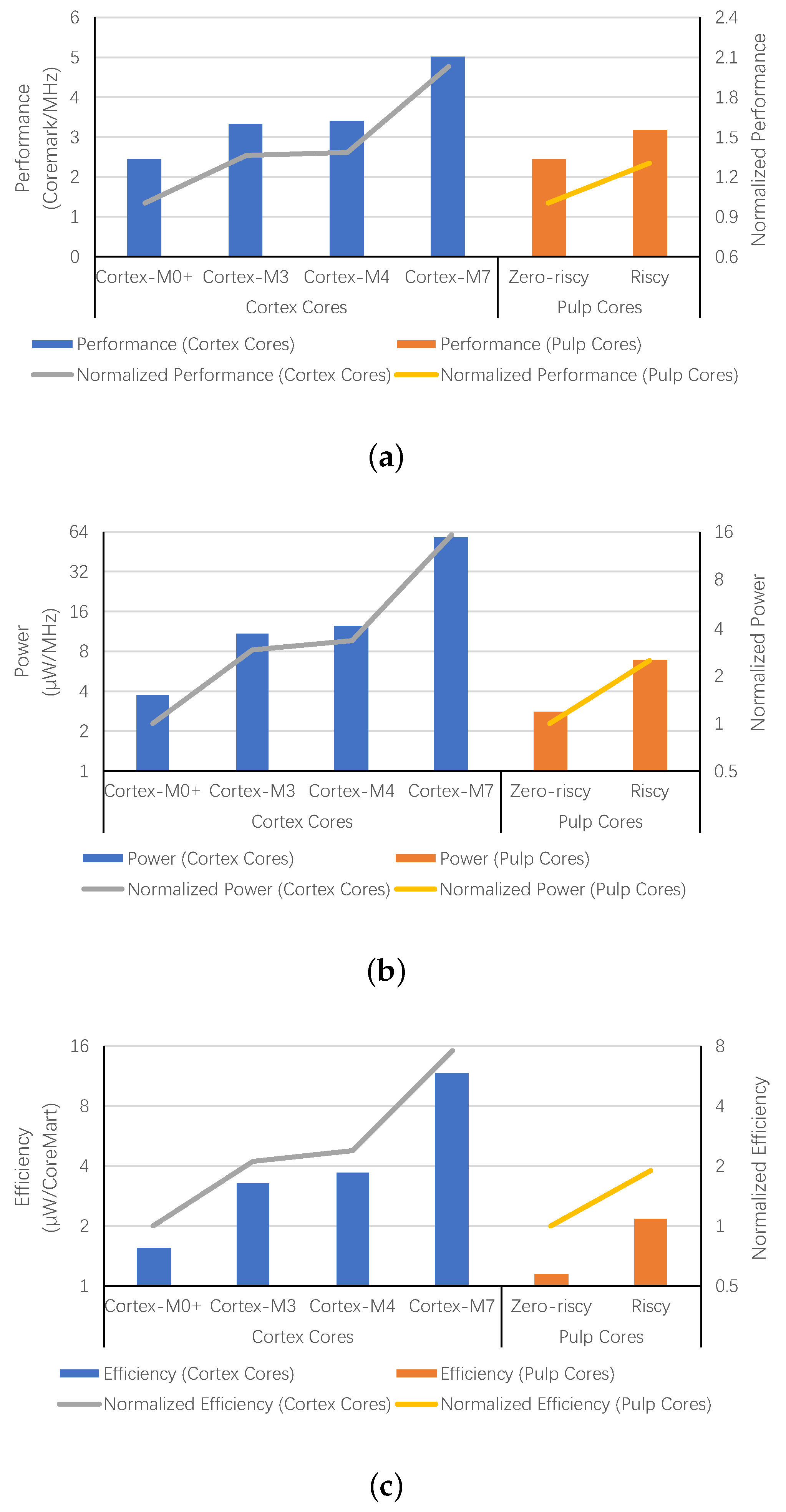
Figure 1 demonstrates the performance, power consumption and energy efficiency of different embedded cores. The performance of Cortex-M3, shown in
Figure 1a, is 1.36 times that of Cortex-M0+ [
20,
21]. However, it consumes 2.89 times the power, which is demonstrated in
Figure 1b. According to the results shown in
Figure 1c, the tremendous power increase leads to 113% more energy dissipation to execute the CoreMark benchmark once. As the performance and power increase, the energy efficiency for Cortex-M4 and Cortex-M7 is even worse [
22,
23]. Compared to Cortex-M0+, they use 138% and 656% more energy for the same task. Besides the Cortex-M series cores, Pulp cores are also evaluated in
Figure 1. The performance of Riscy is better than Zero-riscy. However, Zero-riscy consumes less energy for a task due to its simpler micro-architecture. For power reduction, scaling down the supply voltage is the most widely used method [
24,
25]. Some processors are designed to work at a low voltage, or even work at near-threshold or sub-threshold voltage. However, the voltage scaling has slowed down in recent years, since it is no longer possible to scale the threshold voltage because of rising leakage currents [
26]. Thus, architecture optimization is now necessary to improve energy efficiency further.
The main focus of this paper is designing an embedded processor with variable architecture. The variable core could change its pipeline structure and shut down the branch predictor to reduce power consumption. The main contributions of this paper are as follows:
We present a detailed analysis of the energy distribution of different embedded processors and point out the inefficiency in a processor based on four baseline cores with state-of-the-art performance and power efficiency.
We propose a variable processor which could work with different micro-architectures in different working modes.
We present a software-based mode switching method that simplifies the circuit design and reduces the hardware overhead.
We show the possibility to improve the energy efficiency of an embedded processor by adding simple bypass data paths for architecture switching.
The rest of this paper is structured as follows: Related works are discussed in
Section 2.
Section 3 presents the baseline processors and analyzes the power distribution in these processors.
Section 4 introduces the hardware architecture and software interface of the variable processor. Results and evaluations are shown in
Section 5.
Section 6 concludes this paper.
2. Related Work
In many cases, processors only work on compute-intensive tasks for short periods of time, and on low-load tasks most of the time. To improve the energy efficiency, numerous studies are presented for performance and power consideration [
27,
28,
29,
30]. Both circuit-level and architecture-level optimizations were involved in these studies. According to their methods, all the designs can be categorized into (1) systems with dynamic voltage and frequency scaling, (2) heterogeneous multi-core processors and (3) fine-grained heterogeneous processors.
2.1. Dynamic Voltage and Frequency Scaling (DVFS)
The voltage of the power supply has a significant impact on energy dissipation. Many digital systems are designed based on a low voltage supply for power reduction. However, a fixed low voltage of the power supply is harmful to the peak performance. To improve energy efficiency and meet the performance demand, dynamic voltage and frequency scaling (DVFS) is widely used, especially for IoT systems [
31,
32]. By regulating the supply voltage and clock frequency dynamically, a system could manage its performance and power according to the working status. As one of the core components in digital systems, processors benefit greatly from DVFS in low-load conditions as well [
33,
34]. Besides, DVFS could easily be incorporated into a processor with architecture-level optimization. However, the voltage scaling has slowed down in recent years, since it became impossible to scale the threshold voltage because of rising leakage currents [
26]. Considering the limitations of voltage scaling, the utility of DVFS has been decreasing, making it difficult to reduce power dissipation further without architecture optimization.
2.2. Heterogeneous Multi-Core Processors
Many works have focused on exploring heterogeneity in a digital system to improve efficiency. Annavaram et al. proposed to use small cores for parallel tasks, while serial tasks are run on a big core [
35]. Considering the power limitation, it will improve the overall energy efficiency. Kumar et al. advocated assigning tasks to different cores with various power and performance characteristics, so that each core could achieve the best power efficiency [
28,
29]. Besides the asymmetric multicore processors, ARM Ltd. has proposed big.LITTLE technology, which contains a big core (Cortex-A15) and a little core (Cortex-A7) in a cluster and only activates one core at a time. Thread switches between cores in coarse granularity. For the same task, the energy efficiency of little cores is much better than that of big cores [
36]. To further improve the execution efficiency of these processors, many studies about task mapping and thread switching were also conducted [
37,
38,
39].
2.3. Fine-Grained Heterogeneous Processors
Heterogeneous multi-core processors improve performance within a limited power budget, but also lead to additional costs. To avoid the significant drawbacks in terms of area and latency, researchers suggested achieving heterogeneity within a single core. Andrew Lukefahr et al. proposed a composite core with a big
Engine and a small
Engine. The two
Engines share an L1-cache, a branch predictor and an architectural register file. In the composite core, thread switching is controlled dynamically by an online controller [
40]. Sudarshan Srinivasan et al. designed a processor that could work in different modes with different micro-architecture resources, e.g., fetch width, issue width and buffer sizes. The processor will perform a program in an appropriate mode determined by a runtime mechanism and switch to another mode when the workload has been changed [
41].
Previous works focused on complex heterogeneous processors using an Out-of-Order core as the big core. However, they are too heavy to work in ultra-low-power scenarios. Considering the power limitation, in-order cores without multiple issue ports are always preferred.
3. Power Consumption in Embedded Processors
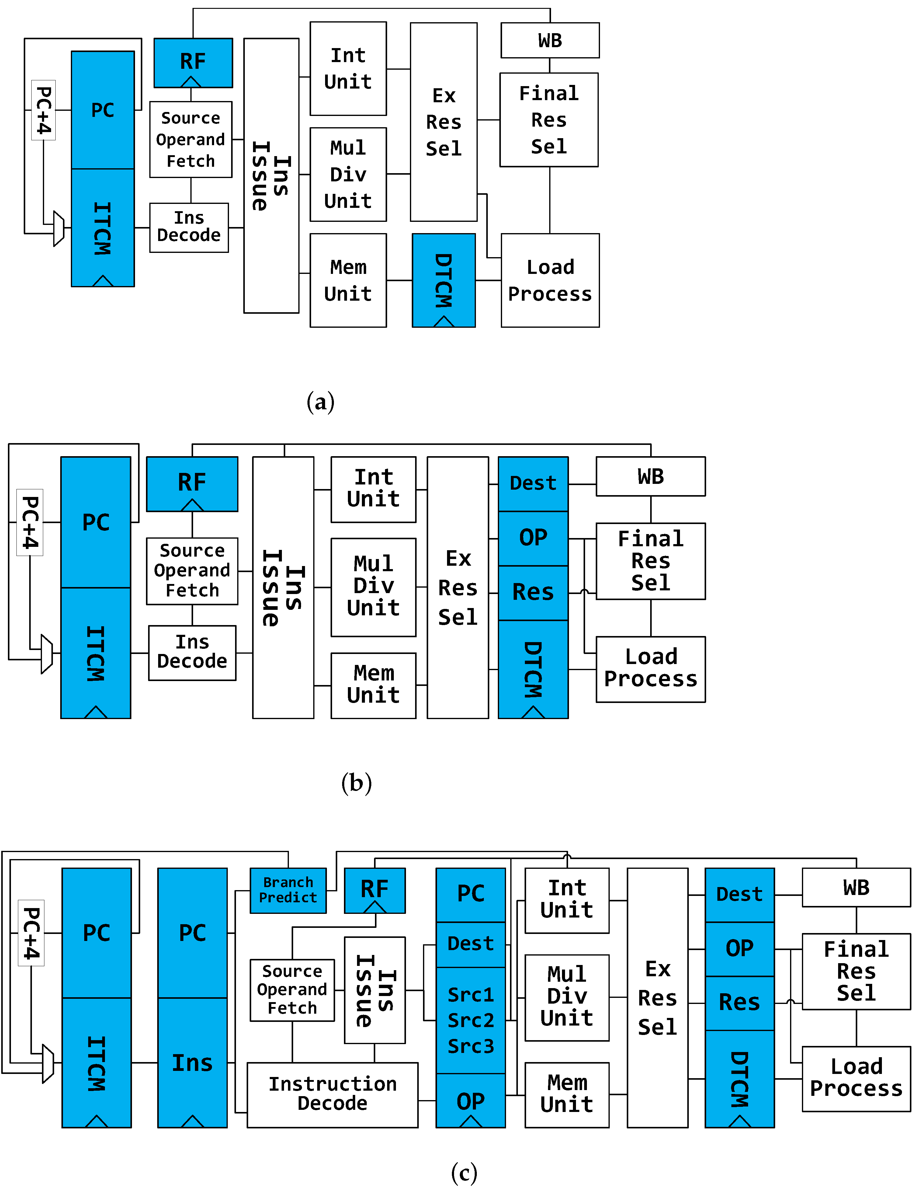
Analyzing the power impact of each part in processors makes sense in order to identify the inefficient units in idle state. To explore the power distribution, we have designed four RISC-V cores supporting RVC32IM and found out the main contributor to energy dissipation. Instructions and data are stored in separate SRAMs. All decoding and execution units are the same in these processors. Thus, the distinction in energy efficiency is mainly caused by different structures, such as control units, branch predictors, pipeline stages, etc. These processors were designed in three different pipeline structures:
TinyCore. The most simplified architecture is employed in this core. As is shown in
Figure 2a, there is no pipeline register in TinyCore. Only load, multiplication and division instructions can cause stalls in this processor.
LittleCore. It has pipeline registers before the Write-Back unit.
Figure 2b demonstrates its architecture. Only multi-cycle instructions will stall this processor.
PipeCore. The other two processors have the same architecture as the PipeCore shown in
Figure 2c. They are both single-issue in-order cores with four pipeline stages and a branch predictor. The only difference between them is the branch prediction algorithm.
Always-Not-Taken and Gshare are used, respectively, in PipeCoreA and PipeCoreG. Gshare is only a tiny predictor without branch target buffer (BTB) and return address stack (RAS) due to their huge requirements in terms of area and energy consumption. Thus, all branch predictions are completed in Decode, which can get the branch target from the instruction. The Gshare predictor has 256 entries. That number of entries was selected because of its better balance between performance and energy efficiency. The maximum frequencies of the cores are 290 MHz (TinyCore), 310 MHz (LittleCore), 740 MHz (PipeCoreA) and 720 MHz (PipeCoreG).
The area, performance and power consumption of these baseline processors are shown in
Table 1. All features are close to those of the state-of-the-art cores in academia and industry [
8,
42]. To further explore the energy efficiency and power distribution of different cores, we have synthesized all these processors with UMC 40LP technology, and evaluated the performance and energy efficiency with the trace of 17 benchmarks in Embench [
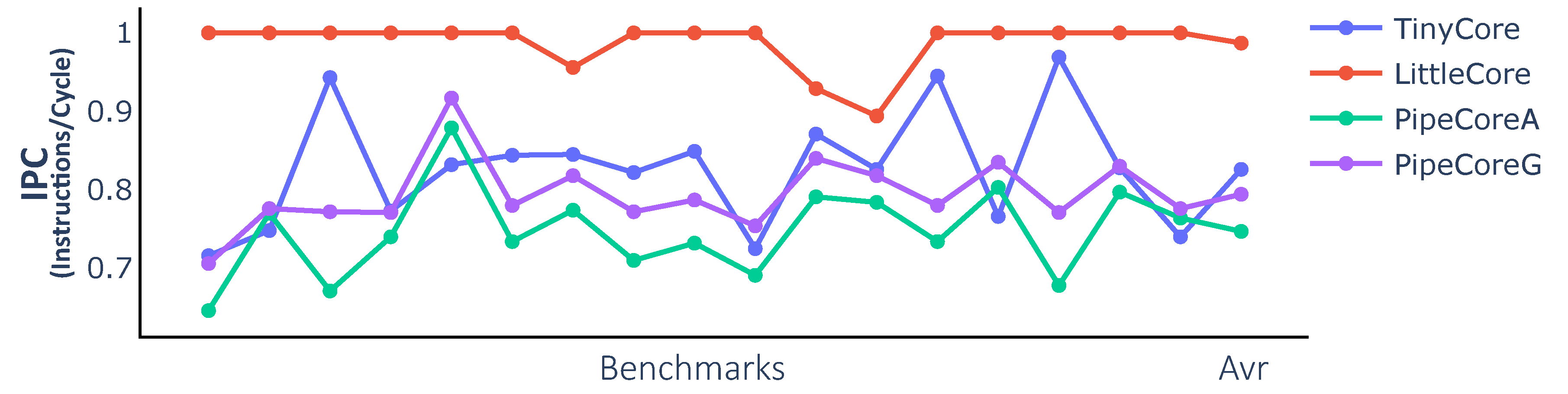
43]. All cores were synthesized with relaxed timing constraints and run at the frequency of 20 MHz. The execution efficiency of each core was evaluated by the number of instructions per cycle (IPC).
As shown in
Figure 3, there are wide variations in execution efficiency. The IPC values of PipeCores are lower than those of TinyCore and LittleCore. This reduction is caused by the more complex pipeline structure, leading to additional speculative execution and data hazard stalls in the processor. The IPC of PipeCoreG is better than PipeCoreA because of the Gshare predictor. LittleCore has a better IPC than TinyCore, since all load-conflicts are avoided by splitting the load operation into two different pipeline stages and forwarding the result before writing back. Considering the maximum frequency, PipeCoreG offers the best performance followed by PipeCoreA, LittleCore and TinyCore.
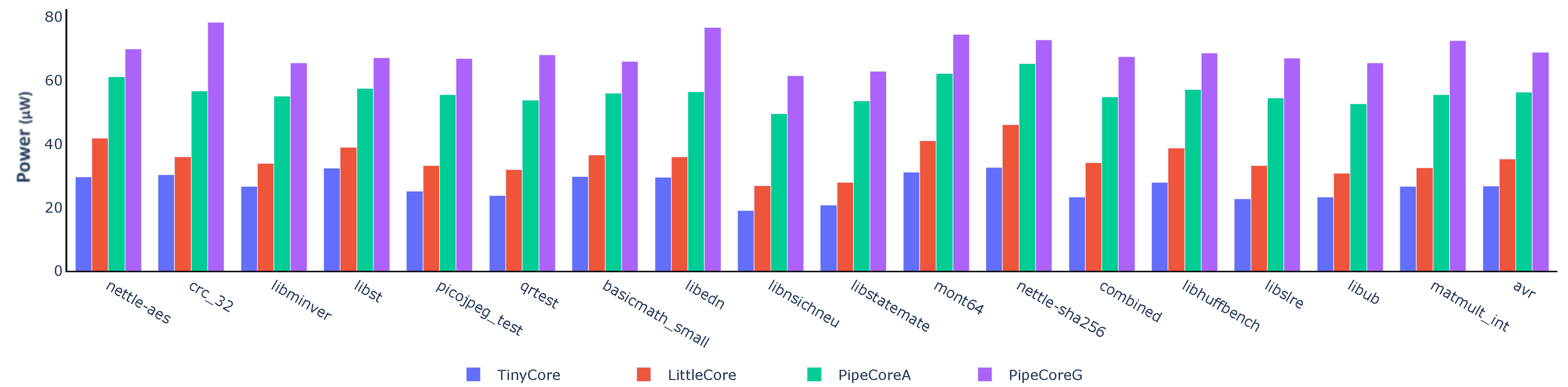
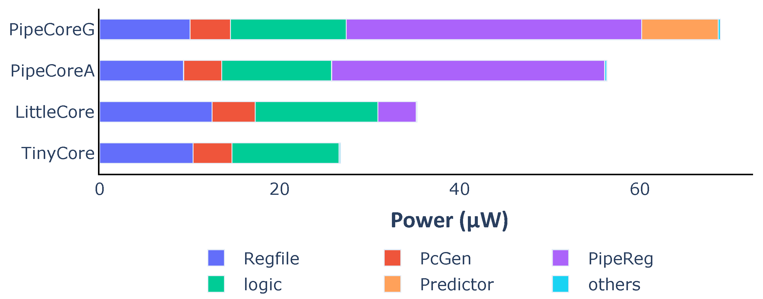
Figure 4 shows the power consumption for each core. Compared to the TinyCore, the other three processors consume 1.32× (LittleCore), 2.11× (PipeCoreA) and 2.58× (PipeCoreG) more power, respectively, on average.
Figure 5 demonstrates the power distribution of all baseline processors. The “logic” part in
Figure 5 represents the power consumption of all necessary combinational circuits, including instruction decoder, execute unit, load data selector, etc. Since the circuits of the “logic” part are essential and their power consumptions are nearly the same in different cores, we will skip that in the following discussion. Note that the RegFile of LittleCore consumes more energy than others, since its better IPC results in more data writing back within the same time frame. Similarly, more power consumption is needed by the RegFile of TinyCore than that of PipeCores.
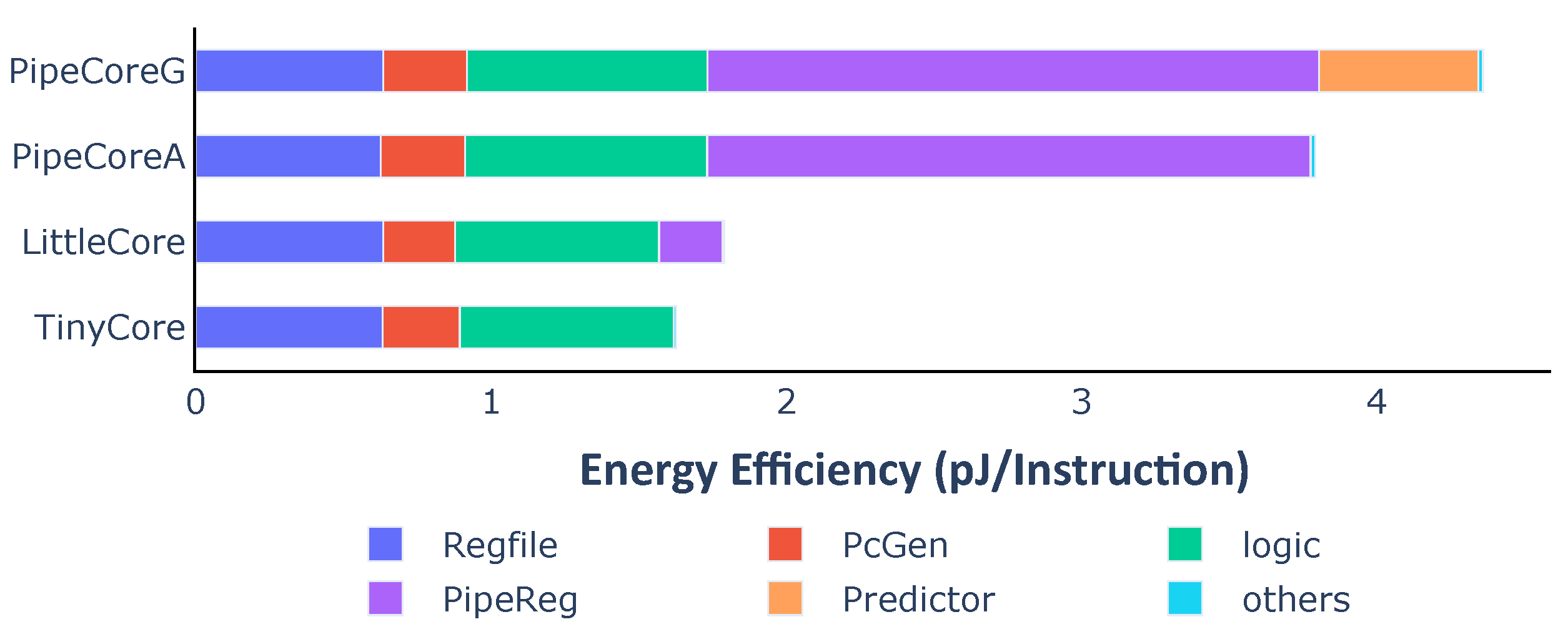
Taking into account the execution efficiency, the distribution of energy efficiency is a bit different from the power consumption.
Figure 6 shows the energy dissipation of each part in a processor for executing one instruction. RegFiles almost consume the same energy in different cores because of the same number of write-backs. PcGenerators and logic circuits in PipeCores consume a little more energy than TinyCore and LittleCore due to the speculative execution. Pipeline registers and the branch predictor have great impacts on energy efficiency. They lead to differences in performance and efficiency among baseline processors.
Pipeline registers. They are not the key contributor to the area, but consume the most energy than other parts in a processor. For example, the area of the pipeline registers is 1.60 KGE that is only 7.54% of the total core in PipeCoreA. However, they need about 1.96 μW/MHz. That is, over 53.9% of total energy (3.63 μW/MHz) is consumed by them. The counterintuitive result is caused by their higher transition frequency.
Branch predictor. The dynamic branch predictor has tremendous impacts on performance, power and energy efficiency. The IPC of PipeCoreG is 0.793 which is 6.34% more than that of PipeCoreA. When running at 20 MHz, the power of PipeCoreG is 68.97 μW. That is 22.38% more than PipeCoreA which consumes 56.36 μW. Thus, the Gshare predictor leads to about 15% more energy dissipation for each instruction.
Considering the performance requirements in embedded systems, a deeper pipeline and dynamic branch predictor are indispensable. However, in low-load scenarios, they become a burden on power. Shutting down these units, when they are not necessary in idle state, will be beneficial for energy efficiency.
4. Architecture and Implementation
4.1. Multiple Operating Modes
Performance and power differ greatly among these baseline processors. An aggressive branch predictor and pipeline structure, which are not essential to complete an instruction, are the main contributors to power increasing. Working without these units will improve energy efficiency. Thus, the ability to run in diverse operating modes is useful for an ultra-low-power processor to balance the performance and energy efficiency.
In the previous section, four baseline cores were discussed. It is not a good idea to support all modes in the design, since more modes may lead to an unnecessary overhead. Among these cores, PipeCoreG has the best performance that is important for many applications. Additionally, the only difference between PipeCoreA and PipeCoreG is the branch predictor. Shutting down the Gshare predictor by inserting several clock gating cells makes the PipeCoreG working like PipeCoreA. Because of the negligible cost, their micro-architectures are both selected as two different modes. The performance of TinyCore is much worse than LittleCore with similar energy efficiency. Therefore, supporting LittleCore only is preferred rather than having two individual modes for them, since additional MUXes are needed for the architecture of TinyCore.
Taking all factors into account, there are three operating modes in the variable architecture processor: (1) High-Performance mode (H-mode). The processor works with a 4-stage pipeline and a Gshare branch predictor. (2) Normal mode (N-mode). The 4-stage pipeline is still employed while shutting down the Gshare predictor. (3) Low-power mode (L-mode). Pipeline registers between Fetch and Execute are all bypassed and no speculative structure is used in this mode. Switching between different modes is controlled by software.
4.2. Variable Branch Predictor
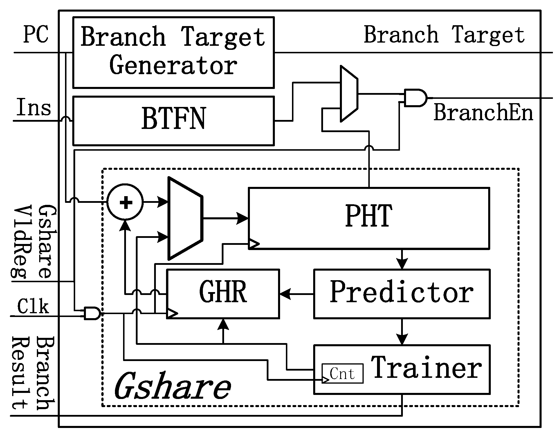
Figure 7 shows the architecture of the variable branch predictor. A memory-mapped register named GshareVldReg is employed in the processor. The branch predictor could work in two different modes indicated by the GshareVldReg.
If GshareVldReg is 1, the prediction result of Gshare is enabled. Prediction is performed in the Decode unit, and the branch target is calculated from the instruction instead of using a branch target buffer (BTB) to avoid additional energy costs. The saturating counter in the Gshare predictor will be out of service when training the pattern history table (PHT), since the PHT SRAM has only one port. Thus, Backward-Taken-Forward-Nottaken(BTFN) prediction is used if a training conflict appears.
When GshareVldReg stays at 0, the Always-Not-Taken algorithm is used. To reduce the energy consumption, the clock to Gshare is gated, and operand isolation is used in the branch target generator. Thus, all the logic circuits, registers and SRAMs keep silent until the operating mode has been changed. In this way, most of the energy could be saved due to the shutting down of Gshare predictor. Only several AND gates are inserted into logic circuits, leading to little costs in terms of area. As these additional gates are not on the critical path, there is no timing overhead for them.
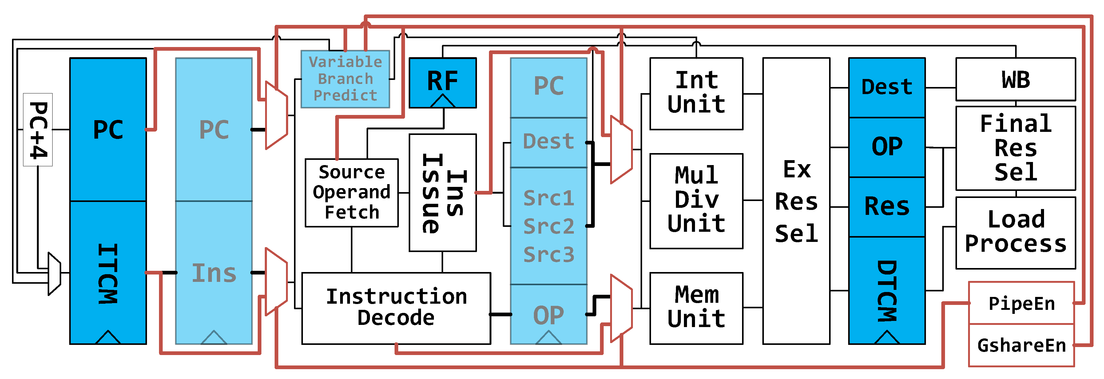
4.3. Variable Pipeline Architecture
Figure 8 demonstrates the variable-architecture processor. It is based on the PipeCore shown in
Figure 2c. To eliminate the wasted energy in pipeline registers, all registers between Fetch and Execute are bypassed, making the core work with a 2-stage pipeline, similarly to the LittleCore mentioned in
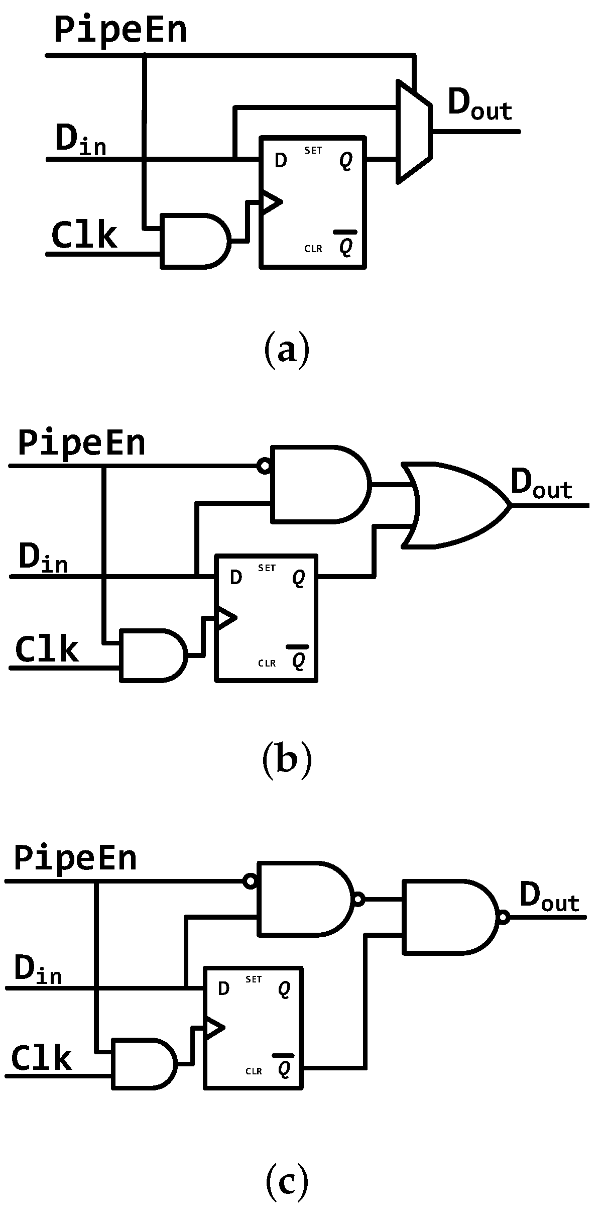
Figure 2b. All bypass transmission is achieved by inserting MUXes after pipeline registers, as shown in
Figure 8 and
Figure 9a. To simplify the MUX circuits, all pipeline registers are flushed to zero before clock gating. Hence, a real multiplexer is not necessary for signal forwarding. We can use an AND-OR gate, as shown in
Figure 9b, instead of a multiplexer. That will reduce the size by one AND gate. Additionally, the AND-OR gate also can be simplified to a NAND-NAND gate by inverting the output of each pipeline register, as shown in
Figure 9c. As a result, only 8 transistors are needed to bypass a signal. That is fewer than a multiplexer (12 transistors) or an AND-OR gate (10 transistors).
A forward bus is used in the 4-stage pipeline architecture to access data before writing them to the register file. In the variable architecture, the destinations of forwarding data come from the pipeline registers directly. In low-power mode, the forwarding data from Execute is invalid, since the pipeline register between Decode and Execute is bypassed, and all bits in the register are flushed to 0. Thus, the destination keeps 5b00000 and the forward bus will be out of service.
In addition to the data path, the execution controlling mechanism in low-power mode is also different. There are no pipeline stalls caused by data hazards in this mode. The controller only stalls the processor when executing multiplication and division, which could take additional cycles. Another memory-mapped register is used to indicate whether the processor is working with or without a complex pipeline structure. The register is named PipeEn, as shown in
Figure 8. When writing 0 to this bit, the processor flushes all pipeline registers between Fetch and Execute, and then blocks the clock to those pipeline registers.
4.4. Software-Based Mode Switching
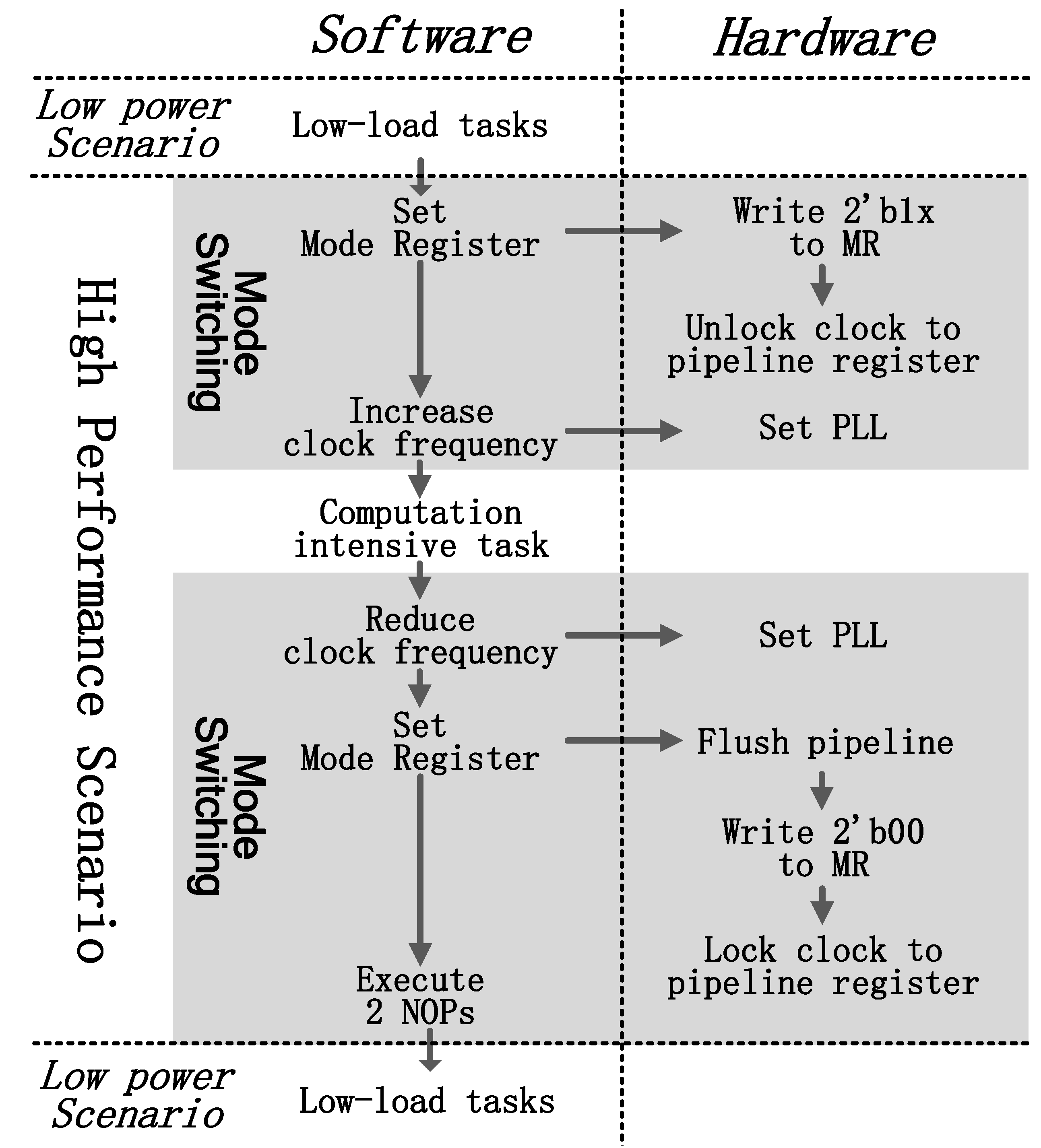
Mode switching is controlled by software. There is a mode register (MR) in the processor indicating current operating mode. PipeEn assigned to bit[1] and GshareEn assigned to bit[0] are used to indicate the pipeline architecture and the type of branch predictor. Note that, there are only three modes in the processor, and therefore writing 2b01 to the mode register is invalid. When the processor switches from L-mode to N-mode or H-mode, the following steps must be done in software:
- 1.
Set mode register to 2b1x (2b10 for N-mode; 2b11 for H-mode).
- 2.
Increase the clock frequency.
- 3.
Jump to compute-intensive tasks.
When switching to L-mode, the following things must be done by software to change the micro-architecture:
- 1.
Reduce the clock frequency.
- 2.
Set MR to 2b00.
- 3.
Execute two NOP instructions.
- 4.
Jump to low-load tasks.
Two extra NOPs are inserted after setting the MR. There are three instructions executing in the pipeline simultaneously besides the MR setting instruction, and the flushing pipeline registers will kill the following two instructions. An example of switching flow is shown in
Figure 10. The processor works in L-mode for low-load tasks at first. When a compute-intensive task is coming, MR is set to 2
b1x in the software. The processor will flush the pipeline registers and unlock their clock. Then it increases the clock frequency and works on the coming tasks. When the tasks are finished, the processor reduces the clock frequency and writes 2
b00 to MR turning to L-mode.
The variable branch predictor could change the prediction algorithm in one cycle and lock or unlock the Gshare predictor next cycle. Switching between H-mode and N-mode only needs two steps in software:
- 1.
Write corresponding data to GshareEn register (bit[0] in MR).
- 2.
Jump to new tasks.
5. Experiment Results and Discussion
We have implemented the variable core in UMC 40LP. It has 26.59 K gates, which is only 7.19% more than PipeCoreG. Additionally, its maximum frequency is 2.3% slower due to the additional NAND cells in the critical path. In low power mode, the maximum frequency is about 260 Mhz. The micro-architectures of the variable core in different operating modes are the same as the corresponding baseline processors. Thus, they have the same execution efficiency evaluated by IPC.
First, we simulated the processor in different modes with a clock frequency of 20 MHz.
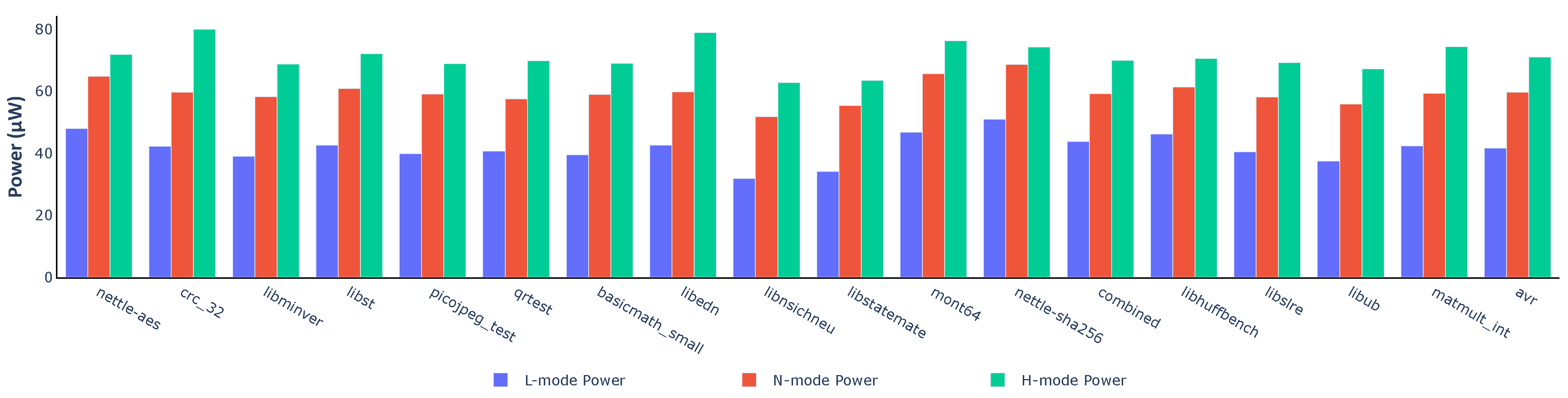
Figure 11 demonstrates the power consumption of each benchmark in Embench. In all cases, working in L-mode reduces power consumption greatly. N-mode also needs less power than H-mode. Compared with H-mode, N-mode and L-mode could save more than 25.36% and 49.30% power in the best cases. Even in the worst cases, about 7.54% and 31.40% power are saved.
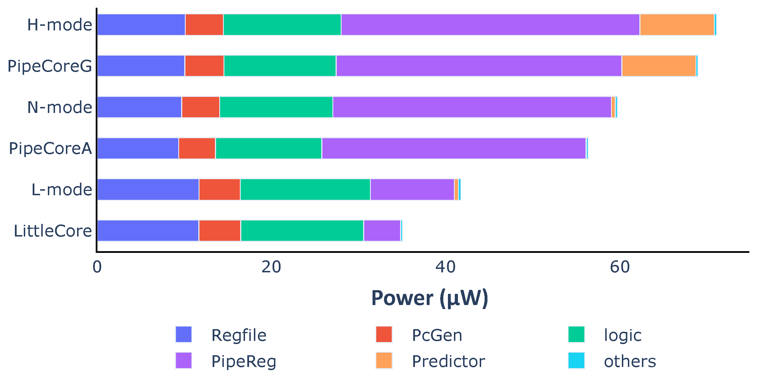
As shown in
Figure 12, the average power of different modes are 41.7 μW, 59.7 μW and 71.1 μW, respectively. Typically, N-mode and L-mode consume 16.08% and 41.37% less power than H-mode within the same clock period. The power consumption of each mode increases a little over the value that is in the corresponding baseline core. This is caused by two reasons: (1) The execution controller in the variable core is a little more complicated than those of TinyCore and LittleCore. Thus, the power of the “logic” part increases a little. (2) Many NAND cells are inserted after some of the pipeline registers, leading to the power increasing in the “PipeReg” part.
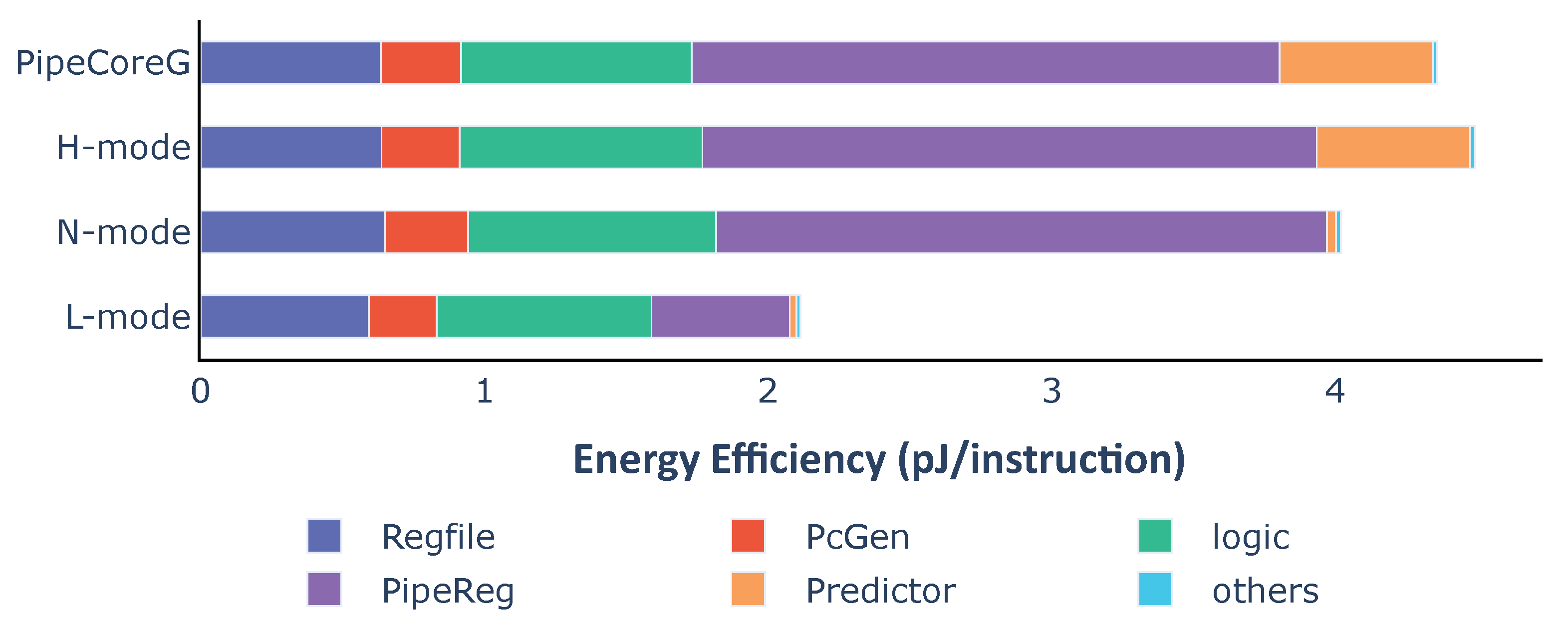
Energy dissipation for each instruction is shown in
Figure 13. To execute one instruction, the variable core in different modes consumes 2.12 pJ (L-mode), 4.02 pJ (N-mode) and 4.50 pJ (H-mode), respectively. For each instruction, the variable core in L-mode needs 52.92% less energy than H-mode. Compared with PipeCoreG consuming 4.36 pJ/instruction, the variable core could save 7.78% and 51.57% more energy in N-mode and L-mode. Only 3.08% more power is consumed in H-mode. According to the power and energy distribution, shutting down the branch predictor saves 0.509 pJ energy which is 92.2% of total energy consumed by the Gshare predictor in PipeCoreG. Bypassing pipeline registers between Fetch and Execute saves 1.585 pJ energy. That is 76.48% of all pipeline registers in PipeCoreG. The energy overhead of H-mode, which is 0.134 pJ, is 3.08% of the total power in PipeCoreG. Most of the additional energy is caused by MUX logics after pipeline registers.
Table 2 shows the peak performance with tight timing constraints and the energy efficiency with relaxed timing constraints for our proposed processor and the state-of-the-art cores. In view of the maximum frequency, the peak performance of the variable core in H-mode and N-mode is better than riscy and Cortex-M4. Additionally, its peak performance in H-mode is a little better than in N-mode due to a better branch predictor. For low-load scenarios, the variable core, working in L-mode, needs less power than zero-riscy and Cortex-M0+. Therefore, the variable core provides a better trade-off between peak performance and energy efficiency, even if the switching circuit involves some power overhead.
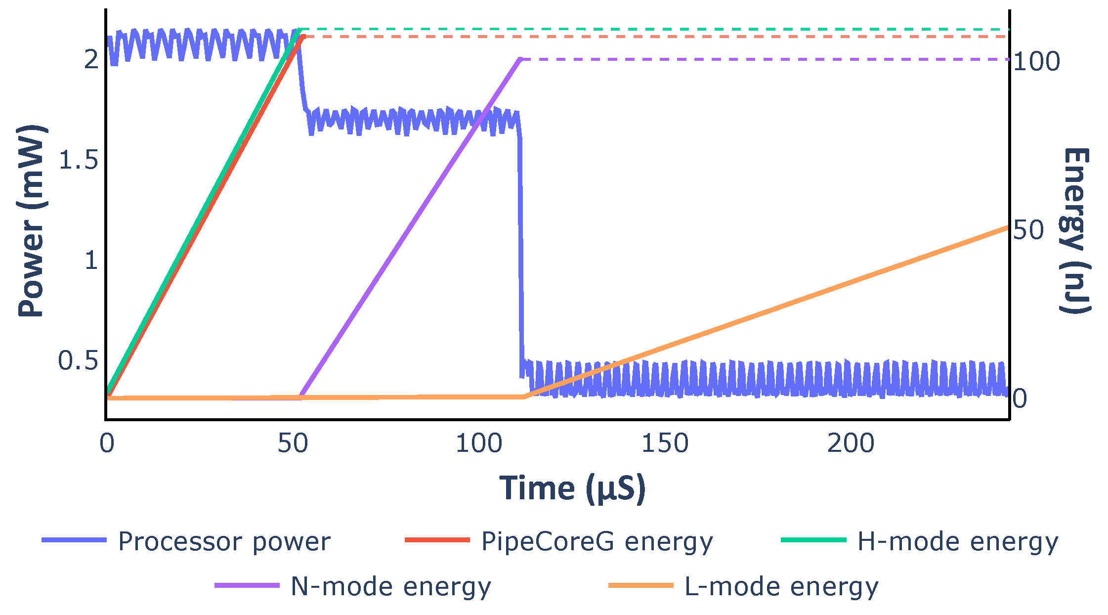
We simulated the variable core with dynamic mode switching. The core executed the Dhrystone benchmark (DMIPS) 50 times in each mode. Energy consumption was calculated by integrating the corresponding power curve. All curves are demonstrated in
Figure 14. The energy curve for PipeCoreG running DMIPS 50 times is also shown in
Figure 14 as a reference. The variable core works at 200 MHz in L-mode, while the other modes and PipeCoreG work at 600 MHz. As the result shows, complicated micro-architectures lead to better peak performance, reducing the execution time for the same task. Simpler micro-architectures improve energy efficiency greatly. Embedded systems could benefit greatly from the variable architecture, if they work on low-load tasks most of the time and handle compute-intensive tasks for only short periods.
6. Conclusions
This paper has analyzed the power distributions of embedded processors with different architectures, and pointed out the key factors reducing energy efficiency. As the results show, the pipeline registers consume 53.9% power with only 7.54% of the total area, and the branch predictor leads to 22.38% more power dissipation with an only 6.34% performance increase. To improve energy efficiency in idle state, a variable processor with three operating modes was proposed in this paper. The core is a 4-stage pipeline processor with a Gshare predictor in high-performance mode. It could shut down unnecessary units in different modes to improve energy efficiency. In normal mode, an Always-Not-Taken predictor is used instead of a Gshare predictor. Additionally, some of the pipeline registers are bypassed in low-power mode.
The variable core, in N-mode and L-mode, consumes 16.08% and 41.37% less power than H-mode on average. Compared with the baseline processor, the proposed processor needs 7.78% and 51.57% less energy to execute one instruction in N-mode and L-mode, respectively. In H-mode, only 3.08% more power is consumed in our design, with 7.19% more gates being involved. The result illustrates that processors with the variable architecture and multiple operating modes will achieve better energy efficiency in various scenarios and meet the demands of peak performance.
For complex tasks in embedded systems, more complicated architectures are employed, such as multi-issue and out-of-order, due to the increase in performance demand. These processors may be simplified by adding new data paths to support architecture switching. For further exploration, our proposed software-controlled variable architecture may also be applied to these complicated processors to balance peak performance and energy efficiency.
Author Contributions
Conceptualization, W.M. and N.Y., Methodology, W.M. and N.Y., Validation, W.M., Q.C., Y.G. and L.X., Formal analysis, Q.C., Investigation, W.M., Writing, W.M., Project administration, N.Y., Funding acquisition, N.Y. All authors have read and agreed to the published version of the manuscript.
Funding
This work was supported in part by the National Natural Science Foundation of China (No. 61771388), and in part by Primary Research& Development Plan of Shaanxi Province, China(2019TSLGY08-03).
Conflicts of Interest
The authors declare no conflict of interest.
References
- Gartner Identifies Top 10 Strategic IoT Technologies and Trends. Available online: https://www.gartner.com/en/newsroom/press-releases/2018-11-07-gartner-identifies-top-10-strategic-iot-technologies-and-trends (accessed on 9 March 2021).
- Shakhsheer, Y.; Zhang, Y.; Otis, B.; Calhoun, B.H. A custom processor for node and power management of a battery-less body sensor node in 130 nm CMOS. In Proceedings of the IEEE 2012 Custom Integrated Circuits Conference, San Jose, CA, USA, 9–12 September 2012; pp. 1–4. [Google Scholar] [CrossRef]
- Su, F.; Chen, W.; Xia, L.; Lo, C.; Tang, T.; Wang, Z.; Hsu, K.; Cheng, M.; Li, J.; Xie, Y.; et al. A 462GOPs/J RRAM-based nonvolatile intelligent processor for energy harvesting IoE system featuring nonvolatile logics and processing-in-memory. In Proceedings of the 2017 Symposium on VLSI Technology, Kyoto, Japan, 5–8 June 2017; pp. T260–T261. [Google Scholar] [CrossRef]
- Beucher, N.; Belanger, N.; Savaria, Y.; Bois, G. A Methodology to Evaluate the Energy Efficiency of Application Specific Processors. In Proceedings of the 2007 14th IEEE International Conference on Electronics, Circuits and Systems, Marrakech, Morocco, 11–14 December 2007; pp. 983–986. [Google Scholar] [CrossRef]
- Rodrigues, R.; Annamalai, A.; Koren, I.; Kundu, S. A Study on the Use of Performance Counters to Estimate Power in Microprocessors. IEEE Trans. Circuits Syst. II Express Briefs 2013, 60, 882–886. [Google Scholar] [CrossRef]
- Fan, Y.; Wu, J.; Wang, S. Efficient energy exploration for embedded systems. In Proceedings of the 18th IEEE International Symposium on Consumer Electronics (ISCE 2014), Jeju, Korea, 22–25 June 2014; pp. 1–2. [Google Scholar] [CrossRef]
- Haque, M.E.; He, Y.; Elnikety, S.; Nguyen, T.D.; Bianchini, R.; McKinley, K.S. Exploiting Heterogeneity for Tail Latency and Energy Efficiency. In Proceedings of the 2017 50th Annual IEEE/ACM International Symposium on Microarchitecture (MICRO), Boston, MA, USA, 14–17 October 2017; pp. 625–638. [Google Scholar]
- ARM Limited. Available online: https://www.arm.com/products/processors/cortex-m (accessed on 9 March 2021).
- Rossi, D.; Conti, F.; Marongiu, A.; Pullini, A.; Loi, I.; Gautschi, M.; Tagliavini, G.; Capotondi, A.; Flatresse, P.; Benini, L. PULP: A parallel ultra low power platform for next generation IoT applications. In Proceedings of the 2015 IEEE Hot Chips 27 Symposium (HCS), Cupertino, CA, USA, 22–25 August 2015; pp. 1–39. [Google Scholar] [CrossRef]
- Gala, N.; Menon, A.; Bodduna, R.; Madhusudan, G.S.; Kamakoti, V. SHAKTI Processors: An Open-Source Hardware Initiative. In Proceedings of the 2016 29th International Conference on VLSI Design and 2016 15th International Conference on Embedded Systems (VLSID), Kolkata, India, 4–8 January 2016; pp. 7–8. [Google Scholar] [CrossRef]
- Zhang, S.; Wright, A.; Bourgeat, T.; Arvind, A. Composable Building Blocks to Open up Processor Design. In Proceedings of the 2018 51st Annual IEEE/ACM International Symposium on Microarchitecture (MICRO), Fukuoka, Japan, 20–24 October 2018; pp. 68–81. [Google Scholar] [CrossRef]
- Hoang, T.T.; Duran, C.; Nguyen, K.D.; Dang, T.K.; Nhu, Q.N.Q.; Than, P.H.; Tran, X.T.; Le, D.H.; Tsukamoto, A.; Suzaki, K.; et al. Low-power high-performance 32-bit RISC-V microcontroller on 65-nm silicon-on-thin-BOX (SOTB). IEICE Electron. Express 2020, 17, 20200282. [Google Scholar] [CrossRef]
- Rovinski, A.; Zhao, C.; Al-Hawaj, K.; Gao, P.; Xie, S.; Torng, C.; Davidson, S.; Amarnath, A.; Vega, L.; Veluri, B.; et al. A 1.4 GHz 695 Giga Risc-V Inst/s 496-Core Manycore Processor With Mesh On-Chip Network and an All-Digital Synthesized PLL in 16nm CMOS. In Proceedings of the 2019 Symposium on VLSI Circuits, Kyoto, Japan, 9–14 June 2019; pp. C30–C31. [Google Scholar] [CrossRef]
- Matthews, E.; Shannon, L. TAIGA: A new RISC-V soft-processor framework enabling high performance CPU architectural features. In Proceedings of the 2017 27th International Conference on Field Programmable Logic and Applications (FPL), Ghent, Belgium, 4–8 September 2017; pp. 1–4. [Google Scholar] [CrossRef]
- Gautschi, M.; Schiavone, P.D.; Traber, A.; Loi, I.; Pullini, A.; Rossi, D.; Flamand, E.; Gürkaynak, F.K.; Benini, L. Near-Threshold RISC-V Core With DSP Extensions for Scalable IoT Endpoint Devices. IEEE Trans. Very Large Scale Integr. (VLSI) Syst. 2017, 25, 2700–2713. [Google Scholar] [CrossRef]
- Flamand, E.; Rossi, D.; Conti, F.; Loi, I.; Pullini, A.; Rotenberg, F.; Benini, L. GAP-8: A RISC-V SoC for AI at the Edge of the IoT. In Proceedings of the 2018 IEEE 29th International Conference on Application-specific Systems, Architectures and Processors (ASAP), Milan, Italy, 10–12 July 2018; pp. 1–4. [Google Scholar] [CrossRef]
- Eggimann, M.; Mach, S.; Magno, M.; Benini, L. A RISC-V Based Open Hardware Platform for Always-On Wearable Smart Sensing. In Proceedings of the 2019 IEEE 8th International Workshop on Advances in Sensors and Interfaces (IWASI), Otranto, Italy, 13–14 June 2019; pp. 169–174. [Google Scholar] [CrossRef]
- Mach, S.; Schuiki, F.; Zaruba, F.; Benini, L. A 0.80pJ/flop, 1.24Tflop/sW 8-to-64 bit Transprecision Floating-Point Unit for a 64 bit RISC-V Processor in 22nm FD-SOI. In Proceedings of the 2019 IFIP/IEEE 27th International Conference on Very Large Scale Integration (VLSI-SoC), Cusco, Peru, 6–9 October 2019; pp. 95–98. [Google Scholar] [CrossRef]
- Zaruba, F.; Benini, L. The Cost of Application-Class Processing: Energy and Performance Analysis of a Linux-Ready 1.7-GHz 64-Bit RISC-V Core in 22-nm FDSOI Technology. IEEE Trans. Very Large Scale Integr. (VLSI) Syst. 2019, 27, 2629–2640. [Google Scholar] [CrossRef]
- ARM Cortex-M0+. Available online: https://developer.arm.com/ip-products/processors/cortex-m/cortex-m0-plus (accessed on 9 March 2021).
- ARM Cortex-M3. Available online: https://developer.arm.com/ip-products/processors/cortex-m/cortex-m3 (accessed on 9 March 2021).
- ARM Cortex-M4. Available online: https://developer.arm.com/ip-products/processors/cortex-m/cortex-m4 (accessed on 9 March 2021).
- ARM Cortex-M7. Available online: https://developer.arm.com/ip-products/processors/cortex-m/cortex-m7 (accessed on 9 March 2021).
- Chang, J.; Pedram, M. Energy minimization using multiple supply voltages. IEEE Trans. Very Large Scale Integr. (VLSI) Syst. 1997, 5, 436–443. [Google Scholar] [CrossRef]
- Usami, K.; Igarashi, M.; Minami, F.; Ishikawa, T.; Kanzawa, M.; Ichida, M.; Nogami, K. Automated low-power technique exploiting multiple supply voltages applied to a media processor. IEEE J. Solid-State Circuits 1998, 33, 463–472. [Google Scholar] [CrossRef]
- Horowitz, M. 1.1 Computing’s energy problem (and what we can do about it). In Proceedings of the 2014 IEEE International Solid-State Circuits Conference Digest of Technical Papers (ISSCC), San Francisco, CA, USA, 9–13 February 2014; pp. 10–14. [Google Scholar]
- Balakrishnan, S.; Rajwar, R.; Upton, M.; Lai, K. The impact of performance asymmetry in emerging multicore architectures. In Proceedings of the 32nd International Symposium on Computer Architecture (ISCA’05), Madison, WI, USA, 4–8 June 2005; pp. 506–517. [Google Scholar] [CrossRef]
- Kumar, R.; Farkas, K.I.; Jouppi, N.P.; Ranganathan, P.; Tullsen, D.M. Single-ISA heterogeneous multi-core architectures: The potential for processor power reduction. In Proceedings of the 36th Annual IEEE/ACM International Symposium on Microarchitecture, 2003, MICRO-36, San Diego, CA, USA, 3–5 December 2003; pp. 81–92. [Google Scholar] [CrossRef]
- Kumar, R.; Tullsen, D.M.; Ranganathan, P.; Jouppi, N.P.; Farkas, K.I. Single-ISA heterogeneous multi-core architectures for multithreaded workload performance. In Proceedings of the 31st Annual International Symposium on Computer Architecture, Munich, Germany, 23 June 2004; pp. 64–75. [Google Scholar] [CrossRef]
- Kumar, R.; Tullsen, D.M.; Jouppi, N.P. Core architecture optimization for heterogeneous chip multiprocessors. In Proceedings of the 2006 International Conference on Parallel Architectures and Compilation Techniques (PACT), Seattle, WA, USA, 16–20 September 2006; pp. 23–32. [Google Scholar]
- Kuroda, T.; Suzuki, K.; Mita, S.; Fujita, T.; Yamane, F.; Sano, F.; Chiba, A.; Watanabe, Y.; Matsuda, K.; Maeda, T.; et al. Variable supply-voltage scheme for low-power high-speed CMOS digital design. IEEE J. Solid-State Circuits 1998, 33, 454–462. [Google Scholar] [CrossRef]
- Agwa, S.; Yahya, E.; Ismail, Y. Power efficient AES core for IoT constrained devices implemented in 130 nm CMOS. In Proceedings of the 2017 IEEE International Symposium on Circuits and Systems (ISCAS), Baltimore, MD, USA, 28–31 May 2017; pp. 1–4. [Google Scholar] [CrossRef]
- Kim, W.; Gupta, M.S.; Wei, G.; Brooks, D. System level analysis of fast, per-core DVFS using on-chip switching regulators. In Proceedings of the 2008 IEEE 14th International Symposium on High Performance Computer Architecture, Salt Lake City, UT, USA, 16–20 February 2008; pp. 123–134. [Google Scholar]
- Burd, T.D.; Pering, T.A.; Stratakos, A.J.; Brodersen, R.W. A dynamic voltage scaled microprocessor system. IEEE J. Solid-State Circuits 2000, 35, 1571–1580. [Google Scholar] [CrossRef]
- Annavaram, M.; Grochowski, E.; Shen, J. Mitigating Amdahl’s law through EPI throttling. In Proceedings of the 32nd International Symposium on Computer Architecture (ISCA’05), Madison, WI, USA, 4–8 June 2005; pp. 298–309. [Google Scholar] [CrossRef]
- Vasilakis, E.; Sourdis, I.; Papaefstathiou, V.; Psathakis, A.; Katevenis, M.G.H. Modeling energy-performance tradeoffs in ARM big.LITTLE architectures. In Proceedings of the 2017 27th International Symposium on Power and Timing Modeling, Optimization and Simulation (PATMOS), Thessaloniki, Greece, 25–27 September 2017; pp. 1–8. [Google Scholar] [CrossRef]
- Sayadi, H.; Pathak, D.; Savidis, I.; Homayoun, H. Power conversion efficiency-aware mapping of multithreaded applications on heterogeneous architectures: A comprehensive parameter tuning. In Proceedings of the 2018 23rd Asia and South Pacific Design Automation Conference (ASP-DAC), Jeju, Korea, 22–25 January 2018; pp. 70–75. [Google Scholar] [CrossRef]
- Chronaki, K.; Moretó, M.; Casas, M.; Rico, A.; Badia, R.M.; Ayguadé, E.; Valero, M. On the maturity of parallel applications for asymmetric multi-core processors. J. Parallel Distrib. Comput. 2019, 127, 105–115. [Google Scholar] [CrossRef]
- Edun, A.; Vazquez, R.; Gordon-Ross, A.; Stitt, G. Dynamic Scheduling on Heterogeneous Multicores. In Proceedings of the 2019 Design, Automation Test in Europe Conference Exhibition (DATE), Florence, Italy, 25–29 March 2019; pp. 1685–1690. [Google Scholar] [CrossRef]
- Lukefahr, A.; Padmanabha, S.; Das, R.; Sleiman, F.M.; Dreslinski, R.G.; Wenisch, T.F.; Mahlke, S. Composite Cores: Pushing Heterogeneity Into a Core. In Proceedings of the 2012 45th Annual IEEE/ACM International Symposium on Microarchitecture, Vancouver, BC, Canada, 1–5 December 2012; pp. 317–328. [Google Scholar]
- Srinivasan, S.; Kurella, N.; Koren, I.; Kundu, S. Exploring Heterogeneity within a Core for Improved Power Efficiency. IEEE Trans. Parallel Distrib. Syst. 2016, 27, 1057–1069. [Google Scholar] [CrossRef]
- Davide Schiavone, P.; Conti, F.; Rossi, D.; Gautschi, M.; Pullini, A.; Flamand, E.; Benini, L. Slow and steady wins the race? A comparison of ultra-low-power RISC-V cores for Internet-of-Things applications. In Proceedings of the 2017 27th International Symposium on Power and Timing Modeling, Optimization and Simulation (PATMOS), Thessaloniki, Greece, 25–27 September 2017; pp. 1–8. [Google Scholar]
- Embench: A Modern Embedded Benchmark Suite. Available online: https://www.embench.org/ (accessed on 9 March 2021).
- Arm Ltd. Arm Cortex-M0+ Processor Datasheet; Arm Ltd.: San Jose, CA, USA, 2020. [Google Scholar]
- Arm Ltd. Arm Cortex-M4 Processor Datasheet; Arm Ltd.: San Jose, CA, USA, 2020. [Google Scholar]
Figure 1.
Performance, power and energy efficiency of Cortex-M cores and Pulp cores. (a) Performance of Cortex-M Cores and Pulp Cores, (b) Power of Cortex-M Cores and Pulp Cores, (c) Energy Efficiency of Cortex-M Cores and Pulp Cores.
Figure 1.
Performance, power and energy efficiency of Cortex-M cores and Pulp cores. (a) Performance of Cortex-M Cores and Pulp Cores, (b) Power of Cortex-M Cores and Pulp Cores, (c) Energy Efficiency of Cortex-M Cores and Pulp Cores.
Figure 2.
Architecture of baseline processors. (a) Architecture of TinyCore, (b) Architecture of LittleCore, (c) Architecture of PipeCore.
Figure 2.
Architecture of baseline processors. (a) Architecture of TinyCore, (b) Architecture of LittleCore, (c) Architecture of PipeCore.
Figure 3.
Instructions per cycle (IPC) of baseline Processors.
Figure 3.
Instructions per cycle (IPC) of baseline Processors.
Figure 4.
Power consumption of baseline processors.
Figure 4.
Power consumption of baseline processors.
Figure 5.
Average power consumption and distribution of baseline processors.
Figure 5.
Average power consumption and distribution of baseline processors.
Figure 6.
Average energy consumption and distribution of baseline processors.
Figure 6.
Average energy consumption and distribution of baseline processors.
Figure 7.
Variable branch predictor.
Figure 7.
Variable branch predictor.
Figure 8.
Variable architecture. Pipeline registers and branch predictor can be disabled in normal mode (N-mode) and low-power mode (L-mode). They are translucent in the figure.
Figure 8.
Variable architecture. Pipeline registers and branch predictor can be disabled in normal mode (N-mode) and low-power mode (L-mode). They are translucent in the figure.
Figure 9.
Bypass circuits for each pipeline register. (a) MUX Bypass, (b) AND-OR Bypass, (c) NAND-NAND Bypass.
Figure 9.
Bypass circuits for each pipeline register. (a) MUX Bypass, (b) AND-OR Bypass, (c) NAND-NAND Bypass.
Figure 10.
Software-based mode switching flow.
Figure 10.
Software-based mode switching flow.
Figure 11.
Power consumption of the variable processor in different modes.
Figure 11.
Power consumption of the variable processor in different modes.
Figure 12.
Average power consumption and distribution of the variable processor in different modes.
Figure 12.
Average power consumption and distribution of the variable processor in different modes.
Figure 13.
Average energy consumption and distribution of the variable processor in different modes.
Figure 13.
Average energy consumption and distribution of the variable processor in different modes.
Figure 14.
Dynamic power and energy for DMIPS.
Figure 14.
Dynamic power and energy for DMIPS.
Table 1.
Comparison of baseline processors and the state-of-the-art cores.
Table 1.
Comparison of baseline processors and the state-of-the-art cores.
| Core Name | Pipe No. | Hard Mul Div | Technology | Power Supply | Area (KGE) | Perf (CoreMark/MHz) | Power (W/MHz) |
|---|
| TinyCore | / | Y | 40 nm | 1.1 V | 19.3 | 2.88 | 2.12 |
| LittleCore | 2 | Y | 40 nm | 1.1 V | 19.8 | 3.44 | 2.29 |
| PipeCoreA | 4 | Y | 40 nm | 1.1 V | 21.2 | 2.75 | 3.63 |
| PipeCoreG | 4 | Y | 40 nm | 1.1 V | 24.8 | 2.91 | 5.32 |
| micro-riscy | 2 | N | 65 nm | 1.2 V | 11.6 | 0.91 | 2.33 |
| zero-riscy | 2 | Y | 65 nm | 1.2 V | 18.9 | 2.44 | 2.81 |
| riscy | 4 | Y | 65 nm | 1.2 V | 40.7 | 3.19 | 6.98 |
| Cortex-M0+ | 2 | Y | 40 nm | 1.1 V | 12.5 | 2.46 | 3.8 |
| Cortex-M3 | 3 | Y | 40 nm | 1.1 V | 37.9 | 3.34 | 11 |
| Cortex-M4 | 3 | Y | 40 nm | 1.1 V | 53 | 3.42 | 12.26 |
Table 2.
Comparison with the state-of-the-art processors.
Table 2.
Comparison with the state-of-the-art processors.
| Core Name | Technology | Power
Supply | Area
(KGE) | Performance
(CoreMark/MHz) | Max Frequency
(MHz) | Power
(μW/MHz) | Peak Performance
(CoreMark/s) | Efficiency
(μW/CoreMark) |
|---|
| Variable Core(L-mode) | 40 nm | 1.1 V | 25.9 | 3.44 | 260 | 3.12 | 894 | 0.91 |
| Variable Core(N-mode) | 40 nm | 1.1 V | 25.9 | 2.75 | 700 | 4.50 | 1925 | 1.64 |
| Variable Core(H-mode) | 40 nm | 1.1 V | 25.9 | 2.91 | 700 | 5.49 | 2037 | 1.89 |
| PipeCoreG | 40 nm | 1.1 V | 24.8 | 2.91 | 720 | 5.32 | 2095 | 1.83 |
| zero-riscy [42] | 65 nm | 1.2 V | 18.9 | 2.44 | 560 | 2.81 | 1366 | 1.15 |
| riscy [42] | 65 nm | 1.1 V | 40.7 | 3.19 | 560 | 6.98 | 1786 | 2.19 |
| Cortex-M0+ [44] | 40 nm | 1.1 V | 12.5 | 2.46 | 297 | 3.8 | 730 | 1.54 |
| Cortex-M4 [45] | 40 nm | 1.1 V | 53 | 3.42 | 223 | 12.26 | 762 | 3.58 |
| Publisher’s Note: MDPI stays neutral with regard to jurisdictional claims in published maps and institutional affiliations. |
© 2021 by the authors. Licensee MDPI, Basel, Switzerland. This article is an open access article distributed under the terms and conditions of the Creative Commons Attribution (CC BY) license (http://creativecommons.org/licenses/by/4.0/).


