Investigation of Shear-Driven and Pressure-Driven Liquid Crystal Flow at Microscale: A Quantitative Approach for the Flow Measurement

Abstract

The liquid crystal-based method is a new technology developed for flow visualizations and measurements at microscale with great potentials. It is the priority to study the flow characteristics before implementation of such a technology. A numerical analysis has been applied to solve the simplified dimensionless two-dimensional Leslie–Ericksen liquid crystal dynamic equation. This allows us to analyze the coupling effect of the LC’s director orientation and flow field. We will be discussing two classic shear flow cases at microscale, namely Couette and Poiseuille flow. In both cases, the plate drag speed in the state of Couette flow are varied as well as the pressure gradients in Poiseuille flow state are changed to study their effects on the flow field distributions. In Poiseuille flow, with the increase of applied pressure gradient, the influence of backflow significantly affects the flow field. Results show that the proposed method has great advantages on measurement near the wall boundaries which could complement to the current adopted flow measurement technique. The mathematical model proposed in this article could be of great potentials in the development of the quantitatively flow measurement technology.

1. Introduction

Thermotropic liquid crystals (LCs) are a mesophase exhibiting the appearance of an anisotropic liquid whose molecules represent in rodlike or discotic shape [1]. Its unique features are the temperature dependent nature, whose phase transitions are controlled by the temperature. For thermotropic LCs, the liquid crystals in nematic phase attracts tremendous attention [2]. Among them, the rod like molecules with large length-to-diameter ratio, and no long range order in the molecular centroid are the most common ones. Due to the presence of the rod-shaped molecules, the fluid translational motion is coupled with the internal orientational motion of molecules. Hence, their flow properties can be much richer than simple Newtonian fluids. Conversely, the change of molecular orientation order affects the flow in return. This coupling has important practical consequences upon the application of LCs [3]. Therefore, investigations on mechanism of hydrodynamic shear induced reorientation of the liquid crystal molecules are necessary. The research of the T.G. Anderson team focuses on the physical change of liquid crystal fluid under microfluid channel with pressure gradient [4]. The team studies the transformation process of the two states of liquid crystal fluid by numerical calculation and compares the results of the transition of the flow state with the experiment of the Sengupta team [5]. The dimensionless equation is obtained through normalization, which makes the results more intuitive and more universal. In addition, the elastic free energy of liquid crystals in different states is presented. The reasons for the change of liquid crystal flow state are well explained by the comparison of the elastic free energy [5]. Compared to the fluid flow at marcoscale, flow at microscale (mostly in microchannels here) is fundamentally different due to the limited inertial effects and dominating viscous stress and interfacial tension.

In this paper, we choose 4-Cyano-4′-pentylbiphenyl (5CB) as which stays in nematic phase under room temperature. 5CB is a type of nematic liquid crystal (NLC) called “calamitics” [6] which represents the rod-like molecular structure. The structure can be observed experimentally using the polarized microscopy configuration. Recent literatures have been focusing more on the characteristic response to the electric field [7,8,9,10]. The well-known orientation Fredericks transition has been extensively studied and applied in practical applications [11]. Furthermore, the combination of the delicate microscale fluidic control with LCs, especially the nematic LCs has allowed the possibility of topological studies [12], phase transitions [13,14,15,16]and the unique stripe structure [17,18]. More importantly, it also leads to the diverse application in fields of microfabrications, 3D printing and bioengineering [12,13,19,20]. Nonetheless, very few works have been reported on the reorientation influenced by the hydrodynamic pressure at microscale [21,22,23]. Currently, the most commonly used model to study directional vector deflection and flow of nematic liquid crystals is the Leslie–Ericksen equations (L-E equation). We apply the Leslie–Ericksen formalism for nematodynamics to investigate the shear flow model. First, we describe the model of the liquid crystal by means of L-E equations [24]. The analysis is restricted to the steady state deformations of the nematic phase where α₃/α₂ > 0. The flow behavior of nematic liquid crystals can be generally categorized into two major types through the signs of the two Leslie viscosities α₂ and α₃. If α₃/α₂ > 0, then the liquid crystal is flow aligning, otherwise it is flow tumbling [25]. Next, we addressed two typical steady 2D cases: the shear-driven (Couette) and the pressure-driven (Poiseuille) flow of nematic liquid crystal in a parallel microchannel respectively. Then we applied justified assumptions for simplification purpose before solving them numerically. The director profile is calculated for various pressure gradients and shear stresses. For pressure-driven flow cases, we find that under the limitation of strong anchoring and weak flow effects, flow alignment is not presented. In fact, the director field is majorly determined by the boundary conditions. For other cases, the results clearly show the influence of flow condition on reorientation of director field, which provide guideline for flow measurements at microscale [26,27,28].

2. Mathematical Models

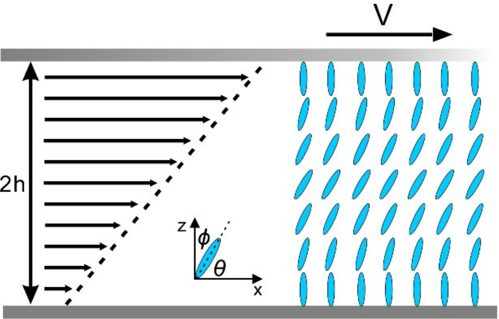
There are two major differences considering the hydrodynamics of simple Newtonian fluids and that of the LCs. First, LCs’ molecules can be rotated by the pressure gradient due to its unique geometries. Second, the equilibrium free energy of LCs is more complex. This coupling between the elastic energy and the flow, which is called backflow, leads to rich hydrodynamic behaviors. In order to seize the main physical properties of LCs, the details of the molecules are neglected and the ideal approximation is processed. For example, for nematic LCs, LC molecules are often idealized as a long rod with a symmetric head and tail, and hence uniaxial symmetry. As mentioned earlier, LCs molecules are anisotropic, therefore we need to introduce variables called order parameter to describe the alignment and orientation of LCs. We adopt the well accepted Leslie–Ericksen model to describe the director orientation and LC flow. In the continuum theory, we define the orientation of the LCs at a point by a unit vector n called the director.

The full equation of nematodynamics consists of

$$V_{i,i}=0$$

(1)

$$\rho {\overrightarrow{v}}_i=\rho F_i-{(p+W_F)}_{,i}+{\tilde{g}}_j{n}_{j,i}+G_j{n}_{j,i}+{\tilde{t}}_{ij,j}$$

(2)

$${\left(\frac{\partial W_F}{\partial n_{i,j}}\right)}_j-\frac{\partial W_F}{\partial n_i}+{\tilde{g}}_i+G_i=\lambda n_i$$

(3)

Representing mass, energy, and momentum conservations respectively. We consider a steady 2D plane Poiseuille–Couette flow of nematic liquid crystal in a microfluidic channel with two parallel boundaries and a thin film geometry. The upper plate travels along the x direction at a constant speed V (shear-driven flow) or a constant pressure gradient is applied within the LCs (pressure-driven flow) as shown in Figure 1 and Figure 2 respectively.

2.1. Couette Flow

It will be assumed that the director and the velocity take the forms

$$\overrightarrow{n}=[\cos \theta (z),0,\sin \theta (z)]$$

(4)

$$\overrightarrow{v}=[v(z),0,0]$$

(5)

We now investigate the coquette flow at a fixed distance, d = 2h where the lower plate is at rest and the upper plate is moving at a constant velocity V as shown in Figure 1. Three assumptions are listed as follows (Macsithigh, G. P, and P. K. Currie, 1977):

The one-constant approximation applied to the Oseen–Zocher–Frank elastic free energy equation. In details K₁₁ = K₂₂ = K₃₃ ≡ K, where K₁₁ is the splay coefficient, K₂₂ is the twist coefficient, and K₃₃ is the bend coefficient. (Currie, P. K., and G. P. Macsithigh, 1979).

Parodi’s relation [29]

$${\alpha }_6={\alpha }_5+{\alpha }_3+{\alpha }_2$$

(6)

The zero viscosity coefficient${\mathsf{\alpha }}_1=0$.

From the (2), (3) and the assumptions, it follows that

$$\frac{dv}{dz}=\frac{c}{g(\theta )}$$

(7)

$$2K\frac{d^2\theta }{d{z}^2}-c\frac{[{\gamma }_1+{\gamma }_2\cos (2\theta )]}{g(\theta )}=0$$

(8)

$$g(\theta )=\frac{1}{2}[{\alpha }_5-{\alpha }_2+{\alpha }_4+2({\alpha }_3+{\alpha }_2){\cos }^2\theta ]$$

(9)

For simplicity we nondimensionalize the equations by using the scaling lengths with half-width of the channel h, the velocity $\overline{v}$ with $\overline{v}=V/2$, and all viscosities ${\gamma }_i {\alpha }_i$ with${\alpha }_4$. The dimensionless governing equations become:

$$\frac{d^2\theta }{d{z}^2}=\frac{Vh{\alpha }_4}{4K}\frac{({\alpha }_5+1+{\alpha }_2+2{\alpha }_3)({\gamma }_1+{\gamma }_2\cos 2\theta )}{{\alpha }_5+1-{\alpha }_2+2({\alpha }_2+{\alpha }_3){\cos }^2\theta }$$

(10)

$$\frac{d^2\mathrm{v}}{d{z}^2}=\frac{({\alpha }_5+1+{\alpha }_2+2{\alpha }_3)\sin 2\theta }{{[{\alpha }_5+1-{\alpha }_2+2({\alpha }_2+{\alpha }_3){\cos }^2\theta ]}^2}{\theta }^{\prime }$$

(11)

where ${\gamma }_1={\alpha }_3-{\alpha }_{2 , }{\gamma }_2={\alpha }_6-{\alpha }_5$, the ${\alpha }_i$ are constant viscosities for the NLC. The director is strongly anchored parallel to the plates at the boundaries (Leslie, F.M. 1979), and that the solution for Φ is symmetric in z. A more detailed derivation process can be refereed to Appendix A and Appendix B for Couette flow.

We applied the boundary conditions as: $v\left(-1\right)=0$, $v\left(1\right)=2$,$\theta \left(-1\right)=\theta \left(1\right)=П$/2.

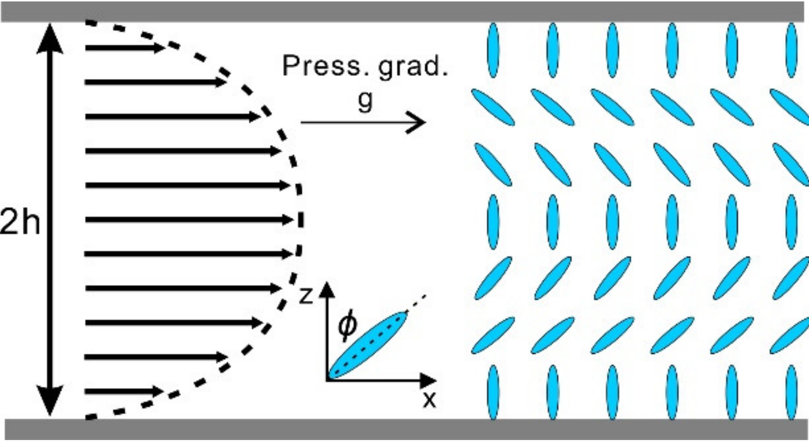
2.2. Poiseuille Flow

Here we consider the steady 2D Poiseuille flow in a microfluidic channel $-h\le z\le h$ as schemed in Figure 2. To investigate a typical, two-dimensional shear flow behavior, the director and the velocity take the forms

$$\overrightarrow{n}=[\sin \varphi (z),0,\cos \varphi (z)]$$

(12)

$$\overrightarrow{v}=[v(z),0,0]$$

(13)

In order to simplify the boundary conditions, it is assumed that Φ is the angle between z axis and the molecule axis (Figure 2). We use the first two assumption ${\alpha }_6={\alpha }_5+{\alpha }_3+{\alpha }_2$ and $K1=K3=K$. Therefore, the following formulas can be obtained

$$\frac{dv}{dz}=\frac{c}{g(\varphi )}$$

(14)

$$2K\frac{d^2\varphi }{d{z}^2}+c\frac{[{\gamma }_1-{\gamma }_2\cos (2\varphi )]}{g(\varphi )}=0$$

(15)

$$g(\varphi )=\frac{1}{2}[2{\alpha }_1{\sin }^2\varphi {\cos }^2\varphi +({\alpha }_5-{\alpha }_2){\cos }^2\varphi +({\alpha }_3+{\alpha }_6){\sin }^2\varphi +{\alpha }_4]$$

(16)

where ${\gamma }_1={\alpha }_3-{\alpha }_{2 , }{\gamma }_2={\alpha }_6-{\alpha }_5$, the ${\alpha }_i$ are constant viscosities for the NLC.

To nondimensionalize the equations, we adopted the following strategies: scale the physical length with the half width of the channel h, the velocity v with $\overline{v}=2G{h}^2/3{\alpha }_4$(Anderson, T. G. et al., 2015), and all viscosities ${\gamma }_i, {\alpha }_i$ with${\alpha }_4$. The dimensionless form of the governing equations become,

$$\frac{\mathrm{dv}}{dz}=-\frac{3z}{\left[2{\alpha }_1{\sin }^2\varphi {\cos }^2\varphi +\left({\alpha }_5-{\alpha }_2\right){\cos }^2\varphi +\left({\alpha }_3+{\alpha }_6\right){\sin }^2\varphi +1\right]}$$

(17)

$$\frac{\varphi ’’\left(z\right)}{{\gamma }_1-{\gamma }_2\cos 2\varphi }\left[2{\alpha }_1{\sin }^2\varphi {\cos }^2\varphi +\left({\alpha }_5-{\alpha }_2\right){\cos }^2\varphi +\left({\alpha }_3+{\alpha }_6\right){\sin }^2\varphi +1\right]=gz$$

(18)

where g = Gh³/K is a dimensionless pressure gradient.

It is assumed that the director is strongly anchored vertically and uniform to the plates at the boundaries before the flow turned on and the solution for Φ is symmetric in z.

The director profile across the dimensionless channel width −1≤ z ≤ 1 under strong anchoring and g = 25 is calculated in Figure 3a to compare with the results obtained by Anderson team (Anderson, T. G. et al., 2015) in Figure 3b. The calculated deflection angle of liquid crystal is in good agreement with the results in the research content of Anderson team.

3. Results

We compute solutions of the system by choosing parameters for the liquid crystal 5CB (Sengupta, A, et al., 2013) in the nematic phase. The dimensionless viscosities chosen are ${\alpha }_1=-0.1594$, ${\alpha }_2=-0.9859$, ${\alpha }_3=-0.0535$, ${\alpha }_5=0.7324$, ${\alpha }_6=-0.3944$, $\mathrm{K}=4\times {10}^{-12} N$; and ${\gamma }_1={\alpha }_3-{\alpha }_2$, ${\gamma }_2={\alpha }_6-{\alpha }_5$. Equation is solved using fourth-order Runge–Kutta integration and the shooting method.

3.1. Couette Flow

In this section, we conducted a systematic parametric investigation on velocity and director fields of a nematic liquid crystal under the shear controlled by the velocity V of the upper plate. The height of the channel was setup as 10 µm. The computations were carried out for different velocities of the upper plane.

Figure 4a shows director profiles when the velocity of the upper plate is 10 µm/s, 100 µm/s, 250 µm/s, and 350 µm/s respectively. It can be seen in Figure 4a that the director profile is almost an axisymmetric parabola at the center. With increasing of the velocity, the angle of the director becomes smaller which is more flow orientated. In Figure 4b, the mid-plane angles ${\varnothing }_m$are plotted as functions of velocity V. We found that the mid-plane angles ${\varnothing }_m$ tend to ${\varnothing }_c$=arctan[(α₃/α₂)^0.5] (${\varnothing }_c$= 0.22, in this article) with the increasing velocity, which agrees with the continuum theory proposed by Leslie and Ericksen [30]. Leslie defined the Leslie angle as: “for which there is no hydrodynamic torque on the director in simple shear flow of an infinitely thick sample”. It is found in this article that the Leslie angle still exists in microchannel.

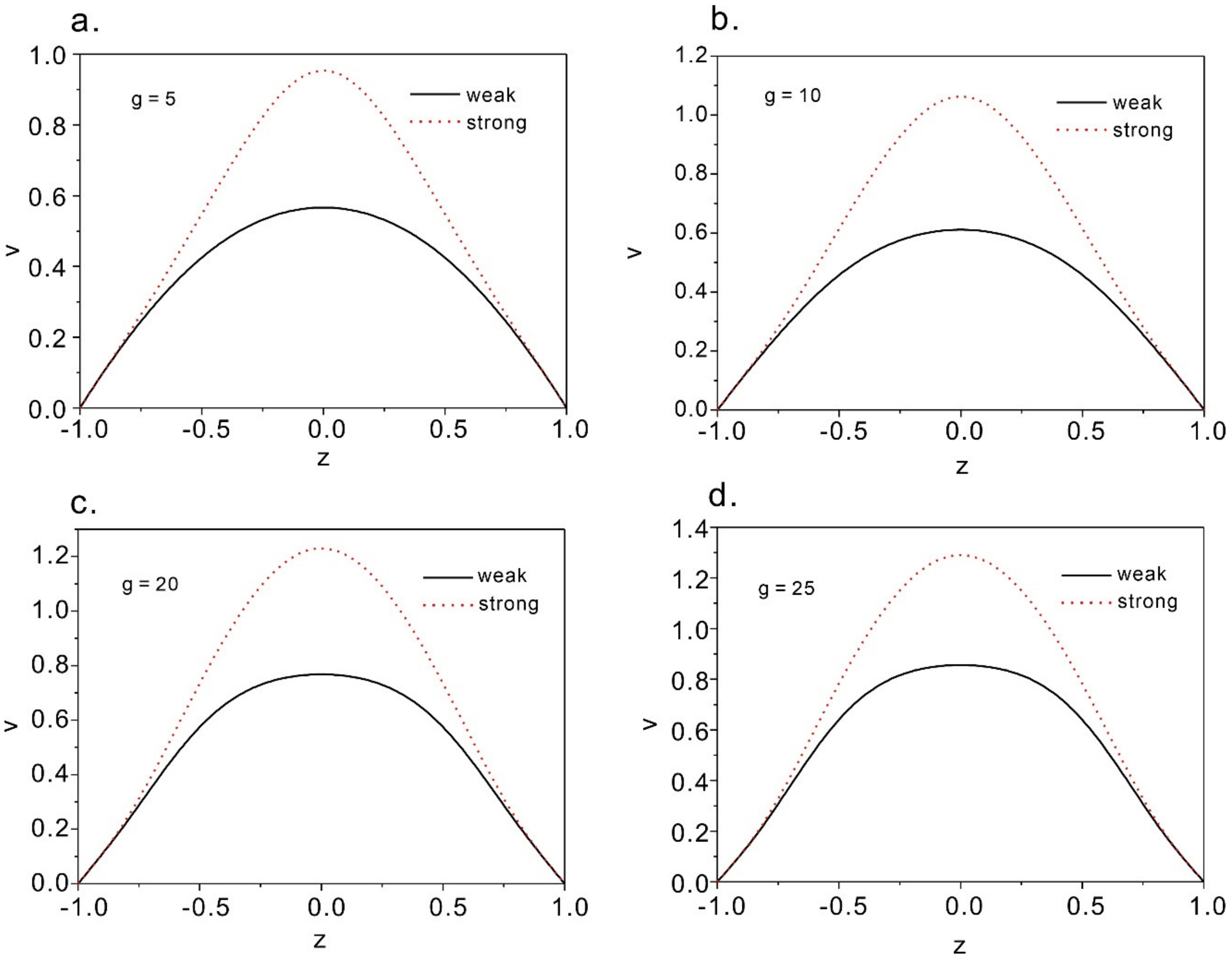
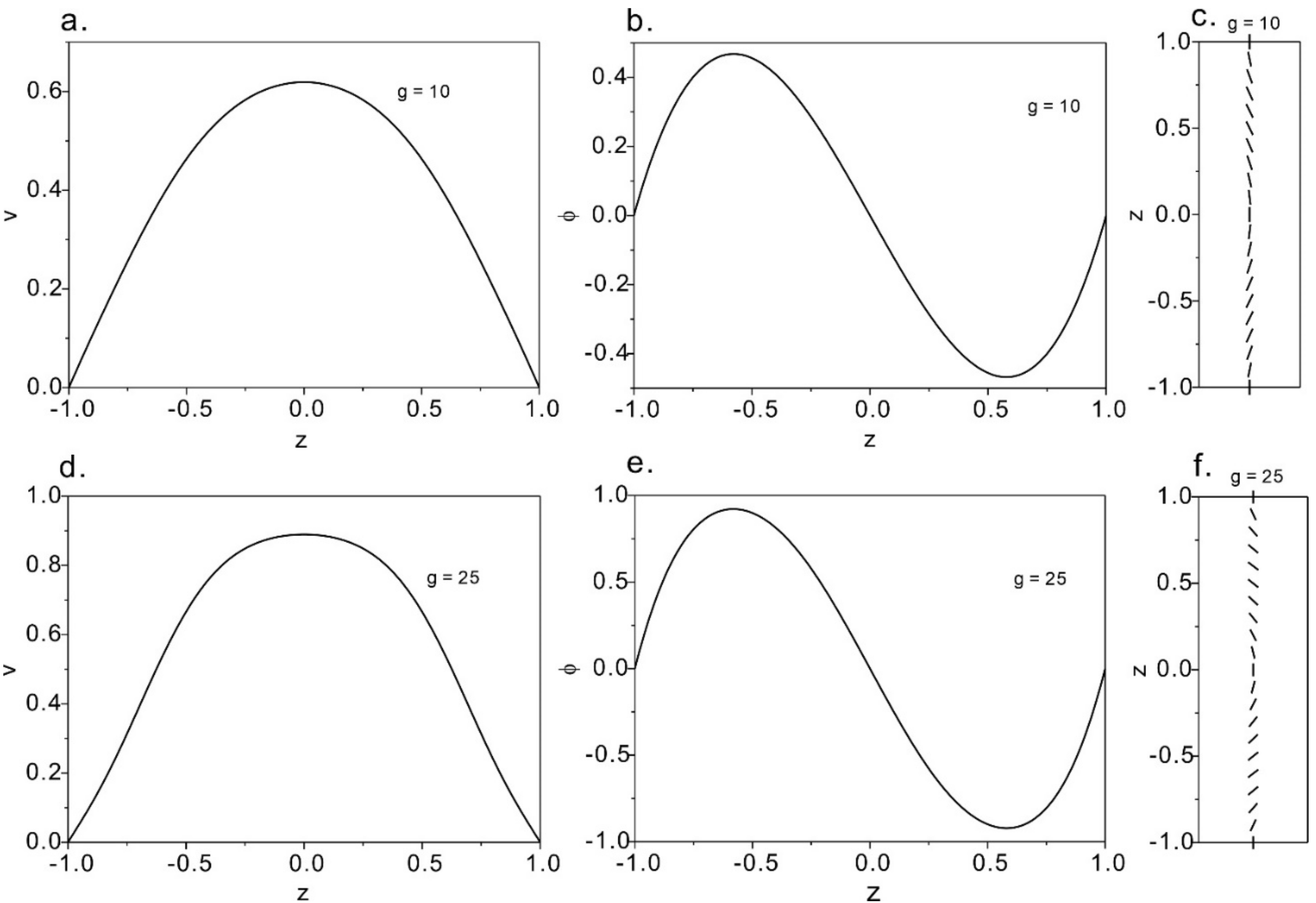
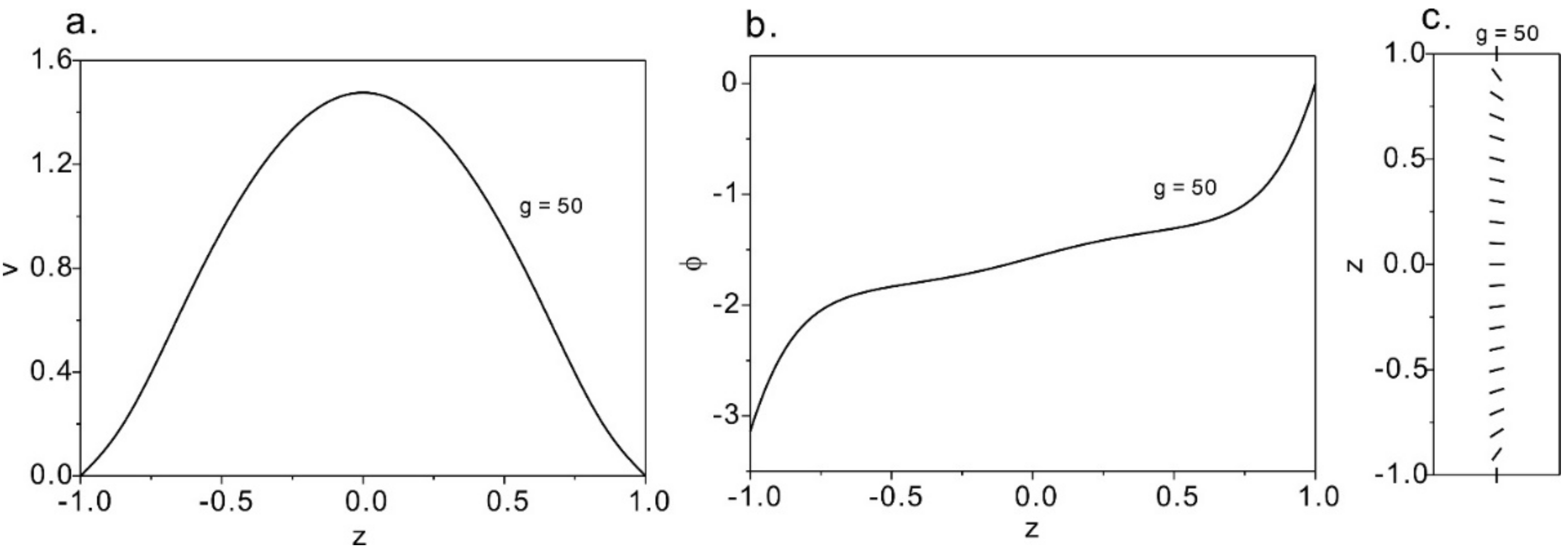
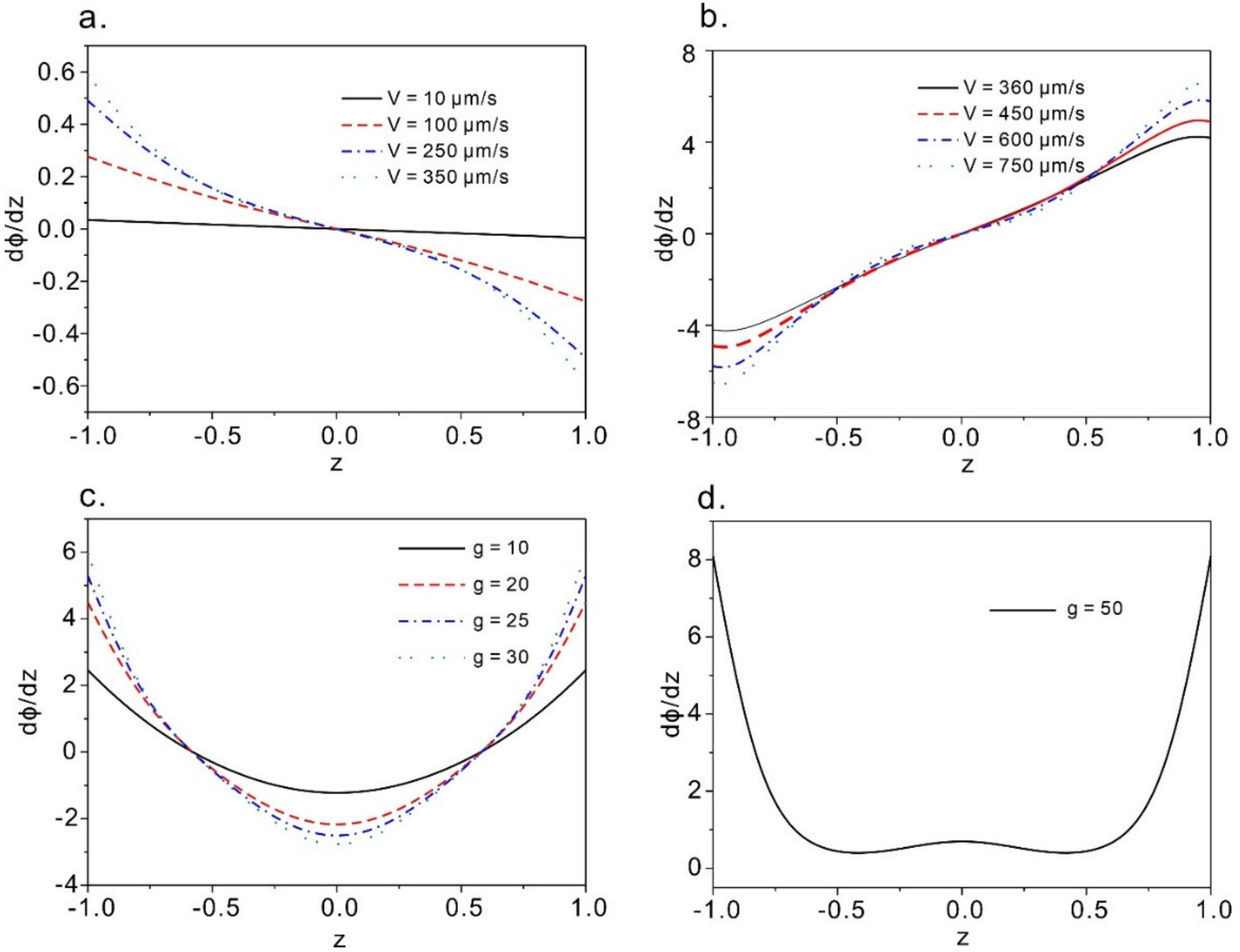
3.2. Poiseuille Flow

Figure 5 shows the solutions at Poiseuille flow with the change of dimensionless pressure gradient g. It can be found that for both weak flow and strong flow anchoring boundary conditions the solutions exist for all flow rates (Figure 5). From T.G. Anderson’s founding on the elastic energies of the two solutions, there is a critical dimensional pressure gradient g*. The energy is lower when the value of g is lower. Therefore, it explains that for cases of g < g*, the weak flow would occur, while for the cases of g > g* the strong flow solution would be expected. In this part, g* is around 40 for strong anchoring boundary condition.

Figure 6 shows weak flow solution at g = 10 and g = 25. We find out that the solution to the anchoring-dominated case has two regions symmetrically placed around the channel centerline. Near the walls and at the centerline, the director follows the strong homeotropic anchoring condition. The velocity profiles are approximately parabolic. The greater the dimensionless pressure gradient is, the greater the velocity and the perturbation of the director are.

Strong flow solutions at g = 50 are plotted in Figure 7, where we see more complex phenomena. The velocity front is a sharper parabolic shape and the director profile is also symmetrical. This differs from the weak flow, where the direction filed is mostly aligned with the flow, regulated by the homeotropic anchoring only near the walls. Therefore, when the pressure gradient further increases, the nematic profile evolves into a flow-aligned state where the director field is majorly flow-aligned. For weak flow, the director orientates normally to the flow orientation at the center w while for strong flow, the director aligns along the flow direction at the center region.

Above, we discussed two kinds of boundary conditions. However, during numerical investigations, a third occurrence may happen, arising from the boundary condition$\Phi \left(-1\right)=\pi$ instead of the condition$\Phi \left(-1\right)=-\pi$. The boundary conditions drive the director to rotate through an angle +$\pi$ across the channel, but the flow near the wall pushes the director in the opposite direction.

4. Discussion

We have calculated the derivative of the directional profile with respect to the channel positions, which represents the sensitivity of the proposed method for flow measurement, as shown in Figure 8. The results indicate that for both the Couette flow and Poiseuille flow, the maximum sensitivity always occurs near the wall boundary (that is the two plates), where the traditionally adopted tracing particle-based measurement technique (namely particle image velocimetry) shows vulnerability. In the cases of Couette flow, we can always find the highest sensitivities near the two plates (see Figure 8a,b) and the lowest sensitivity in the middle region. Similarly, we obtained the maximum sensitivities near the two boundaries (Figure 8c,d). However, when it is under the relatively weak pressure gradient for Poiseuille flow (g = 10~30), Figure 8c indicates a good sensitivity can be obtained in the middle region while for a strong flow case (Figure 8d) g = 50), we get a similar conclusion with scenario in (a) and (b) that the method fails to sense the flow in the center region. Overall, in all of the cases, the region near the boundary favors the measurement sensitivity hence offering the privilege over conventional particle based measurement method. We do believe the no slip boundary condition and the homeotropic anchoring condition near the boundary contribute to the large direct field gradient and hence the relatively high sensitivity.

5. Conclusions

In this paper, we have numerically studied director field and velocity field of two-dimensional Poiseuille flow and Couette flow. The director profile was calculated for various pressure gradient and shear stress. By solving simplified nondimensional L-E equations we obtained numerical results of pressure-driven flow and shear-driven flow.

Firstly, for pressure-driven flow, we find that (i) Limited by weak flow effects, flow alignment does not occur and the director orientation is influenced predominantly by the boundary conditions. In such cases, the velocity profile is like a parabola and symmetric about z = 0. (ii) When the pressure gradient arrives at a value, a qualitative change in the director profile is given explicitly.

Flow alignment occurs and orientational boundary layers exist near the planes. For shear-driven flow, (i) the results show that if the velocity is less or equal to the threshold, the director field is similar to a parabola and the velocity field is presented in a linear manner and the mid-plane angles ${\varnothing }_m$ tend to ${\varnothing }_c$ = arctan[(α₃/α₂)^0.5] with the increasing velocity. (ii) When the velocity exceeds the threshold, the profiles will lose its stability. Vthreshold is about 10⁻³–10⁻⁴ m/s (depend on different parameters). If the velocity exceeds the threshold, the director deviates from the plane of shear. The deformation takes a form of director rotation about the axis perpendicular to the layer plane. As a result, transverse flow arises. The method of nondimensionalizing and the numerical approach proposed in this article will be a potential technique in liquid crystal research. The coupling influence what we analyze is might be able to give clues to the flow dynamics.

Flow measurement by means of the LC reorientation has been proposed recently and in this article, we have theoretically analyzed the viability of such method in flow sensing. The results show that the proposed method has great advantages for sensing near the boundaries which could complement to the technique currently adopted. In this article, we also showed that the orientation angle of the LC follows a non-linear relationship to the flow field distribution. The mathematical model proposed here could be of great potentials when the quantitatively measurement strategy is to be developed for practical applications.

References

1. Leslie, F.M. Some constitutive equations for liquid crystals. Arch. Ration. Mech. Anal. 1968, 28, 265–283. [Google Scholar] [CrossRef]
2. Lubensky, T.C. Molecular Description of Nematic Liquid Crystals. Phys. Rev. A 1970, 2, 2497–2514. [Google Scholar] [CrossRef]
3. Gleeson, J.T.; Palffy-Muhoray, P.; Van Saarloos, W. Propagation of excitations induced by shear flow in nematic liquid crystals. Phys. Rev. A 1991, 44, 2588. [Google Scholar] [CrossRef] [PubMed] [Green Version]
4. Anderson, T.; Mema, E.; Kondic, L.; Cummings, L. Transitions in Poiseuille flow of nematic liquid crystal. International. J. Non-Linear Mech. 2015, 75, 15–21. [Google Scholar] [CrossRef] [Green Version]
5. Sengupta, A.; Tkalec, U.; Ravnik, M.; Yeomans, J.M.; Bahr, C.; Herminghaus, S. Liquid crystal microfluidics for tunable flow shaping. Phys. Rev. Lett. 2013, 110, 048303. [Google Scholar] [CrossRef] [PubMed]
6. Kralj, S.; Žumer, S.; Allender, D.W. Nematic-isotropic phase transition in a liquid-crystal droplet. Phys. Rev. A 1991, 43, 2943–2952. [Google Scholar] [CrossRef] [PubMed] [Green Version]
7. Kralj, S.; Žumer, S.; Allender, D.W. Regular structures in 5CB liquid crystals under the joint action of ac and dc voltages. Phys. Rev. E Stat. Nonlinear Soft Matter Phys. 2012, 85, 3446–3456. [Google Scholar]
8. Bondar, V.G.; Lavrentovich, D.; Pergamenshchik, V.M. Threshold of structural hedgehog-ring transition indrops of a nematic in an alternating electric field. Sov. Phys. JETP 1992, 74, 60–67. [Google Scholar]
9. De Oliveira, B.F.; Avelino, P.P.; Moraes, F.; Oliveira, J.C.R.E. Nematic liquid crystal dynamics under applied electric fields. Phys. Rev. E Stat. Non-Linear Soft Matter Phys. 2010, 82, 041707. [Google Scholar] [CrossRef] [Green Version]
10. Radhakrishnan, M.R.; Matham, V.; Nguyen, N.T. Conoscopic analysis of electric field driven planar aligned nematic liquid crystal. Appl. Opt. 2014, 53, 2773. [Google Scholar]
11. Zhao, Y.; Wang, R.; Yang, C. Interdroplet freezing wave propagation of condensation frosting on micropillar patterned superhydrophobic surfaces of varying pitches. Int. J. Heat Mass Transf. 2017, 108, 1048–1056. [Google Scholar] [CrossRef]
12. Giomi, L.; Kos, Žiga; Ravnik, M.; Sengupta, A. Cross-talk between topological defects in different fields revealed by nematic microfluidics. Proc. Natl. Acad. Sci. USA 2017, 114, 5771–5777. [Google Scholar] [CrossRef] [Green Version]
13. Emeršič, T.; Zhang, R.; Kos, Žiga; Čopar, S.; Osterman, N.; De Pablo, J.J.; Tkalec, U. Sculpting stable structures in pure liquids. Sci. Adv. 2019, 5, eaav4283. [Google Scholar]
14. Fert, A.; Reyren, N.; Cros, V. Magnetic skyrmions: Advances in physics and potential applications. Nat. Rev. Mater. 2017, 2, 17031. [Google Scholar] [CrossRef]
15. Fert, A.; Reyren, N.; Cros, V. Interface-induced phenomena in magnetism. Rev. Mod. Phys. 2017, 89, 025006. [Google Scholar]
16. Berry, J.; Brangwynne, C.P.; Haataja, M. Physical principles of intracellular organization via active and passive phase transitions. Rep. Prog. Phys. 2018, 81, 046601. [Google Scholar] [CrossRef] [Green Version]
17. Pieranski, P.; Godinho, M.H. Flexo-electricity of the dowser texture. Soft Matter 2019, 15, 1469–1480. [Google Scholar] [CrossRef]
18. Pieranski, P.; Godinho, M.H. Curvature elasticity of smectic-C liquid crystals and formation of stripe domains along thickness gradients in menisci of free-standing films. Phys. Rev. E 2020, 101, 032701. [Google Scholar]
19. Huber, L.; Suzuki, R.; Krüger, T.; Frey, E.; Bausch, A.R. Emergence of coexisting ordered states in active matter systems. Science 2018, 361, 255–258. [Google Scholar] [CrossRef] [Green Version]
20. Huber, L.; Suzuki, R.; Krüger, T.; Frey, E.; Bausch, A.R. Tunable structure and dynamics of active liquid crystals. Sci. Adv. 2018, 4, eaat7779. [Google Scholar]
21. Leslie, F.M. Theory of Flow Phenomena in Liquid Crystals. Adv. Liquid Cryst. 1979, 4, 1–81. [Google Scholar]
22. Squires, T.M. Microfluidics: Fluid physics at the nanoliter scale. Rev. Mod. Phys. 2005, 77, 977–1026. [Google Scholar] [CrossRef] [Green Version]
23. Batista, V.; Blow, M.L.; Da Gama, M.M.T. The effect of anchoring on the nematic flow in channels. Soft Matter 2015, 11, 4674–4685. [Google Scholar] [CrossRef] [PubMed] [Green Version]
24. Batista, V.; Blow, M.L.; Da Gama, M.M.T. Apparent viscosity during simple shearing flow of nematic liquid crystals. J. Phys. D Appl. Phys. 1977, 10, 1471. [Google Scholar]
25. Currie, P.K.; MacSithigh, G.P. The stability and dissipation of solutions for shearing flow of nematic liquid crystals. Q. J. Mech. Appl. Math. 1979, 32, 499–511. [Google Scholar] [CrossRef]
26. Huang, Y.; Shinoj, V.K.; Wong, T.; Matham, M.V. Particle free optical imaging of flow field by liquid crystal polarization. Opt. Express 2018, 26, 10452. [Google Scholar] [CrossRef]
27. Huang, Y.; Xiao, L.; An, T.; Lim, W.; Wong, T.; Sun, H. Fast Dynamic Visualizations in Microfluidics Enabled by Fluorescent Carbon Nanodots. Small 2017, 13, 1700869. [Google Scholar] [CrossRef]
28. Huang, Y.; Wang, Y.L.; Wong, T.N. AC electric field controlled non-Newtonian filament thinning and droplet formation on the microscale. Lab Chip 2017, 17, 2969. [Google Scholar] [CrossRef]
29. Parodi, O. Stress tensor for a nematic liquid crystal. J. Phys. 1970, 31, 581–584. [Google Scholar] [CrossRef]
30. Stewart, I.W. The Static and Dynamic Continuum Theory of Liquid Crystals; Taylor & Francis: Abingdon, UK, 2004. [Google Scholar]
Figure 1. Schematics and description of the mathematical model of a nematic liquid crystal in the Couette flow. The upper plate is moved to the right at a constant velocity.
Micromachines 12 00028 g001
Figure 2. Schematics and the mathematical description of a nematic liquid crystal in the Poiseuille flow.
Micromachines 12 00028 g002
Figure 3. (a) Weak flow director profile across the dimensionless channel width −1≤ z ≤ 1 under strong anchoring and g = 25 (Anderson, T. G. et al., 2015). (b) The calculated director profile of strong anchoring at g = 25.
Micromachines 12 00028 g003
Figure 4. (a) Director profiles at different velocities of the upper plate. (b) The maximum directional angle at different velocities of the upper plate.
Micromachines 12 00028 g004
Figure 5. Strong and weak flow solutions at different dimensional pressure gradients. (ad) correspond to the condition of g = 5, 10, 20, and 25 respectively.
Micromachines 12 00028 g005
Figure 6. Velocity profiles and director fields at strong anchoring condition. (ac): The solution of strong anchoring at g = 10. (a) Velocity distributions over the channel width; (b) angle of the director; (c) director distributions over the microchannel. (df): Director and flow distributions within the microchannel under the pressure of g = 25.
Micromachines 12 00028 g006
Figure 7. The solution of strong solution at g = 50. (a) The velocity profile; (b) angle of the director; (c) the distribution of the director at g = 50.
Micromachines 12 00028 g007
Figure 8. Positional sensitivity of the directional profile of the LC flow. (a) and (b) are sensitivities of the LC in Couette flow at various velocities of the upper plate; (c) and (d) represent the sensitivities at various dimensional pressure gradient in Poiseuille flow.
Micromachines 12 00028 g008
Publisher’s Note: MDPI stays neutral with regard to jurisdictional claims in published maps and institutional affiliations.