Author Contributions
Conceptualization, D.F., M.R.-C., C.B. and S.C.; methodology, D.F., M.R.-C., C.B. and S.C.; software, D.F.; validation, D.F., M.R.-C., C.B. and S.C.; formal analysis, D.F.; investigation, D.F.; resources, L.B. and S.C.; data curation, D.F.; writing—original draft preparation, D.F. and M.R.-C.; writing—review and editing, D.F., M.R.-C., C.B., L.B. and S.C.; visualization, D.F.; supervision, M.R.-C., C.B., L.B. and S.C.; project administration, L.B. and S.C.; funding acquisition, L.B. and S.C. All authors have read and agreed to the published version of the manuscript. All the reported work, except a few data treatments and the writing of the paper, have been performed at Institut Clément Ader (ICA), Toulouse.
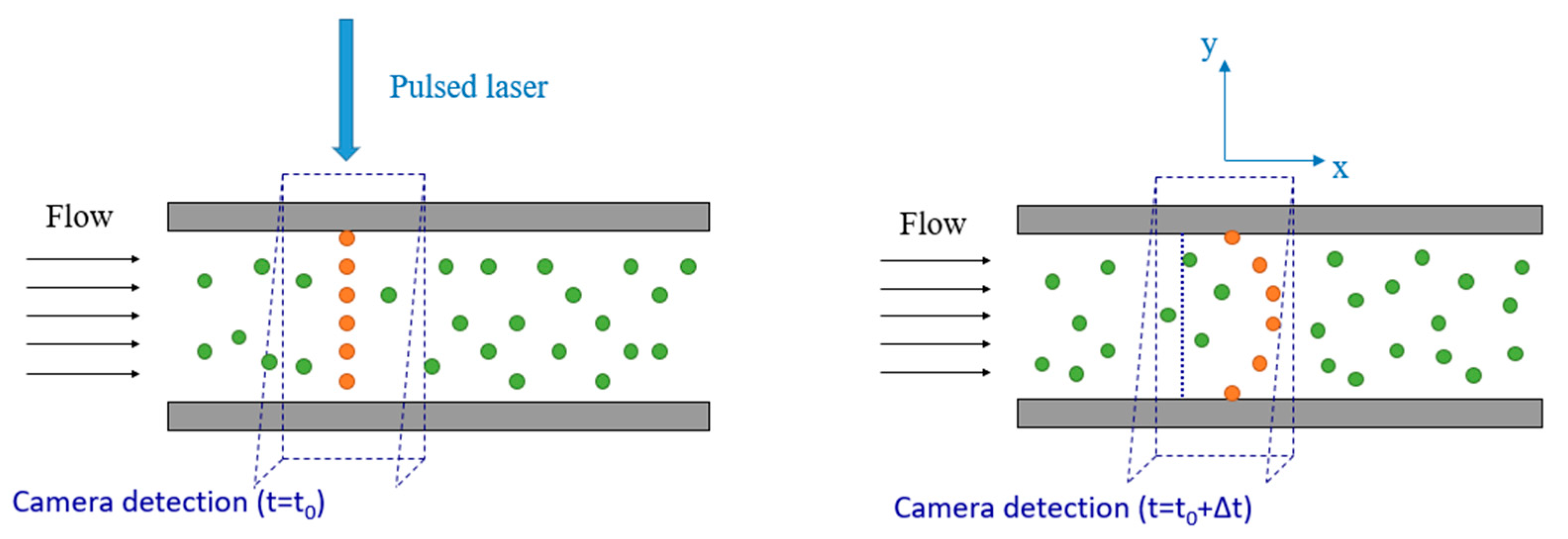
Figure 1.
Basic principle of 1D-molecular tagging velocimetry (MTV) by direct phosphorescence, for a gas flowing in a plane channel from left to right.
Figure 1.
Basic principle of 1D-molecular tagging velocimetry (MTV) by direct phosphorescence, for a gas flowing in a plane channel from left to right.
Figure 2.
Gas system for application of MTV to the gas–vapor mixture flows at low pressures. T1 and T2 are two tanks; P are pressure sensors; V1 is the inlet channel valve; and V2 is the outlet channel valve.
Figure 2.
Gas system for application of MTV to the gas–vapor mixture flows at low pressures. T1 and T2 are two tanks; P are pressure sensors; V1 is the inlet channel valve; and V2 is the outlet channel valve.
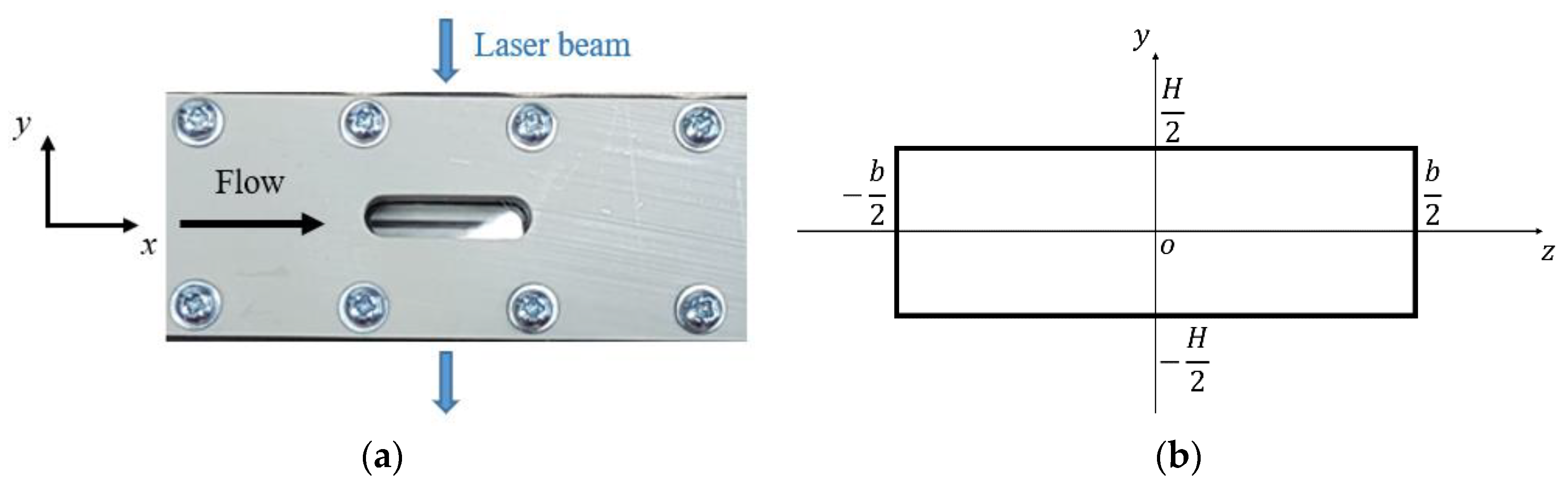
Figure 3.
In (a), a global view of the test section along the channel from the point of the CCD camera. The blue arrows indicate the optical access for the laser beam and the black arrow shows the gas flow direction. In (b), a sketch of the channel cross-section along with the adopted Cartesian coordinate system.
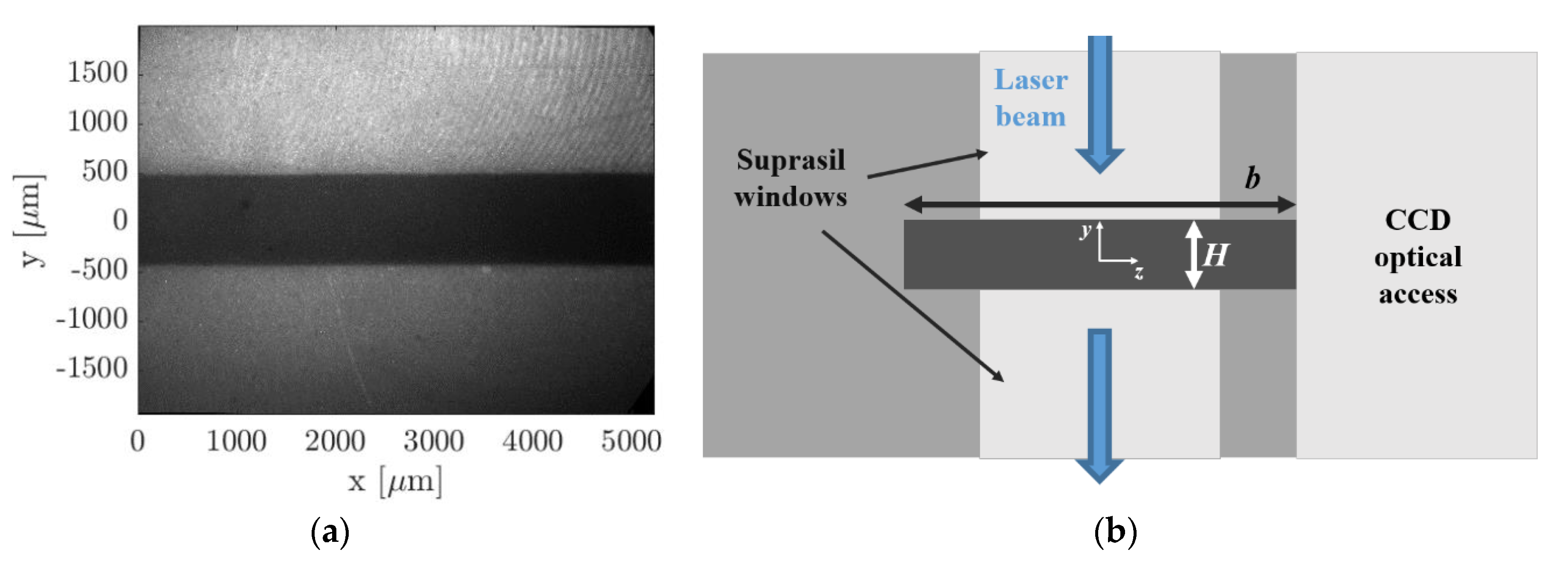
Figure 4.
In (a), an image of the channel gap in the region of interest for MTV, recorded with the CCD. In (b), a sketch of the channel cross-section at the MTV test section. The upper and lower bright regions correspond to the Suprasil® windows for the laser beam access. The bright region on the right represents the optical access for the CCD camera. The width of the cross-section and the distance between the Suprasil® windows are indicated on the image as and , respectively.
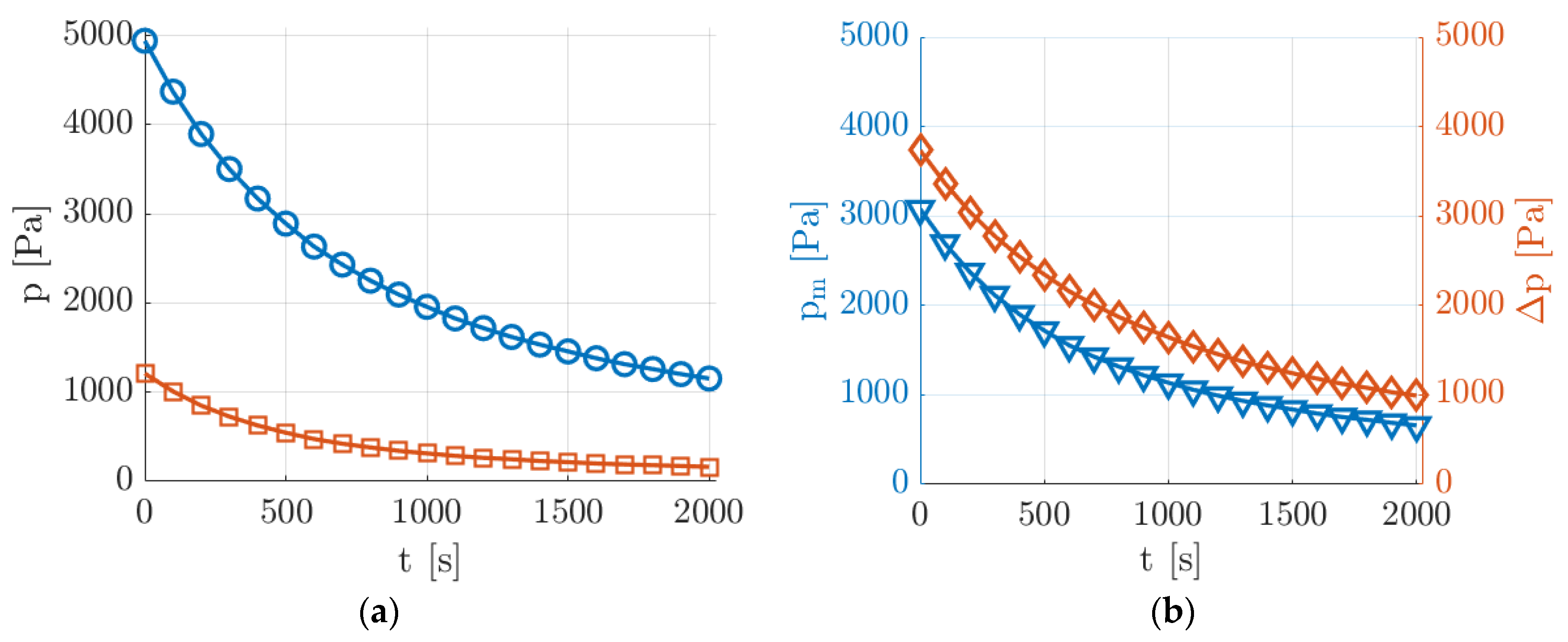
Figure 5.
Evolution in time of the experimental pressure conditions generated at low pressures acquired by pressure sensors P1 and P2: (a) upstream (O) and downstream (☐) pressure measurements and (b) mean pressure (▽) and pressure difference (◇).
Figure 5.
Evolution in time of the experimental pressure conditions generated at low pressures acquired by pressure sensors P1 and P2: (a) upstream (O) and downstream (☐) pressure measurements and (b) mean pressure (▽) and pressure difference (◇).
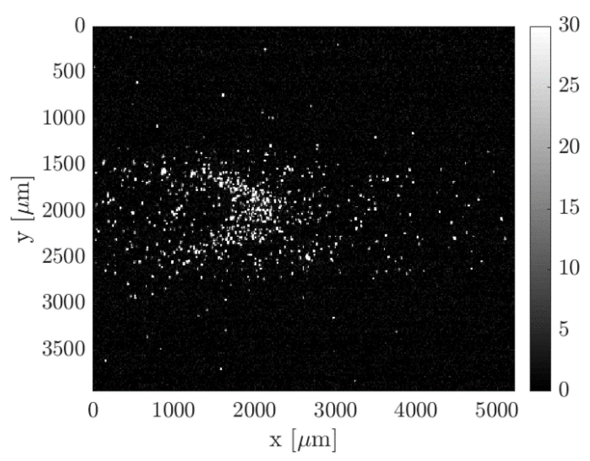
Figure 6.
Example of a raw image acquisition of the acetone emission in argon flow at = 30 kPa, = 550 Pa, and an acetone molar concentration = 20%. The image results from the integration of = 100 laser excitations, with delay = 50 µs, gain 100%, IRO gate 100 ns, and 4 × 4 binning.
Figure 6.
Example of a raw image acquisition of the acetone emission in argon flow at = 30 kPa, = 550 Pa, and an acetone molar concentration = 20%. The image results from the integration of = 100 laser excitations, with delay = 50 µs, gain 100%, IRO gate 100 ns, and 4 × 4 binning.
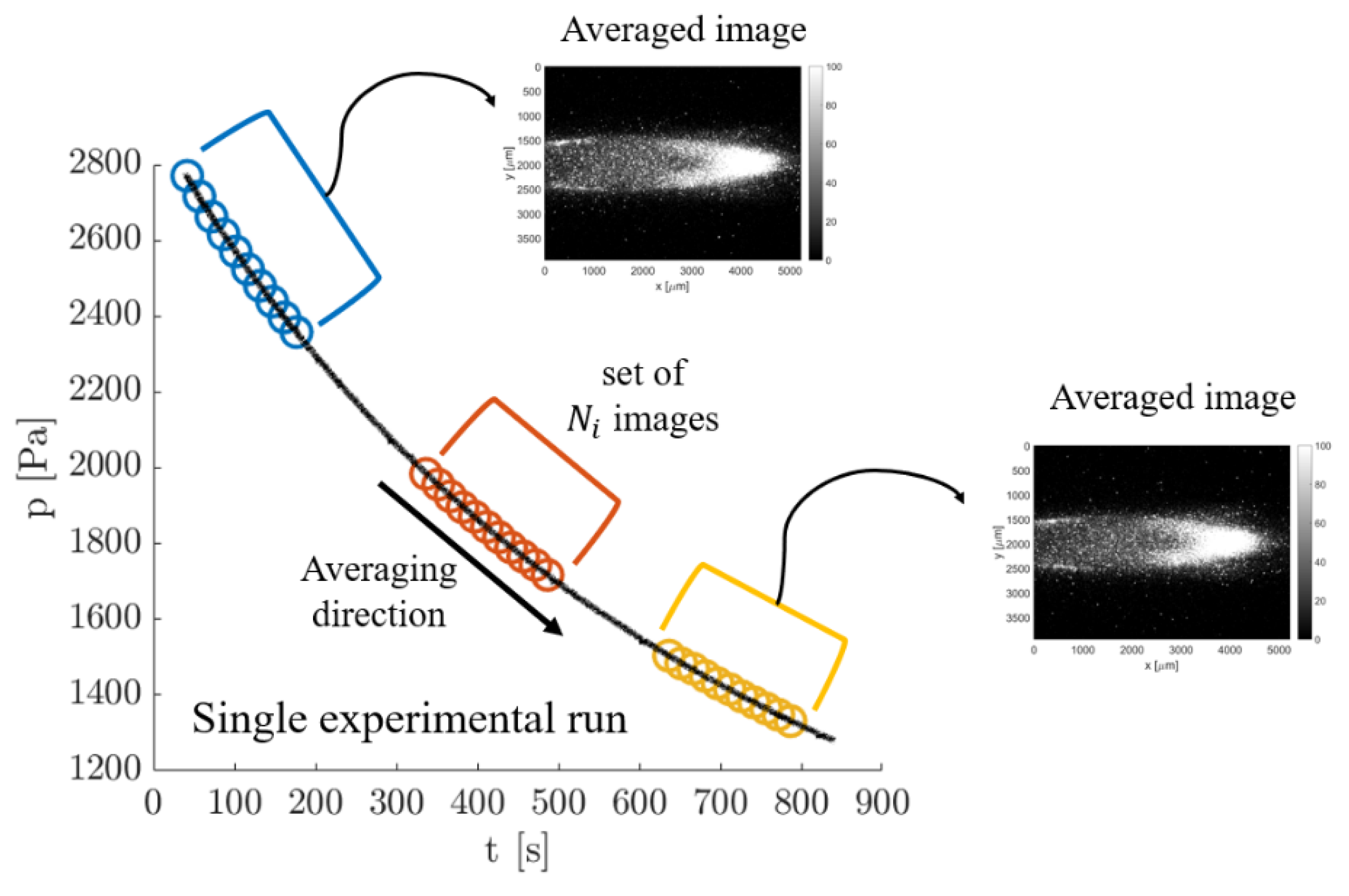
Figure 7.
Qualitative illustration of the strategy used for producing an averaged image from a group of images. The average is made “in cascade” on images recorded during the same experimental run.
Figure 7.
Qualitative illustration of the strategy used for producing an averaged image from a group of images. The average is made “in cascade” on images recorded during the same experimental run.
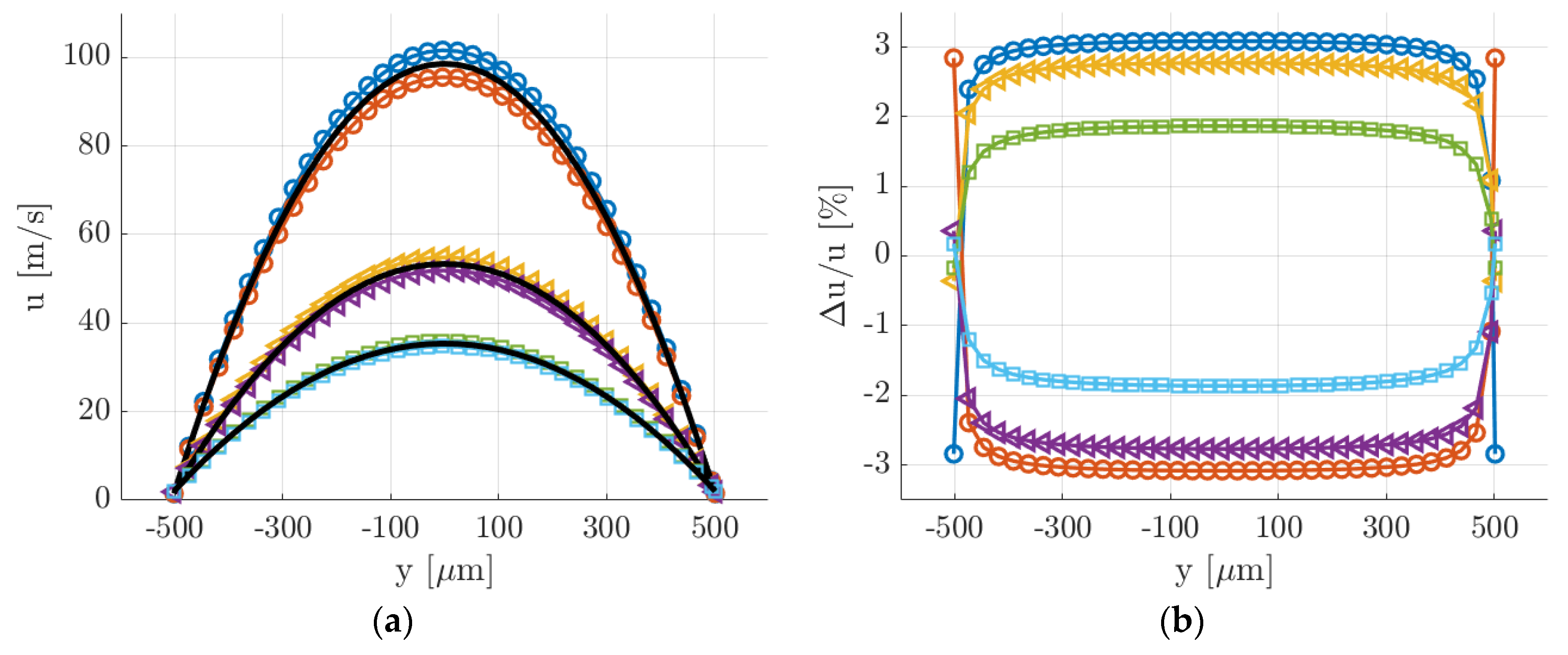
Figure 8.
(a) Analytical velocity profiles at = 100 s (O), 1000 s (◁), and 2000 s (☐) during the experimental run. The evolution of during the recording of = 20 consecutive images is illustrated. At each time , the figure reports: the velocity profile captured by the first image of the group; the velocity profile captured by the last image of the group; the average velocity profile (solid black lines) that the image resulting from the average of the images would represent. (b) Relative variation of the velocity profile with respect to the average velocity profile at = 100 s (O), 1000 s (◁), and 2000 s (☐).
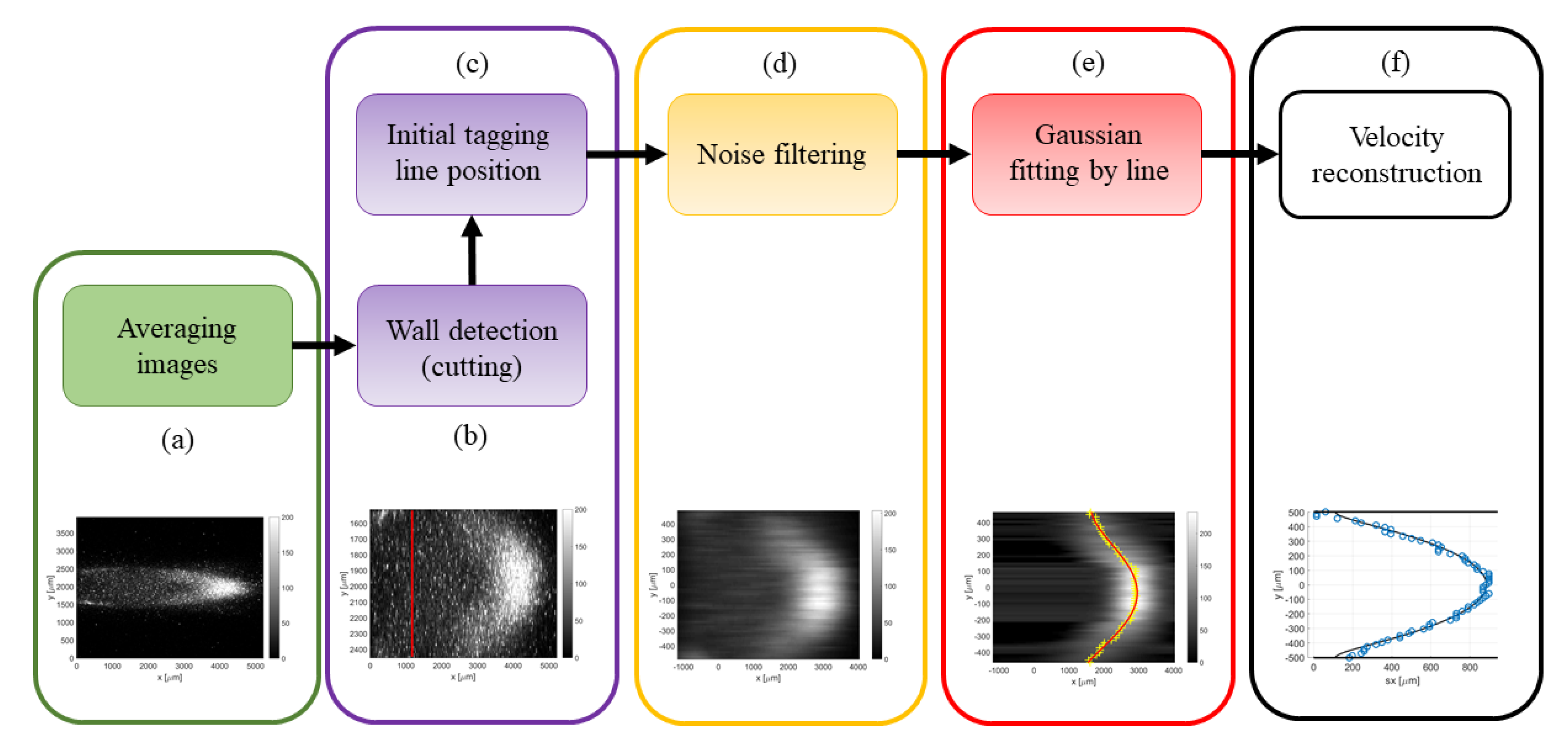
Figure 9.
Flow chart of the image post-processing: (a) image averaging; (b) detecting wall position and image cutting; (c) detecting tagged line position; (d) filtering background noise; (e) Gaussian fitting per each horizontal line of pixels; and (f) velocity reconstruction from the displacement data .
Figure 10.
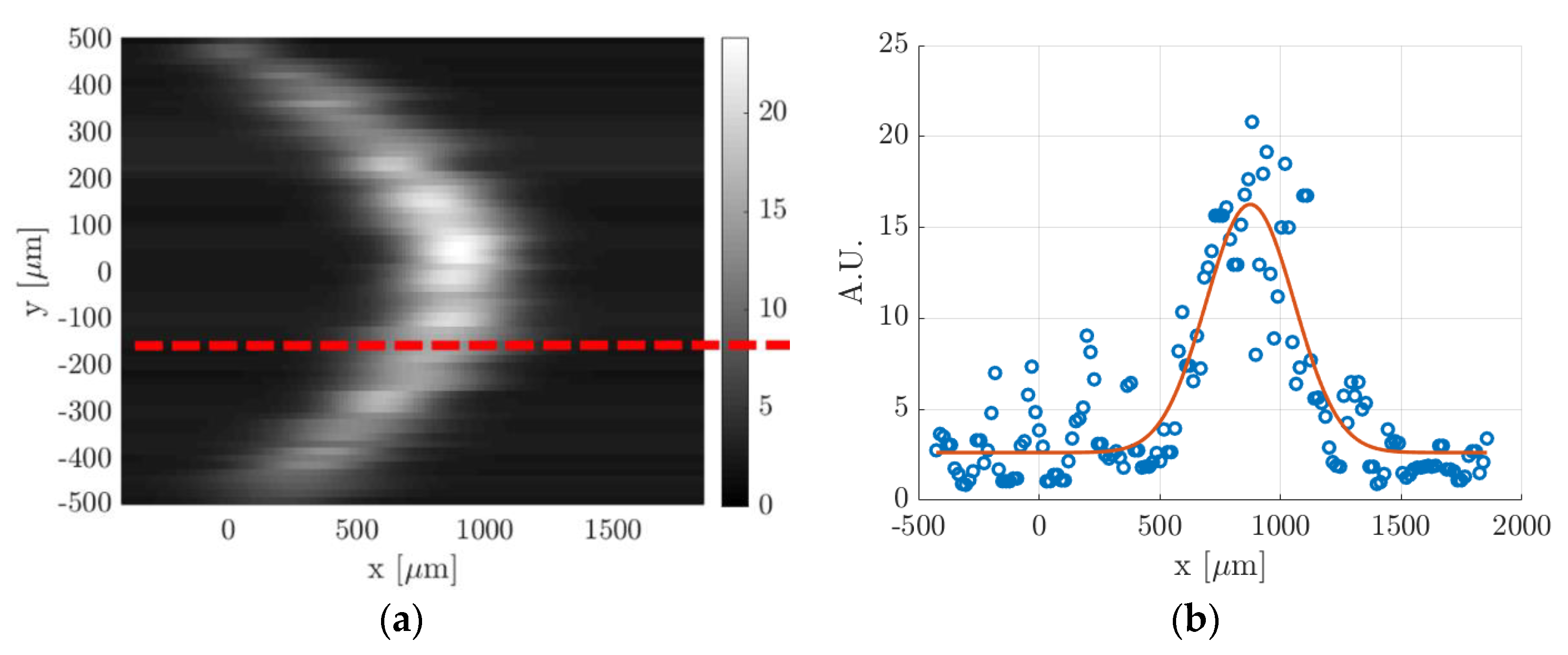
Post-processing procedure for detecting the initial position of the tagged line: (a) raw image of acetone early emission and (b) fitting of the maximum intensity along the y-coordinate detected in the region of interest.
Figure 10.
Post-processing procedure for detecting the initial position of the tagged line: (a) raw image of acetone early emission and (b) fitting of the maximum intensity along the y-coordinate detected in the region of interest.
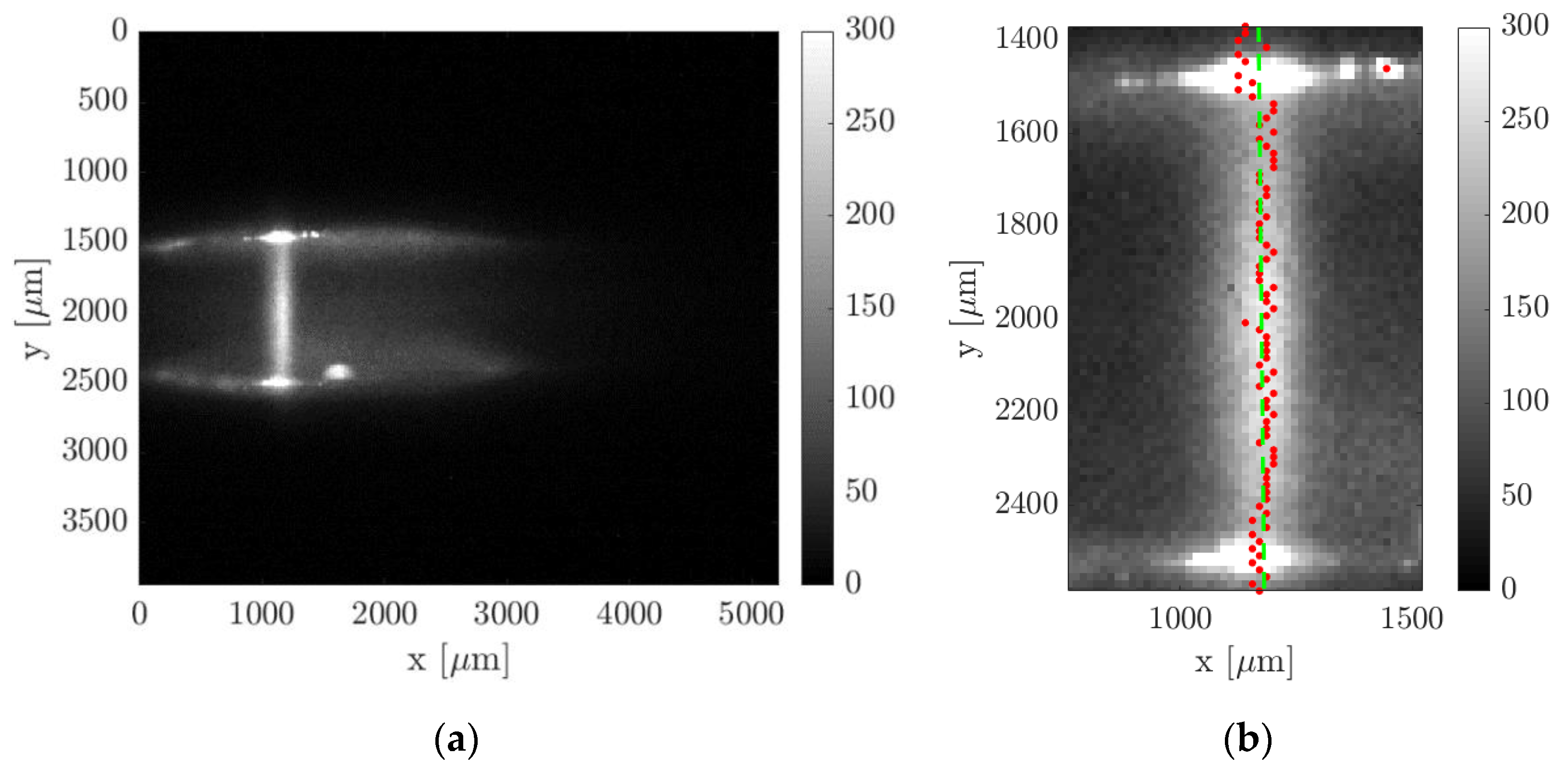
Figure 11.
(a) Image resulting from the application of the Gaussian fitting per line to a raw MTV image and (b) example of data distribution along a horizontal line of pixels, indicated by the red dashed line in (a), and the corresponding Gaussian fitting (A.U. stands for arbitrary unit).
Figure 11.
(a) Image resulting from the application of the Gaussian fitting per line to a raw MTV image and (b) example of data distribution along a horizontal line of pixels, indicated by the red dashed line in (a), and the corresponding Gaussian fitting (A.U. stands for arbitrary unit).
Figure 12.
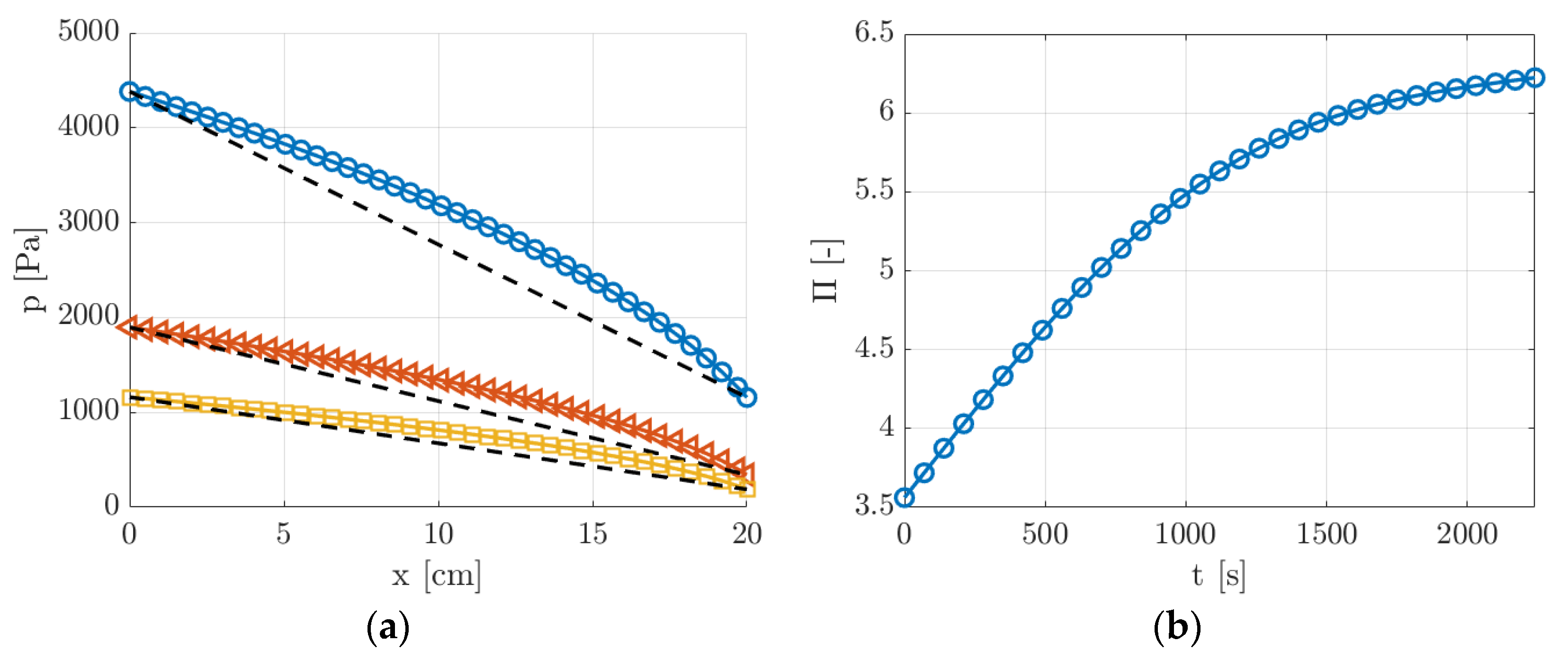
(a) Pressure distribution along the channel length at three different times = 100, 1000, and 2000 s during the experimental run, which correspond to pressure ratios = 3.8 (O), 5.5 (◁), and 6.2 (☐). The dashed lines represent the linear pressure distributions when rarefaction and compressibility effects are neglected; (b) time evolution of pressure ratio during the experimental run.
Figure 12.
(a) Pressure distribution along the channel length at three different times = 100, 1000, and 2000 s during the experimental run, which correspond to pressure ratios = 3.8 (O), 5.5 (◁), and 6.2 (☐). The dashed lines represent the linear pressure distributions when rarefaction and compressibility effects are neglected; (b) time evolution of pressure ratio during the experimental run.
Figure 13.
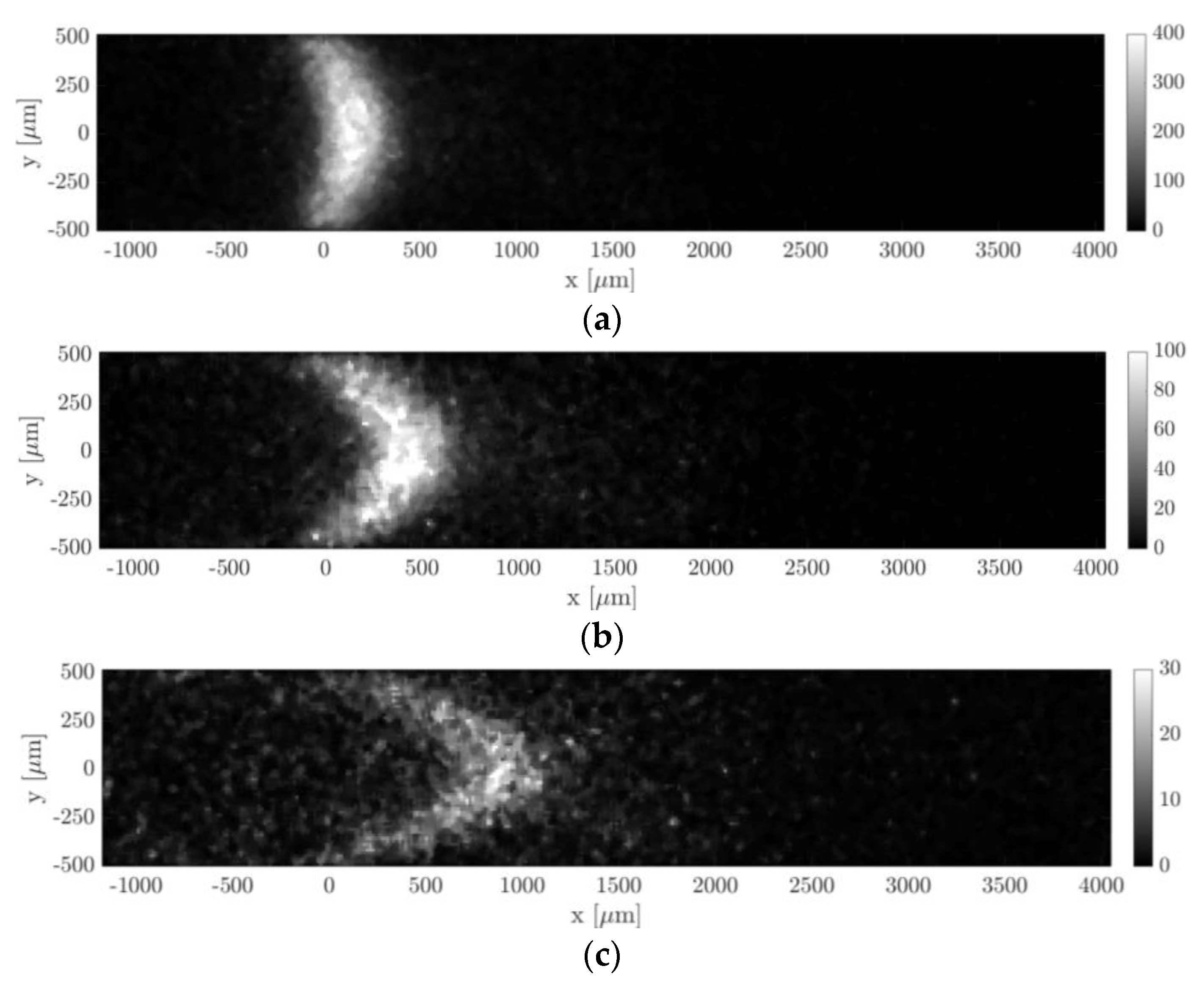
MTV acquisitions of argon–acetone flow with = 20%: (a) = 10 µs, = 27.38 kPa, and = 528.4 Pa; (b) = 25 µs, = 28.83 kPa, and = 538.8 Pa; and (c) = 50 µs, = 30.36 kPa, and = 549.9 Pa. The recording parameters are = 100, = 20, = 100%, and = 100 ns. The acquisitions are made with a 4 × 4 binning. The laser pulse energy was varying between 30 and 40 µJ.
Figure 13.
MTV acquisitions of argon–acetone flow with = 20%: (a) = 10 µs, = 27.38 kPa, and = 528.4 Pa; (b) = 25 µs, = 28.83 kPa, and = 538.8 Pa; and (c) = 50 µs, = 30.36 kPa, and = 549.9 Pa. The recording parameters are = 100, = 20, = 100%, and = 100 ns. The acquisitions are made with a 4 × 4 binning. The laser pulse energy was varying between 30 and 40 µJ.
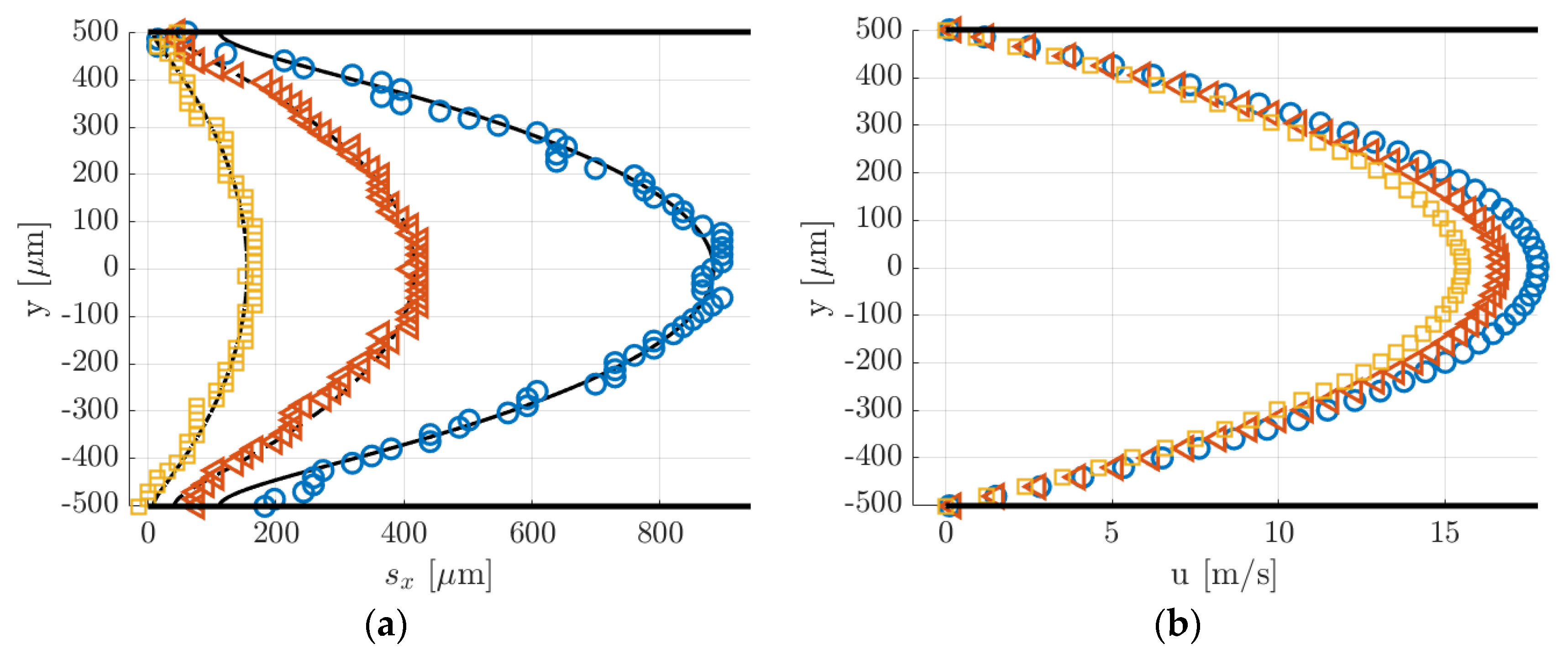
Figure 14.
(
a) Displacement data computed by applying the Gaussian fitting per line to the images of
Figure 13. The black lines represent the numerical solutions for the displacement profile provided by the reconstruction method; (
b) velocity reconstruction from the displacement data in (
a):
= 10 µs (
☐), 25 µs (◁), and 50 µs (O).
Figure 15.
MTV acquisitions of argon–acetone flow with = 20%: (a) = 20 µs, = 6904 Pa, and = 371 Pa; (b) = 30 µs, = 6620 Pa, and = 367 Pa; (c) = 40 µs, = 6337 Pa, and = 362.8 Pa; and (d) = 50 µs, = 6071 Pa, and = 358.6 Pa. The recording parameters are: = 100, = 20, = 100%, and = 100 ns. The acquisitions are made with a 4 × 4 binning. The laser pulse energy was varying between 20 and 30 µJ.
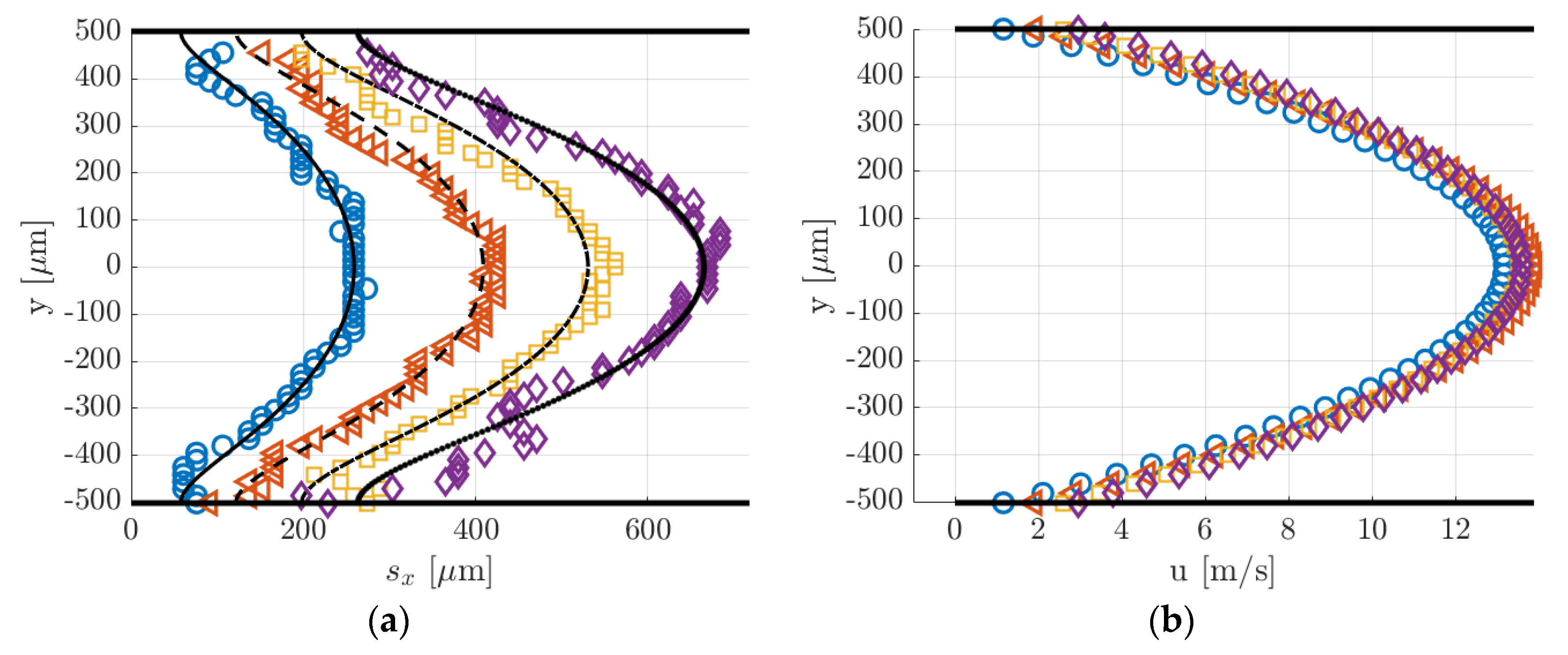
Figure 16.
(
a) Displacement data computed by applying the Gaussian fitting per line to the images of
Figure 15. The black lines represent the numerical solutions for the displacement profile provided by the reconstruction method; (
b) velocity reconstruction from the displacement data in (
a):
= 20 µs (O), 30 µs (◁), 40 µs (
☐), and 50 µs (
◇).
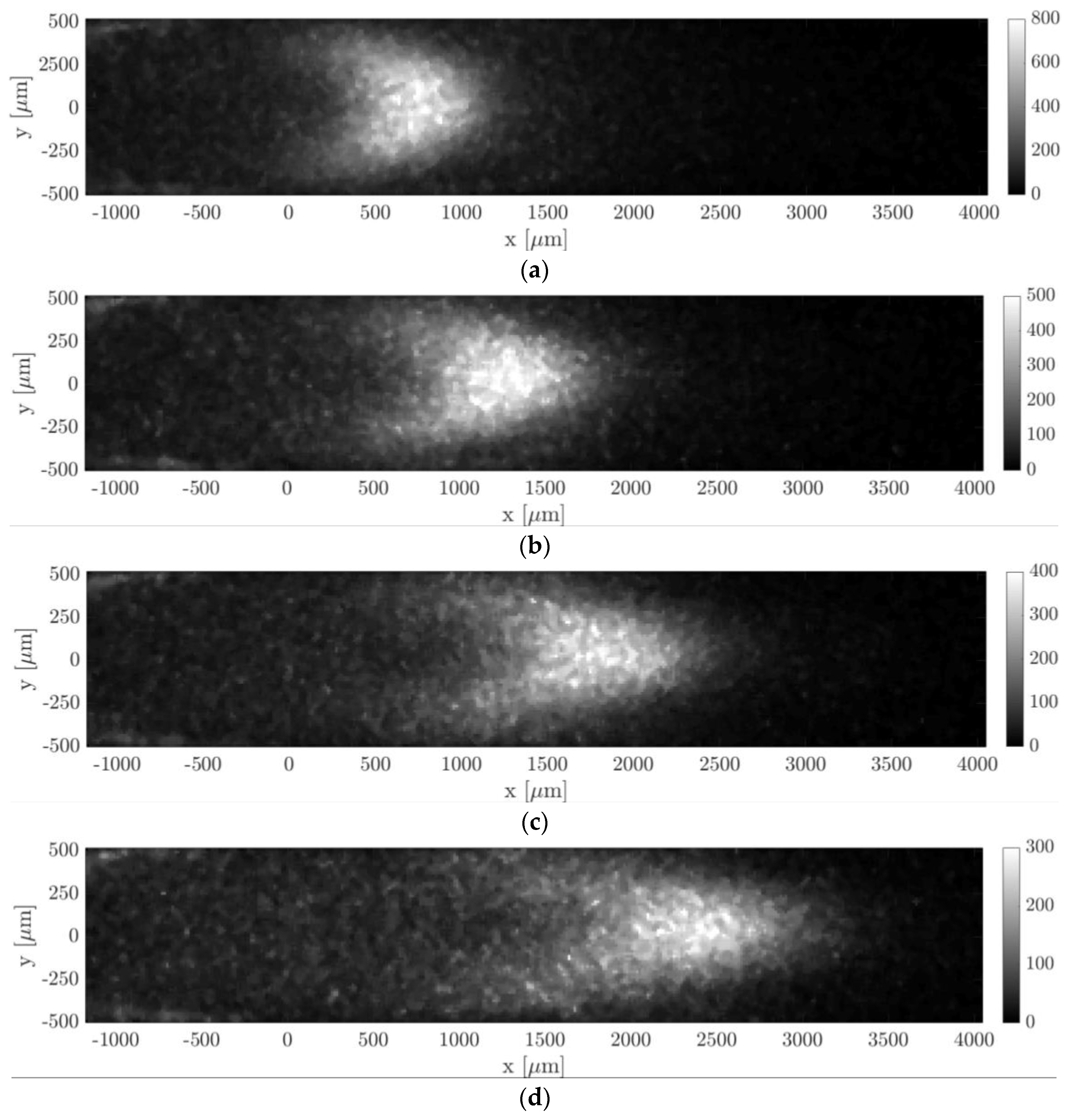
Figure 17.
MTV acquisitions of helium–acetone flow with = 20%: (a) = 20 µs, = 1576 Pa, and = 1789.2 Pa; (b) = 30 µs, = 1580 Pa, and = 1793.2 Pa; (c) = 40 µs, = 1576.6 Pa, and = 1789.2 Pa; and (d) = 50 µs, = 1578.7 Pa, and = 1791.8 Pa. The recording parameters used are: = 100, = 20, = 100%, and = 500 ns. The acquisitions are made with a 4 × 4 binning. The laser pulse energy was varying between 80 and 120 µJ.
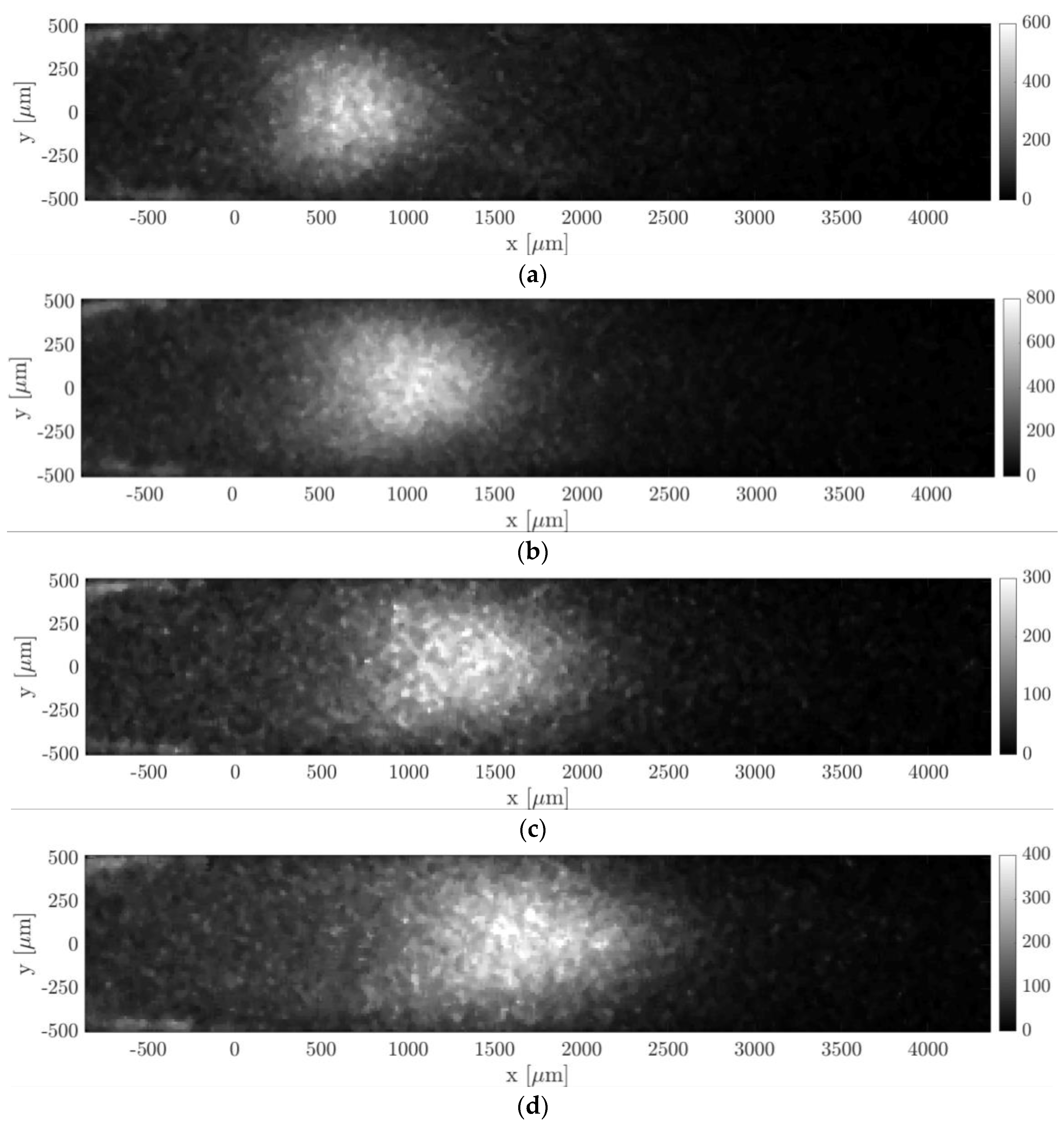
Figure 18.
MTV acquisitions of helium–acetone flow with = 20%: (a) = 20 µs, 500 ns, = 920 Pa, and = 1092.7 Pa; (b) = 30 µs, = 1000 ns, = 920.3 Pa, and = 1093.4 Pa; (c) = 40 µs, = 500 ns, = 919.1 Pa, and = 1091.8 Pa; and (d) = 50 µs, = 1000 ns, = 919.1 Pa, and = 1090.7 Pa. The recording parameters used are: = 100, = 20, and = 100%. The acquisitions are made with a 4 × 4 binning. The laser pulse energy was varying between 80 and 100 µJ.
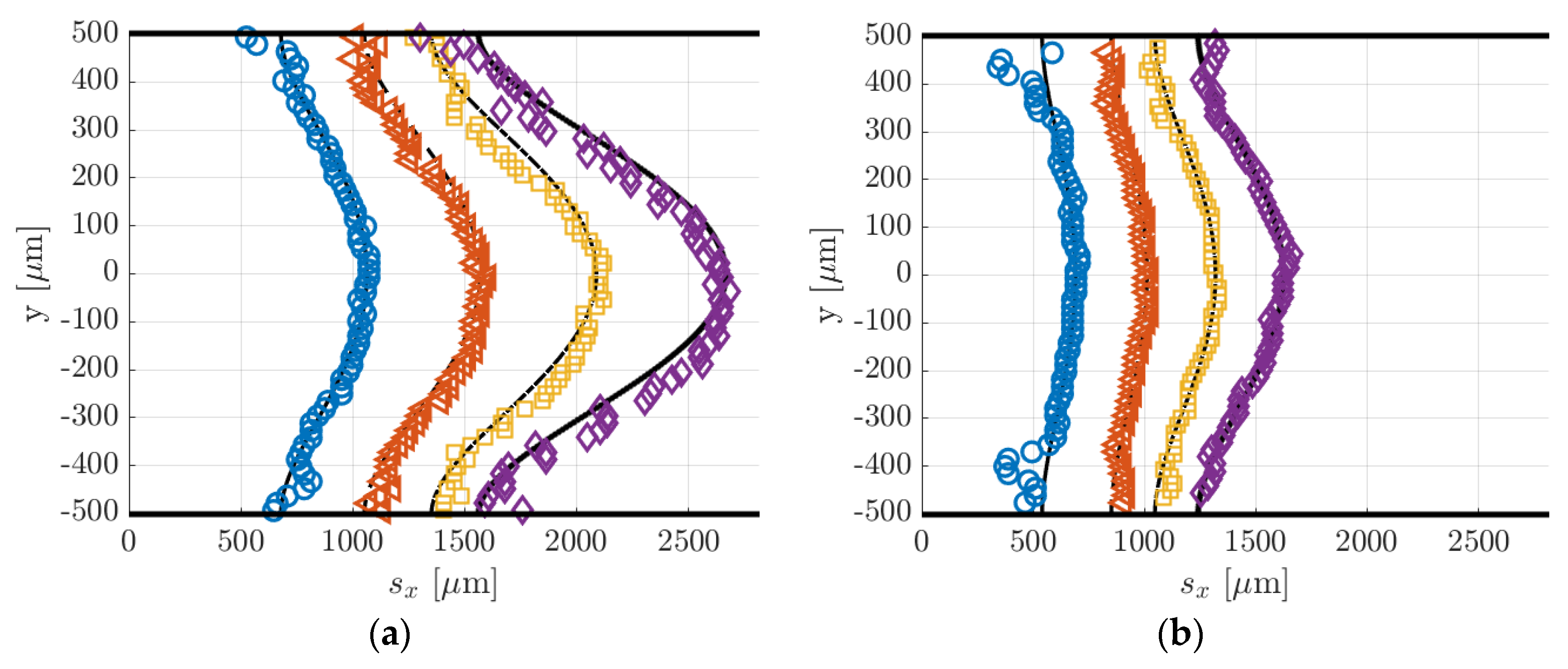
Figure 19.
(
a) Displacement data computed by applying the Gaussian fitting per line to the MTV images at (
a)
= 1580 Pa (
Figure 17) and (
b)
= 920 Pa (
Figure 18):
= 20 µs (O), 30 µs (◁), 40 µs (
☐), and 50 µs (
◇). The black lines represent the numerical solutions for the displacement profile provided by the reconstruction method. The two figures are on the same spatial scale.
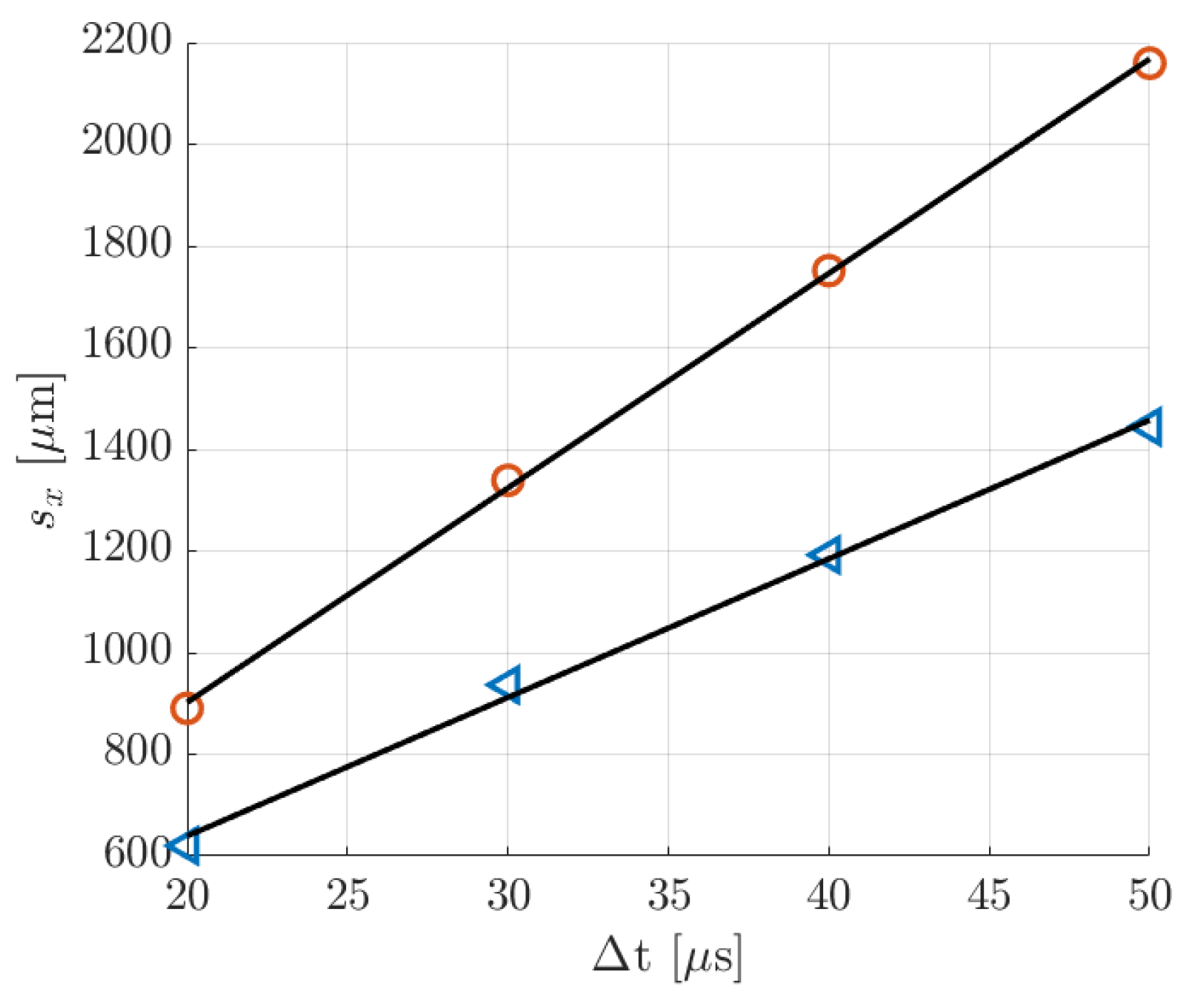
Figure 20.
Mean molecular displacement in helium flow at delays = 20, 30, 40, and 50 µs: (O) data at 1.6 kPa; (◁) data at 920 Pa. The black solid line represents the linear interpolation of the MTV data, which provides an average velocity = 42.2 m/s for the data at 1.6 kPa and = 27.28 m/s for the data at 920 Pa.
Table 1.
Flow properties associated to the images of
Figure 13. The reported percentage change indicates how much the properties vary inside the group of
= 20 averaged images.
Table 1.
Flow properties associated to the images of
Figure 13. The reported percentage change indicates how much the properties vary inside the group of
= 20 averaged images.
| Image | (µs) | (kPa) | (Pa) | (kg/s) | (–) | (–) |
|---|
| Figure 13a | 10 | 27.38 ± 1.5% | 528.4 ± 0.6% | 2.63 × 10⁻⁵ ± 1.6% | 0.039 ± 0.15% | 1.85 × 10⁻⁴ ± 1.5% |
| Figure 13b | 25 | 28.83 ± 1.5% | 538.8 ± 0.6% | 2.79 × 10⁻⁵ ± 1.6% | 0.039 ± 0.15% | 1.75 × 10⁻⁴ ± 1.5% |
| Figure 13c | 50 | 30.36 ± 1.5% | 549.9 ± 0.6% | 2.95 × 10⁻⁵ ± 1.6% | 0.039 ± 0.15% | 1.66 × 10⁻⁴ ± 1.5% |
Table 2.
Flow properties associated to the images of
Figure 15. The reported percentage change indicates how much the properties vary inside the group of
= 20 average images.
Table 2.
Flow properties associated to the images of
Figure 15. The reported percentage change indicates how much the properties vary inside the group of
= 20 average images.
| Image | (µs) | (Pa) | (Pa) | (kg/s) | (–) | (–) |
|---|
| Figure 15a | 20 | 6904 ± 1.2% | 371 ± 0.3% | 5.4 × 10⁻⁶ ± 1.5% | 0.032 ± 0.27% | 7.3 × 10⁻⁴ ± 1.2% |
| Figure 15b | 30 | 6620 ± 1.2% | 367 ± 0.31% | 5.2 × 10⁻⁶ ± 1.5% | 0.031 ± 0.29% | 7.3 × 10⁻⁴ ± 1.2% |
| Figure 15c | 40 | 6337 ± 1.2% | 362.8 ± 0.31% | 4.9 × 10⁻⁶ ± 1.5% | 0.031 ± 0.3% | 8 × 10⁻⁴ ± 1.2% |
| Figure 15d | 50 | 6071 ± 1.2% | 358.6 ± 0.31% | 4.6 × 10⁻⁶ ± 1.5% | 0.031 ± 0.31% | 8.3 × 10⁻⁴ ± 1.2% |
Table 3.
Flow properties associated to the images of
Figure 17. The reported percentage change indicates how much the properties vary inside the group of
= 20 average images.
Table 3.
Flow properties associated to the images of
Figure 17. The reported percentage change indicates how much the properties vary inside the group of
= 20 average images.
| Image | (µs) | (Pa) | (Pa) | (kg/s) | (–) | (–) |
|---|
| Figure 17a | 20 | 1576 ± 3.6% | 1789.2 ± 3.2% | 1.7 × 10⁻⁶ ± 6.5% | 0.07 ± 2.7% | 0.008 ± 3.5% |
| Figure 17b | 30 | 1580 ± 3.6% | 1793.2 ± 3.2% | 1.7 × 10⁻⁶ ± 6.2% | 0.07 ± 2.5% | 0.008 ± 3.5% |
| Figure 17c | 40 | 1576.6 ± 3.6% | 1789.2 ± 3.2% | 1.7 × 10⁻⁶ ± 6.4% | 0.07 ± 2.7% | 0.008 ± 3.5% |
| Figure 17d | 50 | 1578.7 ± 3.6% | 1791.8 ± 3.2% | 1.7 × 10⁻⁶ ± 6% | 0.07 ± 2.2% | 0.008 ± 3.5% |
Table 4.
Flow properties associated to the images of
Figure 18. The reported percentage change indicates how much the properties vary inside the group of
= 20 average images.
Table 4.
Flow properties associated to the images of
Figure 18. The reported percentage change indicates how much the properties vary inside the group of
= 20 average images.
| Image | (µs) | (Pa) | (Pa) | (kg/s) | (–) | (–) |
|---|
| Figure 18a | 20 | 920 ± 2.3% | 1092.7 ± 2.2% | 6.5 × 10⁻⁷ ± 4.4% | 0.045 ± 2% | 0.014 ± 2.3% |
| Figure 18b | 30 | 920.3 ± 2.3% | 1093.4 ± 2.3% | 6.5 × 10⁻⁷ ± 4% | 0.045 ± 1.7% | 0.014 ± 2.3% |
| Figure 18c | 40 | 919.1 ± 2.3% | 1091.8 ± 2.2% | 6.5 × 10⁻⁷ ± 3.9% | 0.045 ± 1.6% | 0.014 ± 2.3% |
| Figure 18d | 50 | 919.1 ± 2.4% | 1090.7 ± 2.2% | 6.5 × 10⁻⁷ ± 4.4% | 0.045 ± 2% | 0.014 ± 2.3% |
Table 5.
Thickness
of the displacement profile related to the data of argon–acetone flow at 6 kPa (
Figure 16a) and of helium–acetone flows at 1.6 kPa (
Figure 18a) and at 920 Pa (
Figure 18b).
Table 5.
Thickness
of the displacement profile related to the data of argon–acetone flow at 6 kPa (
Figure 16a) and of helium–acetone flows at 1.6 kPa (
Figure 18a) and at 920 Pa (
Figure 18b).
| (µs) | Argon–acetone at 6.5 kPa | Helium–acetone at 1.6 kPa | Helium–acetone at 920 Pa |
|---|
| 20 | 206 µm | 384.7 µm | 149.3 µm |
| 30 | 298.3 µm | 528.5 µm | 159.3 µm |
| 40 | 334.96 µm | 748.3 µm | 271.9 µm |
| 50 | 398.35 µm | 1124.98 µm | 380.8 µm |
Table 6.
Average velocities
and
with estimated uncertainties, and relative deviation between
and
calculated for the image data of
Figure 13. The uncertainty range has a confidence level of 95%.
Table 6.
Average velocities
and
with estimated uncertainties, and relative deviation between
and
calculated for the image data of
Figure 13. The uncertainty range has a confidence level of 95%.
| (µs) | (m/s) | (m/s) | (%) |
|---|
| 10 | 12.42 ± 0.74 | 10.47 ± 3 | 18.6 |
| 25 | 12.48 ± 0.74 | 11.21 ± 1.2 | 11.3 |
| 50 | 12.54 ± 0.76 | 11.93 ± 0.6 | 5.1 |
Table 7.
Average velocities
and
with estimated uncertainties, and relative deviation between
and
calculated for the image data of
Figure 15. The uncertainty range has a confidence level of 95%.
Table 7.
Average velocities
and
with estimated uncertainties, and relative deviation between
and
calculated for the image data of
Figure 15. The uncertainty range has a confidence level of 95%.
| (µs) | (m/s) | (m/s) | (%) |
|---|
| 20 | 10.16 ± 0.6 | 9.08 ± 1.52 | 11.9 |
| 30 | 10.06 ± 0.6 | 9.83 ± 0.98 | 2.3 |
| 40 | 9.95 ± 0.6 | 9.92 ± 0.76 | 0.3 |
| 50 | 9.84 ± 0.6 | 9.9 ± 0.6 | 0.6 |
Table 8.
Average velocities
and
with estimated uncertainties, and relative deviation between
and
calculated for the image data of
Figure 17. The uncertainty range has a confidence level of 95%.
Table 8.
Average velocities
and
with estimated uncertainties, and relative deviation between
and
calculated for the image data of
Figure 17. The uncertainty range has a confidence level of 95%.
| (µs) | (m/s) | (m/s) | (%) |
|---|
| 20 | 41.2 ± 2.48 | 44.59 ± 1.52 | 7.6 |
| 30 | 41.35 ± 2.48 | 44.47 ± 0.98 | 7 |
| 40 | 41.28 ± 2.48 | 43.78 ± 0.76 | 5.7 |
| 50 | 41.15 ± 2.46 | 43.09 ± 0.6 | 4.5 |
Table 9.
Average velocities
and
with estimated uncertainties, and relative deviation between
and
calculated for the image data of
Figure 18. The uncertainty range has a confidence level of 95%.
Table 9.
Average velocities
and
with estimated uncertainties, and relative deviation between
and
calculated for the image data of
Figure 18. The uncertainty range has a confidence level of 95%.
| (µs) | (m/s) | (m/s) | (%) |
|---|
| 20 | 26.72 ± 1.6 | 31.06 ± 1.52 | 14 |
| 30 | 26.6 ± 1.6 | 31.24 ± 0.98 | 14.8 |
| 40 | 26.7 ± 1.6 | 29.81 ± 0.76 | 10.4 |
| 50 | 26.77 ± 1.6 | 28.89 ± 0.6 | 7.3 |

 ,
, 


