High-G Calibration Denoising Method for High-G MEMS Accelerometer Based on EMD and Wavelet Threshold


 , ,
, ,  ,
,
Abstract
:1. Introduction
2. Algorithm
2.1. Empirical Mode Decomposition (EMD)
2.2. Wavelet Threshold Denoising
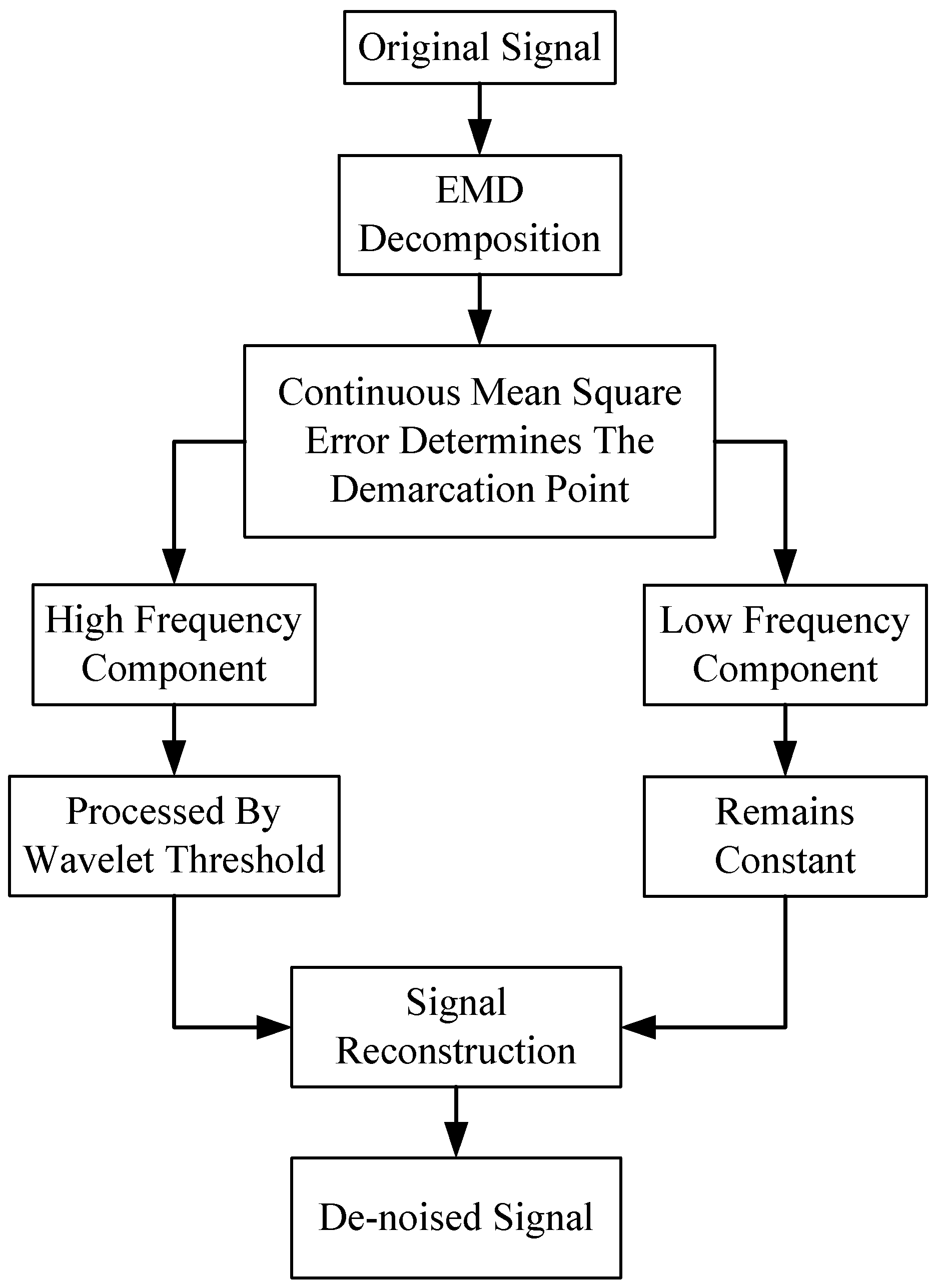
2.3. Wavelet Thresholding Denoising Based on EMD
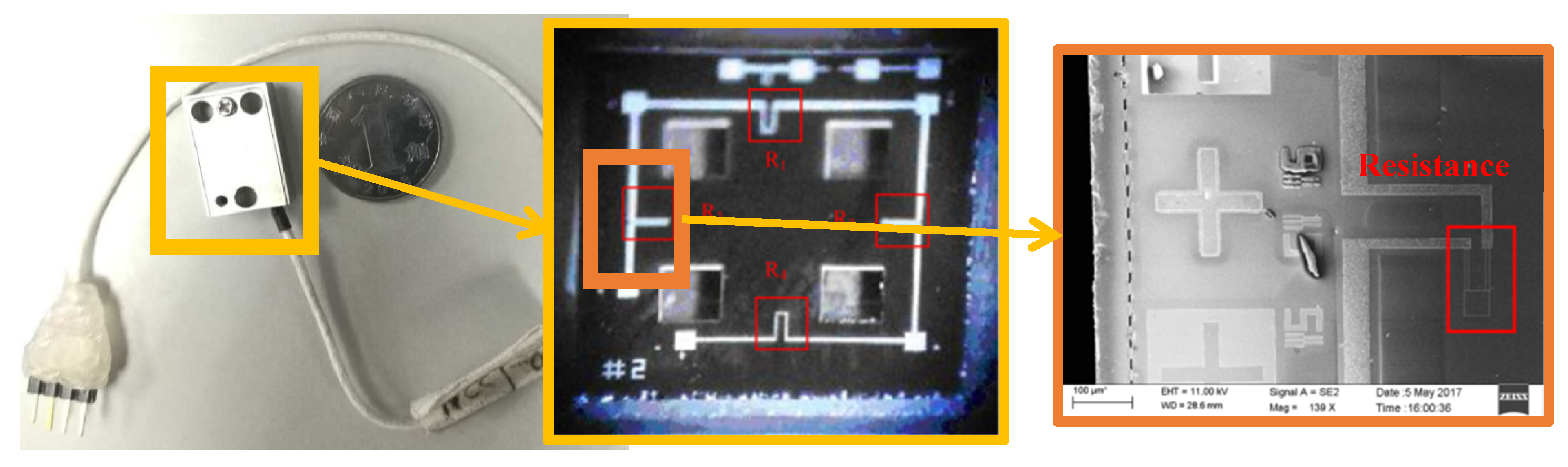
3. High-G MEMS Accelerometer
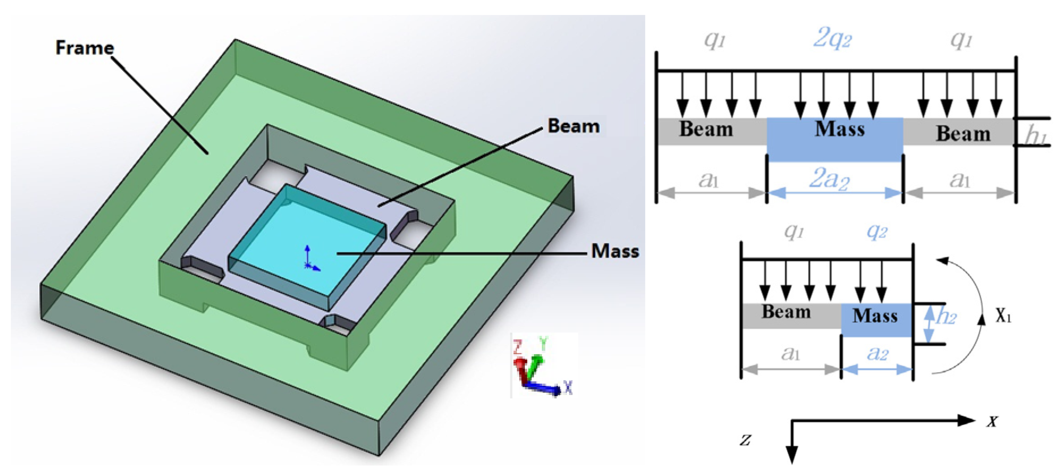
Structure and Structural Parameters of the HGMA
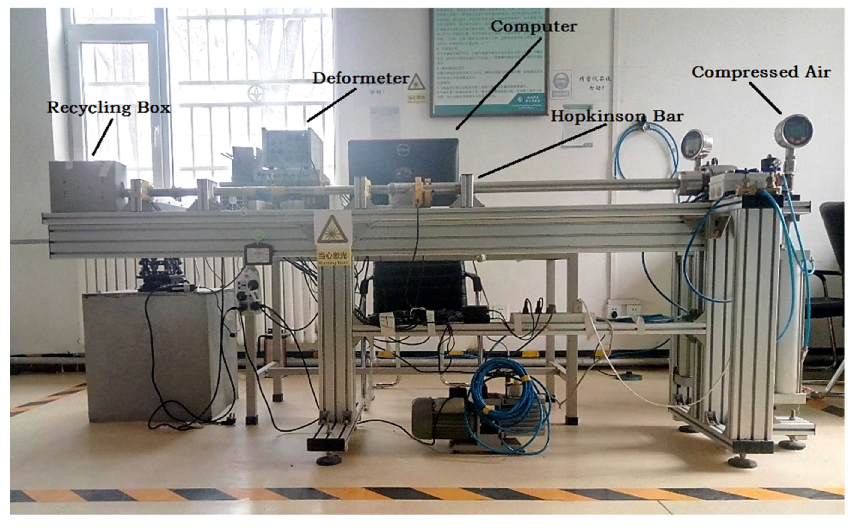
4. Experiment and Verification
4.1. Experiment
4.2. Verification
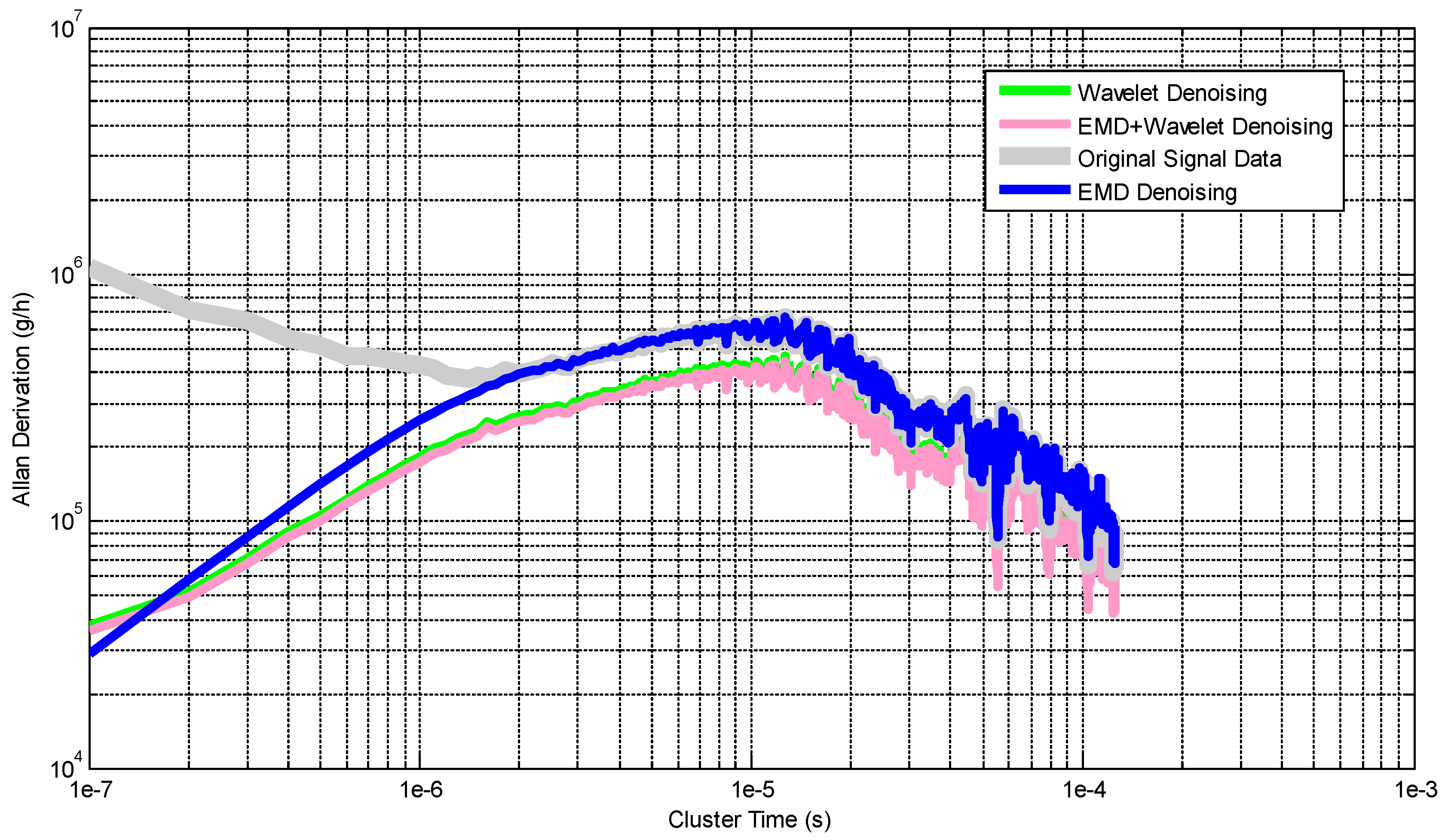
- Preparing stage: before the shock peak, and this part contains the noise signal and the bias characteristic of HGMA. As can be seen from Figure 7, the noise of original signal data is large (peak-peak value is near about 1000 g), and EMD, Wavelet and EMD + Wavelet methods all work well, and which are proved by denoising results.
- Shock stage: the main part of the calibration experiment, the peak value is about 28,030 g, and the pulse wide is about 10 μs. During this stage, the original signal data, EMD and EMD + Wavelet denoising signals almost overlapping, which indicates that these three curves contain the same information. However, the Wavelet denoising signal amplitude is 25,240 g, which is not the real peak value of original signal data, and the error is more than 10%. So, Wavelet method is not suitable for the calibration denoising.
- Vibration stage: after the shock peak, and this part mainly contains HGMA vibration information, which reflects the dynamic characteristic of HGMA. In this stage, it can be seen that the EMD denoising signal occurs distortion phenomenon and cannot reflect the frequency and amplitude information of original data any more. Meanwhile, the amplitude information of original signal data cannot be expressed after Wavelet denoising. Only EMD + Wavelet method follows the original signal data.
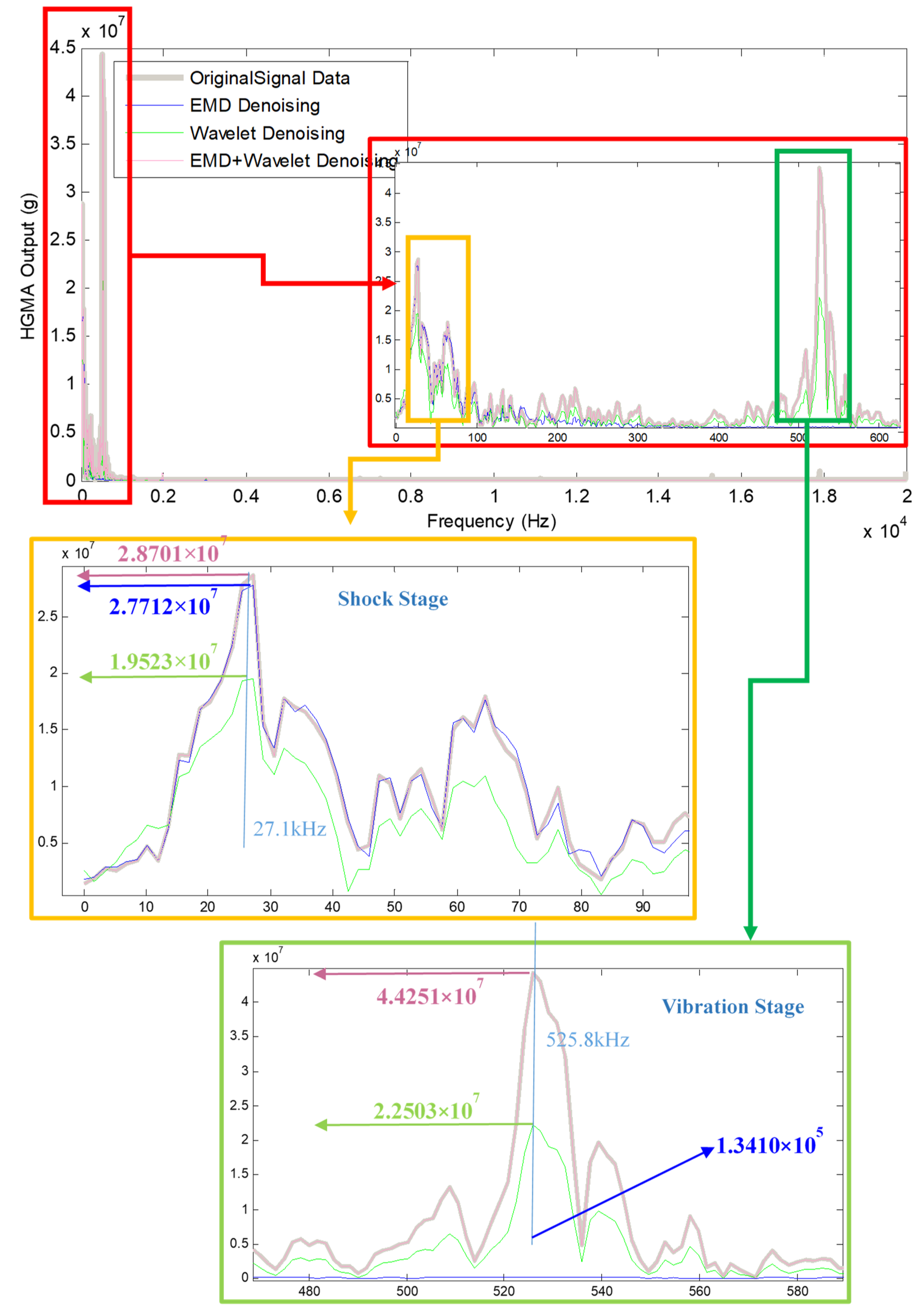
- Shock stage: the frequency peak of this stage is about 27.1 kHz, the original signal data and EMD + Wavelet denoising results have almost the same amplitude and shape (one amplitude is 2.8702 × 10⁷, the other is 2.8701 × 10⁷); the EMD denoising result amplitude is 2.7712 × 10⁷; the Wavelet denoising result amplitude is 1.9523 × 10⁷, which shows that EMD + Wavelet denoising method inherit the real amplitude and frequency information of original signal.
- Vibration stage: the frequency peak of vibration stage is about 525.8 kHz, the original signal data and EMD + Wavelet denoising results have almost the same amplitude and shape (one amplitude is 4.4310 × 10⁷, the other is 4.4251 × 10⁷); the EMD denoising result amplitude is 1.3410 × 10⁵; the Wavelet denoising result amplitude is 2.2503 × 10⁷, which shows that EMD + Wavelet denoising method inherit the real amplitude and frequency information of original signal.
5. Conclusions
Author Contributions
Funding
Conflicts of Interest
References
- Xu, W.; Yang, J.; Xie, G.; Wang, B.; Qu, M.; Wang, X.; Liu, X.; Tang, B. Design and Fabrication of a Slanted-Beam MEMS Accelerometer. Micromachines 2017, 8, 77. [Google Scholar] [CrossRef]
- Mahmood, M.S.; Celik-Butler, Z.; Butler, D.P. Design, fabrication and characterization of flexible MEMS accelerometer using multi-Level UV-LIGA. Sens. Actuators A Phys. 2017, 263, 530–541. [Google Scholar] [CrossRef]
- Baginsky, I.L.; Kostsov, E.G. Capacitive MEMS accelerometers for measuring high-g accelerations. Optoelectronics. Instrum. Data Process. 2017, 53, 294–302. [Google Scholar] [CrossRef]
- Huang, H.; Chen, X.; Zhang, B.; Wang, J. High accuracy navigation information estimation for inertial system using the multi-model EKF fusing adams explicit formula applied to underwater gliders. ISA Trans. 2017, 66, 414–424. [Google Scholar] [CrossRef] [PubMed]
- Cao, H.; Li, H.; Liu, J.; Shi, Y.; Tang, J.; Shen, C. An improved interface and noise analysis of a turning fork microgyroscope structure. Mech. Syst. Signal Process. 2016, 70, 1209–1220. [Google Scholar] [CrossRef]
- Shen, C.; Song, R.; Li, J.; Zhang, X.; Tang, J.; Shi, Y.; Liu, J.; Cao, H. Temperature drift modeling of MEMS gyroscope based on genetic-Elman neural network. Mech. Syst. Signal Process. 2016, 72–73, 897–905. [Google Scholar]
- Cao, H.; Li, H.; Shao, X.; Liu, Z.; Kou, Z.; Shan, Y.; Shi, Y.; Shen, C.; Liu, J. Sensing mode coupling analysis for dual-mass MEMS gyroscope and bandwidth expansion within wide-temperature range. Mech. Syst. Signal Process. 2018, 98, 448–464. [Google Scholar] [CrossRef]
- Cao, H.; Zhang, Y.; Han, Z.; Shao, X.; Gao, J.; Huang, K.; Shi, Y.; Tang, J.; Shen, C.; Liu, J. Pole-Zero-Temperature Compensation Circuit Design and Experiment for Dual-mass MEMS Gyroscope Bandwidth Expansion. IEEE/ASME Trans. Mechatron. 2019. [Google Scholar] [CrossRef]
- Shen, C.; Yang, J.; Tang, J.; Liu, J.; Cao, H. Note: Parallel processing algorithm of temperature and noise error for micro- electro-mechanical system gyroscope based on variational mode decomposition and augmented nonlinear differentiator. Rev. Sci. Instrum. 2018, 89, 076107. [Google Scholar] [CrossRef]
- Cao, H.; Zhang, Y.; Shen, C.; Liu, Y.; Wang, X. Temperature Energy Influence Compensation for MEMS Vibration Gyroscope Based on RBF NN-GA-KF Method. Shock Vib. 2018, 2018, 2830686. [Google Scholar] [CrossRef]
- Huang, Y.Y.; Jing, Y.W.; ShI, Y.B. Non-parametric mobile node localization for IOT by variational Bayesian approximations adaptive Kalman filter. Cogn. Syst. Res. 2018, 52, 27–35. [Google Scholar] [CrossRef]
- Mandal, A.; Niyogi, S. Filter assisted bi-dimensional empirical mode decomposition: A hybrid approach for regional-residual separation of gravity anomaly. J. Appl. Geophys. 2018, 159, 218–227. [Google Scholar] [CrossRef]
- Du, Y.; Du, D. Fault Detection using Empirical Mode Decomposition based PCA and CUSUM with Application to the Tennessee Eastman Process. IFAC PapersOnLine 2018, 51, 488–493. [Google Scholar] [CrossRef]
- Wang, S.T.; Zhao, Z.D. Heart sounds adaptive denoising algorithm based on EMP shreshold. In Intelligent Information Technology Application, Proceedings of the 2010 International Conference on Bio-inspired Systems and Signal Processing (ICBSSP 2010), HongKong, China, 26 October 2010; Curran Associates, Inc.: Red Hook, NY, USA, 2010; pp. 220–223. [Google Scholar]
- Zhang, C. EMD Denoising Method Research Based on HHT. Comput. Knowl. Technol. 2010, 6, 10113–10115. [Google Scholar]
- Zhang, Y. Signal Wavelet Threshold Denoising Research Based on Empirical Mode Decompesition. Ph.D. Thesis, Kunming University of Science and Technology, Kunming, China, June 2011. [Google Scholar]
- Boudraa, A.O.; Cexus, J.C. EMD-based signal filtering. IEEE Trans. Instrum. Meas. 2007, 56, 2196–2202. [Google Scholar] [CrossRef]
- Chen, F. A new approach to signal de-noising based on EMD mode relevance. J. Xihua Univ. Nat. Sci. Ed. 2009, 28, 20–24. [Google Scholar]
- Xu, X.; Luo, M.; Tan, Z.; Pei, R. Echo signal extraction method of laser radar based on improved singular value decomposition and wavelet threshold denoising. Infrared Phys. Technol. 2018, 92, 327–335. [Google Scholar] [CrossRef]
- Bi, F.; Ma, T.; Wang, X. Development of a novel knock characteristic detection method for gasoline engines based on wavelet-denoising and EMD decomposition. Mech. Syst. Signal Process. 2019, 117, 517–536. [Google Scholar] [CrossRef]
- Zhu, B.; Yuan, L.; Ye, S. Examining the multi-timescales of European carbon market with grey relational analysis and empirical mode decomposition. Phys. A Stat. Mech. Appl. 2019, 517, 392–399. [Google Scholar] [CrossRef]
- Schweigmann, M.; Koch, K.P.; Auler, F.; Kirchhoff, F. Improving electrocorticograms of awake and anaesthetized mice using wavelet denoising. Curr. Directions Biomed. Eng. 2018, 4, 469–472. [Google Scholar] [CrossRef]
- Zhang, X. A Modified Artificial Bee Colony Algorithm for Image Denoising Using Parametric Wavelet Thresholding Method. Pattern Recognit. Image Anal. 2018, 28, 557–568. [Google Scholar] [CrossRef]
- Yu, B.; Li, S.; Chen, C.; Xu, J.; Qiu, W.; Wu, X.; Chen, R. Prediction subcellular localization of Gram-negative bacterial proteins by support vector machine using wavelet denoising and Chou’s pseudo amino acid composition. Chemom. Intell. Lab. Syst. 2017, 167, 102–112. [Google Scholar] [CrossRef]
- Guo, Z.; Li, S.; Wang, L.; Tang, Y. Improved alorithm with auto-adaptive threshold for wavelet image denoising. J. Chongqing Univ. Posts Telecommun. Nat. Sci. 2015, 27, 740–744. [Google Scholar]
- Shi, Y.; Yang, Z.; Ma, Z.; Cao, H.; Kou, Z.; Zhi, D.; Chen, Y.; Feng, H.; Liu, J. The Development of a Dual-Warhead Impact System for Dynamic Linearity Measurement of a High-g Micro-Electro-Mechanical-Systems (MEMS) Accelerometer. Sensors 2016, 16, 840. [Google Scholar] [CrossRef]
- Shi, Y.; Zhao, Y.; Feng, H.; Cao, H.; Tang, J.; Li, J.; Zhao, R.; Liu, J. Design, Fabrication and Calibration of a High-G MEMS Accelerometer. Sens. Actuators A Phys. 2018, 279, 733–742. [Google Scholar] [CrossRef]


| Beam | Mass | |||||
|---|---|---|---|---|---|---|
| Parameters | Length (a1) | Width (b1) | Height (c1) | Length (a2) | Width (b2) | Height (c1) |
| Size (μm) | 350 | 800 | 80 | 800 | 800 | 200 |
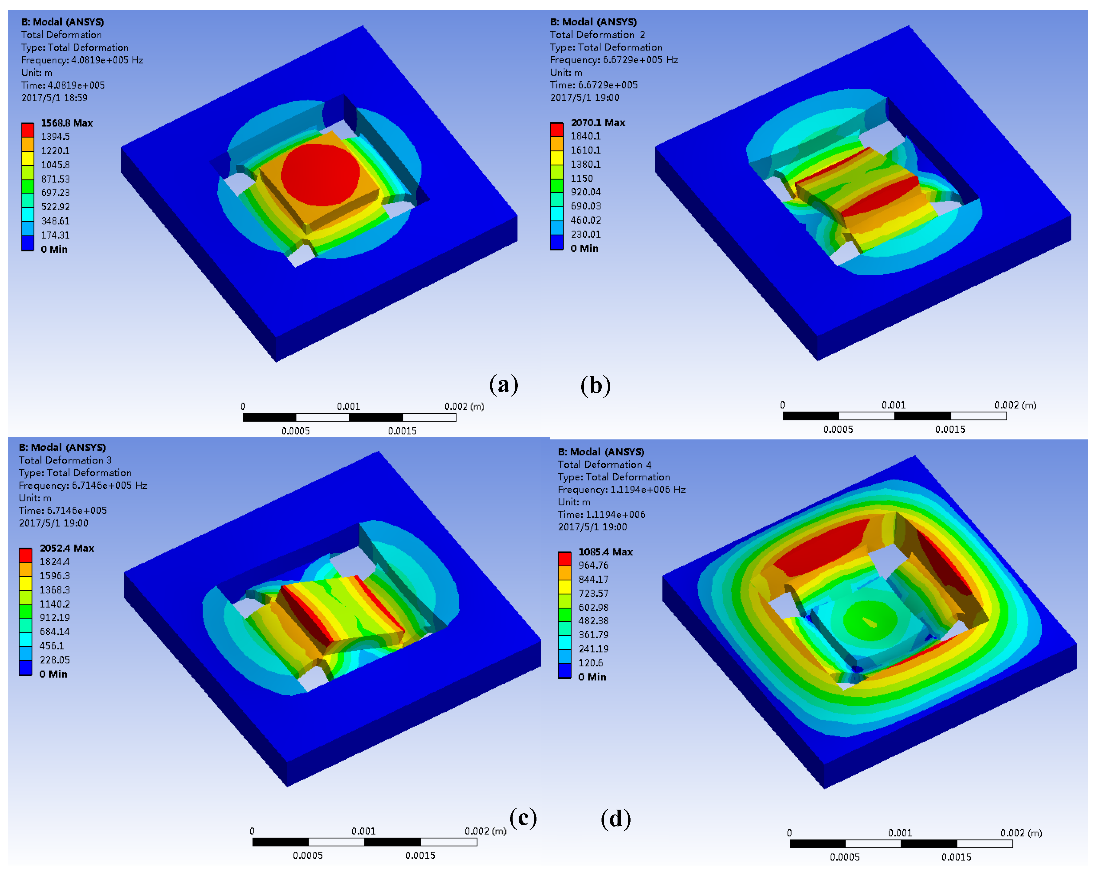
| Mode Shapes | 1 | 2 | 3 | 4 |
|---|---|---|---|---|
| Resonant Frequency (kHz) | 408 | 667 | 671 | 1119 |
| EMD | Wavelet | EMD + Wavelet | Original | ||
|---|---|---|---|---|---|
| Preparing Stage | Bias Stability Value @10−7s (g/h) | 2.9241 × 10⁴ | 3.7970 × 10⁴ | 3.6162 × 10⁴ | 1.0591 × 10⁶ |
| Improves from Original | 97.2% | 96.6% | 96.4% | - | |
| Shock Stage | Value | 2.7712 × 10⁷ | 1.9523 × 10⁷ | 2.8701 × 10⁷ | 2.8702 × 10⁷ |
| Error from Original | 3.49% | 32.1% | 0.003% | - | |
| Vibration Stage | Value | 1.3410 × 10⁵ | 2.2503 × 10⁷ | 4.4251 × 10⁷ | 4.4310 × 10⁷ |
| Error from Original | 99.70% | 49.22% | 0.135% | - |
© 2019 by the authors. Licensee MDPI, Basel, Switzerland. This article is an open access article distributed under the terms and conditions of the Creative Commons Attribution (CC BY) license (http://creativecommons.org/licenses/by/4.0/).
Share and Cite
Lu, Q.; Pang, L.; Huang, H.; Shen, C.; Cao, H.; Shi, Y.; Liu, J. High-G Calibration Denoising Method for High-G MEMS Accelerometer Based on EMD and Wavelet Threshold. Micromachines 2019, 10, 134. https://doi.org/10.3390/mi10020134
Lu Q, Pang L, Huang H, Shen C, Cao H, Shi Y, Liu J. High-G Calibration Denoising Method for High-G MEMS Accelerometer Based on EMD and Wavelet Threshold. Micromachines. 2019; 10(2):134. https://doi.org/10.3390/mi10020134
Chicago/Turabian StyleLu, Qing, Lixin Pang, Haoqian Huang, Chong Shen, Huiliang Cao, Yunbo Shi, and Jun Liu. 2019. "High-G Calibration Denoising Method for High-G MEMS Accelerometer Based on EMD and Wavelet Threshold" Micromachines 10, no. 2: 134. https://doi.org/10.3390/mi10020134
APA StyleLu, Q., Pang, L., Huang, H., Shen, C., Cao, H., Shi, Y., & Liu, J. (2019). High-G Calibration Denoising Method for High-G MEMS Accelerometer Based on EMD and Wavelet Threshold. Micromachines, 10(2), 134. https://doi.org/10.3390/mi10020134